Sage Journals: Discover world-class research

Abstract

Traditional theories of “adolescent risk taking” have not been validated against recent research indicating that youthful traffic crash, violent crime, felony crime, and firearms mortality rates reflect young people’s low-socio-economic status (SES) compared with older adults’, not young age. Aside from a small number of recent, conflicting studies, the literature gap on this key issue remains. The present study examines the 54,094 homicide deaths, including 41,123 gun homicides, victimizing California residents ages 15 to 69 during 1991 to 2012 by poverty status. Without controlling for poverty, homicide rates display the traditional age-curve peaking at 19, then declining. When poverty is controlled, the traditional age-curve persists only for high-poverty populations, in which young people are vastly over-represented, and homicide rates are elevated for all ages. This finding reiterates that “adolescent risk taking” may be an artifact of failing to control for age-divergent SES.

Keywords

adolescents age risk taking homicide guns development

Introduction

Four previous articles have challenged traditional concepts of “adolescent risk taking,” including the “age–crime curve,” for mis-attributing behaviors associated with the high rates of poverty and disadvantage suffered by young people to age-based biological and developmental traits (Brown & Males, 2011; Males, 2009a, 2009b; Males & Brown, 2013b). They argued that traditional theories of natural teenage criminality, violence, recklessness, peer orientation, and risk taking incorporate a traditional error: the failure to control for external disparities in socio-economic status (SES), including conditions of poverty, before imposing concepts of internal bio-developmental limits. The evidence for the claim that “adolescent risk” is an artifact of adolescent poverty is straightforward: Where subjected to the same economic disadvantages, as teenagers are on average, middle-aged adults (thought to be a mature, risk-averse demographic) display higher “teenaged” outcomes with respect to such “adolescent risks” as serious crime, violent crime, firearms mortality, and fatal traffic crashes. Conversely, where teenagers enjoy the same advantaged economic conditions as the average middle-aged adults, teenagers display “middle-aged” outcomes (Brown & Males, 2011; Males & Brown, 2013a, 2013b). These studies do not make any inferences about individual risk taking; their focus is on populations.

Although these studies have proven controversial, the literature disputing their findings is very sparse. Virtually all studies that have advanced traditional assertions of adolescent versus adult risks have failed to control for inter-age disparities in SES; other studies have controlled only for race or geography or examined only a single young cohort. Such limited methods are insufficient to sustain conclusions about adolescent risk taking. Exhaustive literature searches by the authors and by other researchers have revealed only one other study of the interaction of age and economic disadvantage in predicting risk taking: Shulman et al. (2013a), Steinberg, and Piquero’s (2013) analysis of National Longitudinal Survey of Youth (NLSY) data that finds no age–poverty interaction for ages 12 to 23 in self-reported offending. However, this cohort study is limited in age range and fails to control for major confounds such as period effects, as will be discussed.

The absence of adolescent-versus-adult behavior studies that incorporate comparative SES interactions is related to an inconsistency in theoretical treatment. When explaining even large discrepancies in behaviors between population groups, modern theorists and researchers reject internal biological (i.e., neurological) and developmental (i.e., risk taking) traits in favor of external sociological conditions (concentrated poverty, unemployment, discrimination, etc.; Gould, 1981). Researchers and theorists acknowledge the crucial nature of SES disparities when assessing behavior divergences between Adult Population A versus Adult Population B, Adolescent Population A versus Adolescent Population B, and every other comparative analysis—except Adolescent Age A versus Adult Age B. Researchers seem to assume that the effects of SES disparity are inapplicable in only one instance: when youth and adult behaviors are compared.

The failure to analyze divergent adolescent–adult SES as a determining factor in divergent adolescent–adult behavior is compounded by the resurrection of long discredited bio-determinist notions. Recent small-subject functional magnetic resonance imaging (fMRI) studies purportedly showing youths use more primitive areas of the brain than adults in decision-making have been interpreted as biological proof of innate adolescent risk taking, sometimes generating extreme statements. “Adolescents, on average, engage in more reckless behavior than do individuals of other ages” and are “biologically driven” to risk taking, including criminal offending, declared Steinberg (2007, p. 56). Such strident biological interpretations are not warranted at this early stage of brain investigation and involve more prejudice than science, as evidenced by the fact that claims of greater adolescent risk are made even when fMRI findings show adolescents use more sophisticated cortical reasoning than do adults (Baird, Fugelsang, & Bennett, 2005). More recent, decisive reviews of multiple studies have found fMRI findings “puzzlingly” overstated (Vul, Harris, Winkielman, & Pashler, 2009, p. 274) and have failed to replicate earlier fMRI claims (Boekel et al., in press). As brain imagings do not demonstrate greater risk-taking propensity in and of themselves, the theory of adolescent crime proneness remains founded in crime statistics whose age-discrepant external variables have not been controlled prior to assertions of age-discrepant internal drivers.

This study attempts to fill this literature gap by extending the previous analyses of age–poverty interactions to examine one of the most serious forms of alleged “adolescent risk taking”: homicides, especially by firearms. Both research and popular literature regularly depict homicide, especially gun killings, as an adolescent and young adult risk behavior; one prominent team even dubbed these young ages as “deadly demographics” (Fox & Piquero, 2003, p. 339; see also Bennett, DiIulio, & Walters, 1996; National Research Council, 2006; Reyna & Rivers, 2008; Wilson & Herrnstein, 1994). Even the nation’s highest legal authority has depicted homicide as a particular teenaged risk (Supreme Court of the United States, 2012).

Background and Literature Review

Decades of research have consistently upheld that poverty and related social disadvantage are key factors promoting criminality (see Donziger, 1996; Jencks, 1992; Shelden, Tracy, & Brown, 2001), though they disagree as to the extent and mechanisms (Wright, Caspi, Moffitt, & Silva, 1999). The lengthy, general literature reviews in previous studies (see Brown, 2009; Brown & Males, 2011; Males & Brown, 2013a, 2013b) examining varied, historical theories of criminal behavior and reaffirming SES as a critical factor when comparing differences in offending by population groups will not be repeated here. Rather, the present review will extend these past literature reviews by adding the recent, small body of population and cohort studies that examine age and SES in the context of risk behaviors.

There appears little investigation of how poverty interacts with age across the life span to produce theories of deviance and risk taking (Brown & Males, 2011; McCall, Land, Dollar, & Parker, 2012; Phillips, 2006). In particular, there appears no literature other than by Males and Brown that assesses the interaction of poverty, age, and risk behaviors for ages above 24. The sparse literature on age–poverty interactions falls into two categories: population-level studies and cohort studies, each of which present advantages and weaknesses. Cohort studies examine criminal offending longitudinally along a birth cohort as it ages. This vertical approach allows examination of trends within the cohort examined but is vulnerable to “period effects” in that its results are not generalizable to other cohorts that may display different patterns in different time periods. In contrast, population-level studies analyze offending rates horizontally across generations during the same time period, a cross-sectional approach that controls for cohort effects but may not be generalizable to other time periods. It is difficult to apply cohort and population studies to test or refute each other because they use very different assumptions and methods, although synthesizing their findings may prove useful.

Population (Macro-Level) Studies

Study of the effects of personal, socio-economic, and other environmental factors on individual (micro-level) propensities to crime is supplemented by a literature that delineates macro-level (population-wide) influences with strong predictive values on the distribution of crime (Pratt & Cullen, 2005). Both traditional macro-level theories, including institutional anomie and social disorganization (Cancino, Varano, Schafer, & Enriquez, 2007), and more recent analyses (i.e., Sampson, 2012) have documented that community factors powerfully affect criminal behaviors and related social phenomena. One of the most “stable and strongest predictors” of crime is the constellation of factors labeled as “concentrated disadvantage” (Pratt & Cullen, 2005, p. 373), for which poverty rate is a key measure. Individual-level and population-level theories are not mutually exclusive and may be integrated in studies of the mediation of environmental factors on individual behavior (Muftić, 2009).

Three relevant population-level studies by the same authors, Brown and Males (2011) and Males and Brown (2013a, 2013b), use California’s unusually detailed crime statistics to conclude that adolescents’ and young adults’ apparently elevated rates of felony crime, violent crime, and gun violence mortality are due to their low-SES relative to older adults’, not young age. The 2013 article, replicating 2011 results, found that without controlling for SES, crime rates displayed the traditional age–crime curve, peaking in late adolescence and early adulthood (Males & Brown, 2013a). However, when poverty status was controlled by means of comparing crime rates among 906 population cells, each of which represented distinct age, race/ethnicity, county, and poverty values, the traditional age–crime curve largely disappeared. Where middle-aged adults suffered high rates of poverty common to teenagers, they displayed higher “teenage” offending rates; where teenagers enjoyed low middle-aged poverty levels, they displayed lower middle-aged crime rates. That is, “adolescent risk taking” is an artifact of failing to control for age-divergent SES. These studies suggest that adolescents and young adults, like non-White races, suffer higher rates of crime and arrest due to poverty and related economic disadvantages, not demographic characteristics such as age or race.

However, these population-level studies have distinct limitations. Owing to the difficulty of assembling complete, detailed data sets by age, geography, and race and ethnicity over multiple years, these studies examined 1 year’s cross-sections of crime, population, and poverty data for the state of California, a large and diverse geography that may not generalize to other locales. Multi-year data sets would allow for control of cohort effects. Furthermore, population-level studies examine demographic units and are not useful for delineating individual risk.

Cohort Studies

Cohort studies also suffer from data limitations due to the lack of consistent, complete surveys and archival tabulations of representative populations over time. One recent study of an inner-city cohort found that “neighborhoods explain a large percentage of individual-level disparities”; in particular, neighborhoods with high levels of concentrated disadvantage as a result of entrenched poverty are especially criminogenic (Sampson, Morenoff, & Raudenbush, 2005, p. 6). Although “the probability of violence accelerates in early adolescence for all groups [in the study], reaching a peak between the ages of 17 and 18 and then declining precipitously” (Sampson et al., 2005, p. 4), the larger work casts doubt on the theory that aging itself produces a spontaneous desistance from crime. Rather, routine criminal offending diminishes coincident with “turning points” that arise from “opportunities,” such as stable employment, marriage, or wealth accumulation, all of which are confounded with increasing age (Laub & Sampson, 2003). Socio-economic disadvantage appears to intensify and prolong “crime-prone years” from adolescence well into adult ages (Phillips, 2006). Conversely, cities with higher than average proportions of economically and socially engaged young people had lower homicide rates as the proportion of people aged 18 to 29 in their populations increased (Fabio, Tu, Loeber, & Cohen, 2011).

The only cohort study directly assessing the age–poverty interaction appears to be one limited analysis of NLSY respondents born between 1980 and 1984. It found self-reported criminal offending by youths age 12 to 17 (collected in Wave 1 in 1996) declined sharply as that cohort aged into young adults years (collected in Waves 6-7 in 2003), even after economic status was controlled. “The age–crime curve in adolescence and early adulthood is not due to age differences in economic status,” concluded Shulman et al. (2013a, p. 848). Because this study was published explicitly to refute Brown and Males (2011, referred to as the “subject study” in this subsection) and appears the only other study to incorporate SES in addressing the age–crime curve, an extensive analysis of Shulman et al. (2013, referred to as the “counter-study”) is presented here.

First, the counter-study authors’ repeated claims to have “tested” and provided a “strong rebuttal” to Brown and Males (2011) is questionable. A cohort counter-study that uses an “age range . . . restricted to adolescents and young adults” ages 12 to 23 is insufficient to “test” statements in the cross-sectional subject study that encompassed ages 15 to 69. Questions of whether “poverty varies systematically with age,” or that the counter-study’s findings can be combined with previous studies that do not control for SES to argue that biological and developmental reasons explain why “crime is in fact committed disproportionately by the young” (Shulman et al., 2013a, pp. 853, 858) are not supported by the evidence presented.

Second, extensive re-analysis casts strong doubt as to what the counter-study (published 17 years after the baseline year of the cohort it analyzed) actually found. Only some of the major limitations and inconsistencies in the NLSY data base were acknowledged in the counter-study. The acknowledged limitations include the problems that both those providing SES information and the household configurations changed substantially from NLSY Waves 1 (parents) to Waves 6 to 7 (young adults), and that differing proportions in the three waves averaging around one fourth of the total sample provided no SES data. The counter-study’s economic analysis strongly depended on the authors’ assumption that NLSY respondents know “the gross household income (the sum of household members’ wages, child support, investment income, rental income, retirement income, gifts, government support) for the prior year” (Shulman et al., 2013a, p. 852). This might generally be true for parents responding in Wave 1 but is much less likely to be accurate for young adults living with parents or roommates in Waves 6 to 7. How many young adults know all sources of income of their parents or housemates? In fact, parents’ self-reported income status in Wave 1 in 1996 is associated with just .13 to .20 (using the R² values) of the income status reported by young adults in Waves 6 to 7 in 2002 to 2003. The association between income status in Waves 6 to 7, 1 year apart, is just .33; that is, most of those who were poor in 1996, or even in 2002, were not poor in 2003, and vice versa. These are implausibly weak correlations given the unlikeliness of significant income changes within the same (or somewhat the same) set of individuals in such short periods. This indicates the counter-study’s estimates of SES by time period and age are not consistently obtained. Thus, the counter-study cannot be shown to have presented crime rates by earlier (adolescent) and later (young adult) ages standardized to equivalent income statuses over time, a flaw that would negate its conclusions.

The counter-study’s unacknowledged limitations are equally troubling. These include the non-random dropout of 12% to 14% of the sample from NLSY Wave 1 to Waves 6 to 7. As dropouts disproportionately displayed greater personal risk factors than those retained in the survey (Aughinbaugh & Gardecki, 2007), a selection bias is created that may render later waves less likely to commit crime than earlier waves. This bias affects not just self-reports of crime but also the counter-study’s inconsistent measures of income status. These limitations and biases, not uncommon in cohort samples such as NLSY, make this data set difficult to use to analyze age, SES, and offending over time.

Third, and also serious, is the conundrum of “honestly reporting one’s dishonesty,” a validity threat generic to self-reporting surveys (see Lauritsen, 1998). The pattern found in the counter-study could result either from a real decline in offending or from a decline in willingness to report socially disapproved behaviors by age and over time. The suspicion that adults under-report their crime is reinforced by Federal Bureau of Investigation (FBI) clearance reports showing juveniles are over-arrested; that is, they commit a substantially lower proportion of crimes than their arrest proportions would predict. For example, youths under age 18 accounted for 11.1% of violent and 15.7% of property index arrests in 2013, but just 8.8% of violent crimes and 10.8% of property crimes cleared by arrest (FBI, 2014). Lotke (1997) found that fewer than half the youths arrested for homicide were ultimately charged with that offense. The American Civil Liberties Union (ACLU; 2013) study of 13,000 Oakland juvenile arrests found 56.6% were not sustained; while these showed up on official tabulations of arrests, probation officers found no criminal activity meriting further action.

Similarly, public health statistics tied to a variety of crimes, such as hospital emergency treatments and deaths from abusing illicit drugs, peak at ages well beyond teen years. Taken together, independent measures indicate that the self-report data the counter-study relies on is not convergent with official records. The authors’ failure to present strong literature findings of consistent self-reporting of offending across the life span is a critical omission. While the subject study uses a data set (arrests) that is biased against its hypothesis that youth and adult crime rates equalize once SES is controlled, the counter-study’s data set (self-reported offending) appears biased in favor of its hypothesis that adolescents commit more crime than do adults.

Finally, due to admitted limitations and inconsistencies in the NLSY, the counter-study by necessity used an out-of-date cohort that fails to capture major changes in youth and adult offending patterns—including dramatic weakening of the age–crime curve—in recent decades that have been particularly pronounced in the last 15 years (FBI, 2014). Criminal arrest rates, particularly by younger ages, declined sharply from 1996 through 2003—the time period used in the counter-study—and continued declining through 2013, the most recent year available (Figure 1). In 1996, arrest rates peaked at age 18 and displayed the familiar age–crime curve. After a substantial decline in teenage crime rates and a lesser decline in 20-age crime by 2003, arrest rates then peaked at age 19 and the age–crime curve had weakened considerably. After even larger declines in crime among teenagers through 2013, arrest rates peaked at age 21, and the age–crime curve all but disappeared. Self-reported and victim-reported offending measures also show disproportionate declines in youthful offending from 1996 to 2003 and thereafter (Males & Brown, 2013a). The overall crime decline concentrated in young ages easily accounts for the lower rate of self-reported offending by ages 19 to 23 in Waves 6 to 7 in 2003 compared with ages 12 to 17 in Wave 1 in 1996 independently of any effects from aging. The failure of the counter-study to include a control series (which is not available in the NLSY) to adjust for general changes in crime also risks negating its findings.

Figure 1.

Youth offending as a period effect declined sharply from 1996 (corresponding to NLSY, Wave 1) to 2003 (corresponding to NLSY, Waves 6-7), and through 2013.

Authors further make no effort to control for “college poverty,” the temporarily low incomes of college students who typically also have low crime rates, a major problem given the counter-study’s limited, under-24 age range and inconsistent income measure. The “college poverty” issue was acknowledged in the subject study but constituted less of a problem because of that study’s much broader age range.

In every case, the critical limitations and omissions of the counter-study contribute to a pro-hypothesis bias. The advantage of the NLSY’s potential to capture offenses not reported to police is more than offset by its limitations in terms of confinement to a single, outdated, young cohort age, inconsistent measurement of SES and offending, and attrition of higher-risk subjects over time. Regression models by race and economic status derived from the counter-study’s single, limited, and confounded data set cannot reliably demonstrate a generalizable age–crime curve even within their truncated age range, let alone serve as a challenge to newer, population-level studies encompassing much broader age ranges. Age, SES, and offending clearly require more analysis.

Method

The present study uses population-level analysis of two crime predictors: age and poverty rate. The premise derived empirically from macro-level statistics is that young populations differ substantially from older populations in more ways—and potentially more important ways—than just age. One barrier to analysis is that SES variables such as poverty level are not captured in the official arrest statistics typically used to construct crude age–crime curves. An alternative measure, self-reporting surveys of criminal behavior, enables tabulations of individual socio-economic variables that are not captured in official crime statistics, but self-reports may be incomplete and unreliable (Lauritsen, 1998), and, in particular, may vary in reliability with age as previously discussed.

A third alternative, used here, is to use risk outcome and census statistics to conduct population-level investigations into whether disproportionately low-SES and high concentration of high-arrest demographics among young people, as opposed to young age per se, explains the “age–homicide curve” in the same way they would explain the “race–homicide curve.” Homicide, particularly firearms homicide, fatality has been extensively cited as exemplifying the most serious kind of age-based risk.

Homicide Tabulations

As an index, homicide has distinct advantages and disadvantages. It is subject to rigorous investigation and is the only criminal offense also tabulated as a vital statistics event. In California, homicide deaths are available from the state’s Center for Health Statistics’ EPICenter (2014) for the 1991 to 2012 period in considerable detail, providing homicide method and single year of age by race and Hispanic ethnicity by county of residence. This 22-year study period includes years of both high- and low-homicide tolls and thus minimizes both period and cohort effects as well as selection biases. However, it is a relatively rare offense requiring large populations and multiple years to show definitive, detailed patterns.

To minimize the crime-inhibiting physical limitations of very young and very old age, only ages 15 to 69 are assessed. For these ages, all homicide deaths (N = 54,094), gun homicide deaths (n = 41,123), and non-gun homicide deaths (n = 12,977) are tabulated for the four major races (Hispanic, White not Hispanic, Black not Hispanic, Asian/Other not Hispanic), for eleven 5-year age groups (15-19 through 65-69), and for the state’s 58 counties for the study period. These tabulations produced 2,552 raw, age-by-race-by-county cells statewide.

Populations and Poverty Rates

Populations by single year of age, race and Hispanic ethnicity, county of residence, and year are available from EPICenter (2014) and the California Department of Finance (2014) for the entire period. Poverty rates—the percentage of the population living in households with incomes below federal poverty guidelines—by age group, race, and county for 1999, a central year in the study period, are available from the Bureau of the Census (2014) for 88% of these 2,552 cells. After excluding the 305 minimal population cells without calculated poverty rates, 2,247 cells containing 99.95% of the state’s population remained available for analysis. Poverty rates by single years of age by race and county were imputed from grouped-age poverty rates by standard linear interpolation (Shyrock & Siegel, 1976).

Analysis

For ages 15 to 69, separate homicide counts, population counts, homicides per 100,000 population, and percentage of the population in poverty were calculated separately for each race, 5-year age group, 5% poverty bracket, and county by standard SPSS software. Age groups were further collapsed into standard 5-year age groups for those under age 30 and 10-year age groups for those 30 and older. Due to very small numbers of young people in the two lowest poverty brackets and very few older ages in the two highest poverty brackets, the lowest and highest poverty rates were combined into less than 10% and more than 25% brackets (Table 1). This analysis is repeated for firearms homicides and non-gun homicides. Excel charting functions produced both the crude point-to-point arithmetic trendlines and the polynomial regression lines based on least-squares expressions incorporating all data points into a continuous curve, shown in Figures 2 and 3.

Table 1.

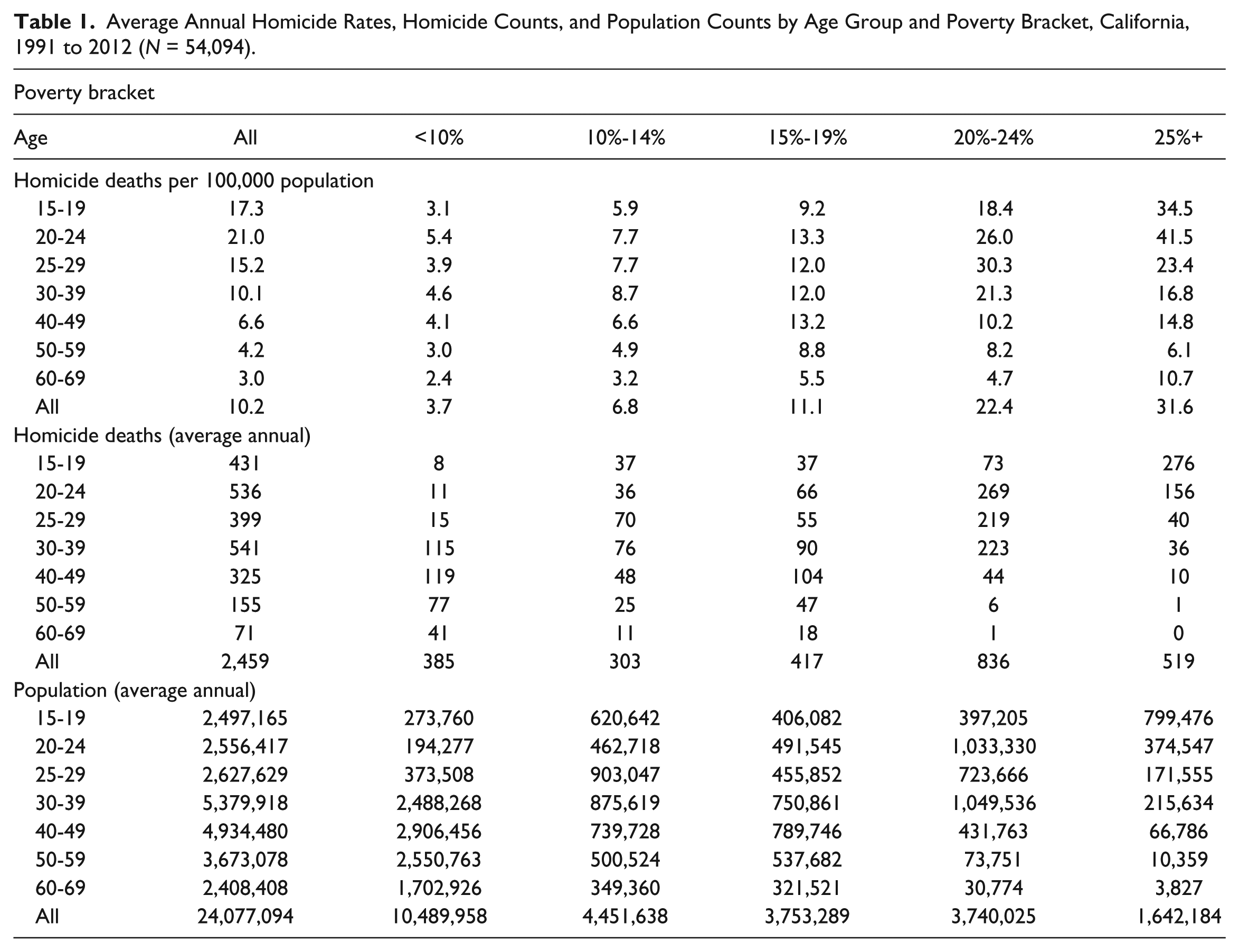
Average Annual Homicide Rates, Homicide Counts, and Population Counts by Age Group and Poverty Bracket, California, 1991 to 2012 (N = 54,094).

Poverty bracket
Age	All	<10%	10%-14%	15%-19%	20%-24%	25%+
Homicide deaths per 100,000 population
15-19	17.3	3.1	5.9	9.2	18.4	34.5
20-24	21.0	5.4	7.7	13.3	26.0	41.5
25-29	15.2	3.9	7.7	12.0	30.3	23.4
30-39	10.1	4.6	8.7	12.0	21.3	16.8
40-49	6.6	4.1	6.6	13.2	10.2	14.8
50-59	4.2	3.0	4.9	8.8	8.2	6.1
60-69	3.0	2.4	3.2	5.5	4.7	10.7
All	10.2	3.7	6.8	11.1	22.4	31.6
Homicide deaths (average annual)
15-19	431	8	37	37	73	276
20-24	536	11	36	66	269	156
25-29	399	15	70	55	219	40
30-39	541	115	76	90	223	36
40-49	325	119	48	104	44	10
50-59	155	77	25	47	6	1
60-69	71	41	11	18	1	0
All	2,459	385	303	417	836	519
Population (average annual)
15-19	2,497,165	273,760	620,642	406,082	397,205	799,476
20-24	2,556,417	194,277	462,718	491,545	1,033,330	374,547
25-29	2,627,629	373,508	903,047	455,852	723,666	171,555
30-39	5,379,918	2,488,268	875,619	750,861	1,049,536	215,634
40-49	4,934,480	2,906,456	739,728	789,746	431,763	66,786
50-59	3,673,078	2,550,763	500,524	537,682	73,751	10,359
60-69	2,408,408	1,702,926	349,360	321,521	30,774	3,827
All	24,077,094	10,489,958	4,451,638	3,753,289	3,740,025	1,642,184

Figure 2.

Unadjusted gun, non-gun, and total homicide rates per 100,000 population by age, with polynomial trendlines, California, 1991 to 2006.

Figure 3.

Age–homicide rate curve by age group at six standard poverty brackets, with crude (light dashed) and polynomial regression (solid) trendlines, California, 1991 to 2012.

Results

Age and Poverty Levels

Table 1 provides the sums of homicide counts and populations by age group and poverty bracket. Poverty is heavily concentrated in younger ages. California’s teenagers and young adults occupy very different economic environments on average than older adults. More than half (52%) of 15- to 24-year-olds are in population cells with poverty levels averaging 20% or higher, compared with fewer than 7% of adults in their 40s and 50s. Conversely, just 9% of 15- to 24-year-olds occupy cells with poverty rates averaging below 10%, compared with over 63% of 40- to 59-year-olds. Even within 5% or 10% poverty brackets, younger people’s average poverty rate is higher than for older ages.

Commensurate with higher poverty levels, youths and young adult populations have substantially higher proportions of African and Hispanic Americans, whose homicide death and arrest rates generally are higher than for Whites and Asians, than do older ages. In California over the study period, 50% of ages 15 to 19 are Black or Latino, compared with 30% for ages 40 to 69.

Age and Homicides

For all ages, homicides are disproportionately concentrated in the poorest brackets, but the impact is much more pronounced for younger ages (Table 2). Among 15- to 24-year-olds, 81% of homicides (including 83% of gun and 65% of non-gun homicides) occurred among the occupants of brackets with poverty levels of 20% or higher, while fewer than 2% of homicides (including 1.4% of gun homicides and 4.5% of non-gun homicides) occurred among the occupants of poverty brackets below 10%. Older ages also show much higher rates of homicide among those in the 20+% poverty brackets compared with those in poverty brackets below 10%, but there are so few occupants age 40 and older in the highest poverty categories that homicide rates are more erratic and the overall impact of poverty is much lower.

Table 2.

Average Annual Gun and Non-Gun Homicide Rates and Counts by Age Group and Poverty Bracket, California, 1991 to 2012 (n = 41,123 for Gun, n = 12,971 for Non-Gun).

Poverty bracket
Age	All	<10%	10%-14%	15%-19%	20%-24%	25%+
Gun homicide deaths per 100,000 population (average annual)
15-19	15.3	1.8	4.5	7.5	16.2	31.8
20-24	17.8	3.7	5.5	10.5	22.4	37.1
25-29	12.3	2.4	5.6	9.2	26.2	19.2
30-39	7.4	2.9	6.3	8.7	17.0	11.7
40-49	4.0	2.2	4.0	8.9	6.8	8.7
50-59	2.2	1.4	2.5	5.2	4.2	3.5
60-69	1.4	1.0	1.6	3.0	1.9	5.9
All	7.8	2.0	4.7	7.9	18.6	27.9
Non-gun homicide deaths per 100,000 population (annual average)
15-19	2.0	1.3	1.5	1.8	2.2	2.7
20-24	3.2	1.7	2.2	2.9	3.6	4.4
25-29	2.8	1.5	2.1	2.8	4.1	4.2
30-39	2.7	1.7	2.4	3.3	4.3	5.1
40-49	2.6	1.9	2.5	4.3	3.4	6.1
50-59	2.0	1.6	2.4	3.6	4.0	2.6
60-69	1.6	1.4	1.5	2.5	2.8	4.8
All	2.4	1.7	2.1	3.2	3.7	3.7
Gun homicide deaths (annual average)
15-19	381	5	28	30	64	254
20-24	455	7	26	51	231	139
25-29	324	9	51	42	189	33
30-39	396	72	55	65	178	25
40-49	199	64	30	70	29	6
50-59	81	36	13	28	3	0
60-69	34	18	6	10	1	0
All	1,869	212	207	297	696	458
Non-gun homicide deaths (annual average)
15-19	50	3	9	7	9	22
20-24	82	3	10	14	38	17
25-29	74	6	19	13	30	7
30-39	145	43	21	25	45	11
40-49	126	54	19	34	15	4
50-59	75	40	12	19	3	0
60-69	38	23	5	8	1	0
All	590	173	96	120	140	61

Age, Poverty, and Gun Homicide Rates

Crude rates of gun homicide mortality by age group, unadjusted for poverty level—that is, the familiar age–murder curves, including their polynomial distributions—are shown in Figure 2. In the unadjusted distribution, both homicide and gun homicide rates peak at age 19 and decline thereafter, and rates for age 15 to 19 are 3 to 4 times higher than for ages 40 to 49.

Table 1 and Figure 3 show the complex results for homicide rates when poverty rates are held constant across age groups. When poverty levels are held constant, the traditional age–risk curve, with rates peaking in teenage and young adult years and declining thereafter, shows up only for poverty levels of 20% or higher. These high-poverty brackets containing just half the teenage and young adult populations but accounting for four fifths of teenage and young adult gun homicides are the ones that generate crude, unadjusted age–homicide curves.

At poverty levels below 20%, age–risk curves are weak and ambiguous, and teenaged rates become unremarkable. A delayed age–crime curve appears at a constant poverty level of 15% to 19%, with homicide rates peaking in the 20s and 30s and age 15-to-19’s rates similar to those of adults in their late 30s. In the 10% to 14% poverty bracket, the peak occurs after age 30, and 15- to 19-year-olds’ rates are similar to those in their 40s and 50s. At poverty levels below 5%, only an average of 0.2 gun homicides per year occurred among the small population (2,500) aged 15 to 24 in that bracket, producing rates that were low and erratic.

The goodness-of-fit of the polynomial trendlines to the arithmetic trendlines is strong for poverty levels of 5% or higher, with R² values of well over .90 for poverty levels of 10% or higher, .82 for 5% to 9% poverty levels, and .54 for the smaller, more erratic numbers at poverty levels of 0% to 4%, all of which are strongly significant. The near-complete absence of young people from low poverty and older ages from high-poverty brackets renders gun homicide rates more erratic and error terms larger, but the association of poverty with more homicide remains.

Discussion

Two salient facts, the first well accepted among modern researchers and the second well documented by standard social indexes, are evident: (a) poverty and social disadvantage are crucial variables in assessing comparative levels of criminal offending and other risks among varied populations, and (b) adolescents, young adults, and older adult populations differ in significant ways other than just age, including poverty level and other measures of disadvantage. This study represents the latest validation of a long line of social science research that incorporates measures of disadvantage as standard controls when evaluating statistical variations among population groups—but which, curiously, have only rarely and recently been applied to comparative studies of risk by age.

In every case we have investigated of supposedly signature “adolescent risks”—fatal traffic crashes, firearms mortality, felony crime, violent crime, and, in the present study, homicide and firearms homicide—we find they are severely mitigated or disappear altogether once the economic playing field is leveled. The “age–crime curve” does exist in two ways: (a) at every poverty level, murder rates drop off in the 50s and 60s, and (b) at poverty levels of 20% or higher, the traditional age–crime curve prevails. It is the very high gun homicide level (and to a much lesser extent, the higher non-gun homicide level) in the poorest brackets occupied heavily by young people that create the traditional “age–risk” curve. That is, adolescent risks are artifacts of the reality that the overwhelming majority of serious adolescent crimes, including homicide, and other risk outcomes are concentrated in the poorest demographics—those with poverty rates of 20% to 25% and higher—in which middle-aged and older adults are seldom found.

Under this revised theory, young people do not “age out” of crime, they “wealth out.” The failure to consider SES as a determinant in offending may also explain why studies attempting to forecast crime trends from the age structure of the population have proven so quickly and notoriously inaccurate (Levitt, 1999; Males & Brown, 2013b).

Because poverty is an acknowledged, crucial variable and the young are much poorer than the old, research that purports to affirm adolescent risk taking while failing to incorporate measures of age-based disadvantage in comparing risks across the life span represents a deviation from standard social science practice. Unfortunately, some researchers propose to perpetuate this omission. Shulman et al. (2013a; 2013b) summarized new efforts by “developmental scientists from diverse backgrounds” who “have been making rapid progress toward an integrated theory” that would explain “at multiple levels” why “there is something about adolescence as a developmental period that inclines youth toward law-breaking behavior” and “increased willingness to engage in risky conduct” (pp. 848, 858-859). Concluding that their single, age-limited, methodologically flawed, and fatally confounded study of one young NLSY cohort has effectively established that “the age–crime curve in adolescence and early adulthood is not due to age differences in economic status,” they welcome an “integrated theory” that

incorporates findings from neuroscientific work investigating structural and functional changes in the brain that take place during adolescence and may facilitate risk-seeking, as well as results from psychological research examining age-related changes in traits (e.g., sensation-seeking, reward salience, and susceptibility to peer influence) related to this type of behavior. (Shulman et al., 2013a, pp. 858-859)

Yet, developmentally and neurologically based risk concepts remain poorly grounded. That “something about adolescence,” as we have shown in several studies, is a poverty level 2 to 3 times higher than among middle-aged adults—a “something” that middle-aged adults, when subjected to it at teenaged levels, is also associated with middle-agers’ greatly heightened rates of crime and other risks. Economic disadvantage is the same “something about African Americans,” “something about Native Americans,” and “something about Mississippians” that is associated with statistical excesses for many risks—a “race–crime curve” or a “geography–crime curve”—in these groups. However, this is not to say that higher poverty, greater disadvantage, and lower SES engender the same effects within populations, and certainly do not produce the same effects among individuals. With regard to age, Joseph Adelson (2008) points out, “transitional periods—from early childhood to middle age”—produce their own types of “inner and outer discord,” and many individuals will not display tendencies found among other of their age-mates (p. 157).

For example, the fact that rates of a comprehensive risk index, violent death (accident, suicide, homicide, and undetermined deaths), are substantially higher among supposedly risk-averse Americans ages 48 to 54 (75.5 per 100,000 population in 2012)—including surprisingly high risks among non-Hispanic Whites (84.8)—than among the supposedly risk-prone, more racially diverse ages 18 to 24 (60.1; Centers for Disease Control and Prevention [CDC], 2014), could be used to formulate an integrated, bio-developmental theory of innate middle-aged cognitive deterioration (see Azar, 2010; Lu et al., 2004; Schaie & Willis, 2008) and risk taking. Yet, excessive and rising external mortality, along with rising criminal arrest (FBI, 2014), among American middle-agers (despite their generally high-SES and low-poverty levels) has received virtually no scholarly or policy attention. If it did, one can safely bet the focus would be on external conditions, not internal biologies. Investigations consistently suggest that adults, including researchers, favor their own aging peers while subscribing to systematically negative stereotypes toward adolescents (see Adelson, 2008; Buchanan et al., 1990; Enright, Levy, Harris, & Lapsley, 1987; Hill & Fortenberry, 1992; Offer, Ostrov, & Howard, 1981; Offer & Schonert-Reichl, 1992; Public Agenda, 1999; Quadrel, Fischhoff, & Davis, 1993) that constitute “a stubborn, fixed set of falsehoods,” as Adelson (1979, p. 33) termed it 35 years ago and recently reaffirmed. In a review of 150 studies, Offer and Schonert-Reichl (1992) lamented that so many, including researchers, “continue to believe many of the myths about adolescence” (p. 1004).

In that light, the “integrated theory” purporting to merge biological- and developmental-stage theories to speculate why adolescents “act the way they do” (Shulman et al., 2013a) is simply the latest resurrection of 19th century notions that combined supposedly innate biological- and phylogenic-stage notions into theories speculating why races, ethnicities, and genders “acted the way they did” (see Gould, 1981). One only need consider the fact that homicide rates are 18 times higher among the poorest than the wealthiest teenagers—or that 51,000 California 15- to 19-year-olds in the lowest poverty brackets experience an average of just 1.1 murders per year (a European level), or that 40-agers and 50-agers subjected to the same poverty levels as older teenagers display the same levels of homicide (see Table 1)—to come to the conclusion that innate biological and developmental imperatives are at best marginal drivers of late adolescent and young adult offending.

Limitations

This study continues preliminary, population-level investigation of risk outcomes by age. It concerns the association of risk with environments of poverty and, to avoid the “ecological fallacy,” cannot be used to predict individual outcomes. The study is confined to homicide and gun homicide, rare but well defined and comprehensively tabulated outcomes that have been asserted to display the traditional “age-crime” pattern, and may not apply to unstudied risks. It is confined to California, a populous state with large representations of varied demographics that, nevertheless, may not be generalizable to other geographies.

Footnotes

Acknowledgements

Elizabeth Brown, professor of Criminal Justice Studies, San Francisco State University, assisted in the literature review.

Declaration of Conflicting Interests

The author(s) declared no potential conflicts of interest with respect to the research, authorship, and/or publication of this article.

Funding

The author(s) received no financial support for the research and/or authorship of this article.

Author Biography

Mike Males, PhD, is a senior research fellow at the Center on Juvenile and Criminal Justice, San Francisco, and formerly taught sociology at the University of California, Santa Cruz. He has authored four books and dozens of journal articles on youth issues.

References

Adelson

(1979, February). Adolescents and the generalization gap. Psychology Today, 12, 33-37.

Adelson

(2008). Inventing adolescence. New Brunswick, NJ: Transaction.

Aughinbaugh

Gardecki

R. M.

(2007). Attrition in the National Longitudinal Survey of Youth 1997. Washington, DC: Bureau of Labor Statistics.

Azar

(2010). Your brain on culture. Science Watch, 41(10), 44.

Baird

Fugelsang

Bennett

(2005, April). “What were you thinking?” An fMRI study of adolescent decision making. Poster presented at the 12th Annual Cognitive Neuroscience Society (CNS) Meeting, New York, NY.

Bennett

DiIulio

J. J.

Jr. Walters

(1996). Body count. New York, NY: Simon & Schuster.

Boekel

Wagenmakers

E.-J.

Belay

Verhagen

A. J.

Brown

S. D.

Forstmann

B. U.

(2013). A purely confirmatory replication study of structural brain-behavior correlations. Journal of Neuroscience, 12, 4745-4765.

Brown

(2009). Race, space and crime: Moral panic, the city and “risky” youth. In Krinsky

(Ed.), Children and moral panics. London, England: Ashgate.

Brown

Males

(2011). Does age or poverty level best predict criminal arrest and homicide rates? A preliminary investigation. Justice Policy Journal, 8(1), 1-30. Retrieved from http://www.cjcj.org/uploads/cjcj/documents/Does_age.pdf

10.

Buchanan

C. M.

Eccles

J. S.

Flanagan

Midgley

Feldlaufer

Harold

R. D.

(1990). Parents’ and teachers’ beliefs about adolescents: Effects of sex and experience. Journal of Youth and Adolescence, 19, 363-394.

11.

Bureau of the Census. (2014). American Factfinder: Decennial Census data, American Community Survey data, 2010. Retrieved from http://factfinder2.census.gov/faces/nav/jsf/pages/index.xhtml

12.

California Department of Finance. (2014). Demographic research. Retrieved from http://www.dof.ca.gov/research/demographic/

13.

Cancino

J. M.

Varano

S. P.

Schafer

J. A.

Enriquez

(2007). An ecological assessment of property and violent crime rates across a Latino urban landscape: The role of social disorganization and institutional anomie theory. Western Criminology Review, 8(1), 69-87.

14.

Centers for Disease Control and Prevention. (2014). Injury Prevention and Control. WISQARS, fatal injury data. Atlanta, GA. Retrieved from http://www.cdc.gov/injury/wisqars/fatal_injury_reports.html

15.

Donziger

(Ed.). (1996). The real war on crime: The report of the National Criminal Justice Commission. New York, NY: HarperCollins.

16.

Enright

R. D.

Levy

V. M.

Harris

Lapsley

D. K.

(1987). Do economic conditions influence how theorists view adolescents? Journal of Youth and Adolescence, 16, 541-549.

17.

EPICenter. (2014). Overall injury surveillance. California Department of Public Health. Retrieved from http://epicenter.cdph.ca.gov/ReportMenus/CustomTables.aspx

18.

Fabio

Loeber

Cohen

(2011). Neighborhood socioeconomic disadvantage and the shape of the age–crime curve. American Journal of Public Health, 101, S325-S332.

19.

Federal Bureau of Investigation. (2014). Crime in the United States, 2013, and previous annual reports. Washington, DC: U.S. Department of Justice. Retrieved from http://www.fbi.gov/about-us/cjis/ucr/crime-in-the-u.s/2010/crime-in-the-u.s.-2010

20.

Fox

J. A.

Piquero

(2003). Deadly demographics: Population characteristics and forecasting homicide trends. Crime & Delinquency, 49, 339-359.

21.

Gould

S. J.

(1981). The mismeasure of man. New York, NY: Norton.

22.

Hill

R. F.

Fortenberry

J. D.

(1992). Adolescence as a culture-bound syndrome. Social Science & Medicine, 35, 73-80.

23.

Jencks

(1992). Rethinking social policy: Race, poverty, and the underclass. Cambridge, MA: Harvard University Press.

24.

Laub

J. H.

Sampson

R. J.

(2003). Shared beginnings, divergent lives: Delinquent boys to age 70. Cambridge, MA: Harvard University Press.

25.

Lauritsen

J. L.

(1998). The age-crime debate: Assessing the limits of longitudinal self-report data. Social Forces, 77(1), 127-154.

26.

Levitt

(1999). The limited role of changing age structure in explaining aggregate crime rates. Criminology, 37, 581-597.

27.

Lotke

E. R.

(1997). Youth homicide: Keeping perspective on how many children kill. Valparaiso University Law Review, 31, 395-418.

28.

Pan

Kao

Kohane

Chan

Yankner

(2004). Gene regulation and DNA damage in the ageing human brain. Nature, 429, 883-891.

29.

Males

(2009a). Does the adolescent brain make risk-taking “inevitable?” A skeptical appraisal. Journal of Adolescent Research, 24(1), 3-20.

30.

Males

(2009b). Poverty as a determinant of young drivers’ fatal crash risks. Journal of Safety Research, 40, 443-448.

31.

Males

Brown

(2013a). Authors’ rejoinder to respondents (Shulman et al. (2013b), Steinberg, & Piquero, 2013). Journal of Adolescent Research, 29, 35-44. doi:10.1177/0743558413508204

32.

Males

Brown

(2013b). Teenagers’ high arrest rates: Features of young age or youth poverty? Journal of Adolescent Research, 29, 3-24. doi:10.1177/0743558413493004

33.

McCall

P. L.

Land

K. C.

Dollar

C. B.

Parker

K. F.

(2012). The age structure-crime rate relationship: Solving a long-standing puzzle. Journal of Quantitative Criminology, 29, 167-190. doi:10.1007/s10940-012-9175-9

34.

Muftić

L. R.

(2009). Macro-micro theoretical integration: An unexplored theoretical frontier. Journal of Theoretical and Philosophical Criminology, 1(2), 33-71.

35.

National Research Council. (2006). A study of interactions: Emerging issues in the science of adolescence workshop summary. Washington, DC: Program Committee for a Workshop on the Synthesis of Research on Adolescent Health and Development.

36.

Offer

Ostrov

Howard

K. I.

(1981). The mental health professional’s concept of the normal adolescent. AMA Archives of General Psychiatry, 38(1), 149-153.

37.

Offer

Schonert-Reichl

(1992). Debunking the myths of adolescence: Findings from recent research. Journal of the American Academy of Child & Adolescent Psychiatry, 31, 1003-1014.

38.

Phillips

J. A.

(2006). The relationship between age structure and homicide rates in the United States, 1970 to 1999. Journal of Research on Crime & Delinquency, 43, 230-260.

39.

Pratt

T. C.

Cullen

F. T.

(2005). Assessing the macro-level predictors and theories of crime: A meta-analysis. Crime and Justice, 32, 373-450.

40.

Public Agenda. (1999). Kids these days (Public Agenda resources). Retrieved from http://www.publicagenda.org/media/kids-these-days-99

41.

Quadrel

M. J.

Fischhoff

Davis

(1993). Adolescent (in)vulnerability. American Psychologist, 48, 102-116.

42.

Reyna

Rivers

(2008). Current directions in risk and decision making [Special issue]. Developmental Review, 28(1), 1-152.

43.

Sampson

R. J.

(2012). Great American city: Chicago and the enduring neighborhood effect. Chicago, IL: University of Chicago Press.

44.

Sampson

R. J.

Morenoff

J. D.

Raudenbush

(2005). Social anatomy of racial and ethnic disparities in violence. American Journal of Public Health, 95, 224-232.

45.

Schaie

K. W.

Willis

S. L.

(2008). The Seattle Longitudinal Study. Department of Psychiatry and Behavioral Sciences, University of Washington. Retrieved from http://geron.psu.edu/sls/researchers/index.htm

46.

Shelden

R. G.

Tracy

S. K.

Brown

W. B.

(2001). Youth gangs in American society (2nd ed.). Belmont, CA: Wadsworth.

47.

Shulman

E. P.

Steinberg

Piquero

A. R.

(2013a). The age–crime curve in adolescence and early adulthood is not due to age differences in economic status. Journal of Youth and Adolescence, 42, 848-860.

48.

Shulman

E. P.

Steinberg

Piquero

A. R.

(2013b). A mistaken account of the age–crime curve: Response to Males and Brown (2013). Journal of Adolescent Research, 29, 25-34. doi:10.1177/0743558413493005

49.

Shyrock

H. S.

Siegel

(1976). The methods and materials of demography. San Diego, CA: Academic Press.

50.

Steinberg

(2007). Risk taking in adolescence: New perspectives from brain and behavioral science. Current Directions in Psychological Science, 16(2), 55-59.

51.

Supreme Court of the United States. (2012). Miller v. Alabama (No. 10–9646, Certiorari to the Court of Criminal Appeals, Alabama), Jackson v. Hobbs (No. 10–9647, Certiorari to the Supreme Court of Arkansas). Decided June 25, 2012.

52.

Vul

Harris

Winkielman

Pashler

(2009). Puzzlingly high correlations in fMRI studies of emotion, personality, and social cognition. Perspectives on Psychological Science, 4, 274-290.

53.

Wilson

J. Q.

Herrnstein

(1994). What to do about crime. Commentary, 98(2), 25-33.

54.

Wright

B. R. E.

Caspi

Moffitt

T. E.

Silva

P. A.

(1999). Reconsidering the relationship between SES and delinquency: Causation but not correlation. Criminology, 37(1), 175-194.

Age,Poverty,Homicide,and Gun Homicide

Abstract

Keywords

Introduction

Background and Literature Review

Population (Macro-Level) Studies

Cohort Studies

Method

Homicide Tabulations

Populations and Poverty Rates

Analysis

Results

Age and Poverty Levels

Age and Homicides

Age, Poverty, and Gun Homicide Rates

Discussion

Limitations

Footnotes

Acknowledgements

Declaration of Conflicting Interests

Funding

Author Biography

References