Sage Journals: Discover world-class research

Abstract

Current Generally Accepted Accounting Principles (GAAP) state that the cost of an asset acquired for cash is the fair value (FV) of the amount surrendered, and that of an asset acquired in a non-monetary exchange is the FV of the asset surrendered or, if it is more “clearly evident,” the FV of the acquired asset. The measurement method prescribed for a non-monetary exchange ignores valuable information about the “less clearly evident” asset. Thus, we suggest that the FV in any exchange be measured by the weighted average of the exchanged assets’ FV estimations, where the weights are the inverse of the variances’ estimations. This alternative valuation process accounts for the uncertainty involved in estimating the FV of each of the asset in the exchange. The proposed method suits all types of exchanges: monetary and non-monetary. In a monetary transaction, the weighted average equals the cash paid because the variance of its FV is nil.

Keywords

barter cost entry price exit price fair value non-monetary assets exchange

Introduction

The Accounting Principles Board (APB) in its Opinion 29: Accounting for Non-monetary Transactions, which The Financial Accounting Standards Board (FASB) adopted, sets forth the accounting treatment for a non-monetary exchange (APB, 1973). Three principles constitute the core of Opinion 29: (a) The fair value (FV) of an exchanged asset is the basis for measuring and recording cost; (b) the FV of the surrendered asset is, in general, the cost of the acquired asset; and (c) the FV of the acquired asset may serve as cost when it is “more clearly evident” than that of the surrendered asset. The International Accounting Standards Board (IASB; 1993a, 1993b, 1993c) adopted similar principles.

In line with the current accounting standard, if the FV of both assets exchanged are “clearly evident” to the same extent, and one asset has a FV estimation of $100 and the other asset has a FV estimation of $110, then each party to the exchange will record different amount. However, if the exchange does not involve equalizing cash payment, the FV of both assets must be identical. We, therefore, suggest a procedure to estimate the FV of the exchange by the weighted average of the two assets’ FV estimations, where the weights are the inverse of the variances’ estimations. This alternative valuation process accounts for the uncertainty involved in estimating the FV of each of the assets involved in the exchange. The suggested method unifies the accounting for all types of exchanges (monetary and non-monetary) as it can be implemented to any type of exchange. For example, if one of the assets involved is cash (e.g., buying a machine for $100 in cash) the weighted average is equal to the amount of cash, as the variance of the FV of cash is 0.

Our alternative enables both parties to record the transaction at a single amount, a quality that might be required by tax authorities. We may generalize the model to fit any type of exchange: assets for assets or services, liabilities for assets or services, equity instruments for assets, liabilities, or services, and so forth. Currently, the accounting profession refers to each type of an exchange as a unique case. For example, SFAS 123R (FASB, 2004) establishes standards for transactions in which an entity exchanges its equity instruments for goods or services. Adoption of the proposed model as a general accounting standard will result in one accounting rule for estimating FVs in any type of exchange.

The article contributes to the accounting body of knowledge in the following ways: (a) It offers a general standard for estimating cost for all exchange transactions (monetary and non-monetary); (b) it points out the deficiencies of the current standard for measuring cost in a non-monetary barter; (c) it reveals a number of inconsistencies between accounting standards.

The organization of the article is as follows. The next section provides a short background. The “Models for Analysis” section presents the three models. It discusses their rationale, presents their basic elements, and provides formal results. The final section details the contribution and summarizes the article.

Background

Asset valuation has been a central issue in accounting for quite a long period because of its impact on the balance sheet and on the measurement of income (Hendriksen & van Breda, 1982; Most, 1982). The study of asset valuation deals with two distinct types: (a) at acquisition (determining cost) and (b) after acquisition (establishing FV).

On one hand, accountants prefer to distinguish sharply between the two types of asset valuation. The FASB (2006), for example, defines cost (entry price) as “the price paid to acquire [an] asset,” and FV (exit price) as “the price that would be received to sell [an] asset,” and then asserts, “conceptually, entry prices and exit prices are different” (FASB, 2006, para. 16). On the other hand, they use the two types interchangeably. The standard for non-monetary asset transactions (APB, 1973) suggests that the level of reliability of the FV estimation of the assets is the yardstick for measuring cost. The FV estimation, of either the surrendered or the acquired asset, with the lower variability (i.e., the “more clearly evident”) serves as the barter value. This inconsistency intrigues our attention and provides motivation for this study.

A glance over recently published standards reveals that both the FASB and the IASB (the Boards) repeatedly include FV, and only occasionally refer to historical cost, in after-acquisition valuation assignments. The frequent recommendations of FV accounting compelled the Boards to discuss and define the concept of fair value. In SFAS 157, the FASB (2006) defines,

Fair value is the price that would be received to sell an asset or paid to transfer a liability in an orderly transaction between market participants at the measurement date. (para. 5)

The Board is quite particular about the elements of this definition. The market refers to the principal (or most advantageous) market (FASB, 2006, para. 8) and an orderly transaction means exposure to the market for a period that allows usual marketing activities, and precludes forced transactions (FASB, 2006, para. 7). The Board then summarizes that the objective of FV measurement is to determine the price that would be received in a sale of an asset at the measurement date (an exit price; FASB, 2006, para. 7).

The FASB (2006, para. 22) then suggests a three level “fair value hierarchy.” Level 1 is that of quoted prices in active markets; Level 2 is that of observable prices (i.e., quoted prices for similar assets in active and shallow markets); Level 3 is FV valuation induced from unobservable inputs. The FASB limits the reliance on unobservable inputs to cases where observable inputs are unavailable (FASB, 2006, para. 30). It emphasizes that the objective of FV measurement is to reach the exit price “from the perspective of the market participant that holds the asset” (FASB, 2006, para. 30).

The unobservable inputs must reflect (a) the reporting entity’s assumptions, (b) the best information available in the circumstances, (c) available information that does not require undue cost and effort, and (d) information that exposes the differing assumptions of other market participants (FASB, 2006, para. 30).

Our approach unifies the two distinct models of valuation at and after acquisition into one model of FV valuation. In addition, the FV estimation that we suggest takes into consideration all the available information on both assets in the exchange.

Models for Analysis

We use three independent models to back our proposal for measuring cost in a barter transaction. The models, which address the issue from different perspectives, support the thesis that the estimated FV of a barter transaction is a weighted average of the estimated FVs of the assets exchanged in the barter, weighted inversely to their variances.

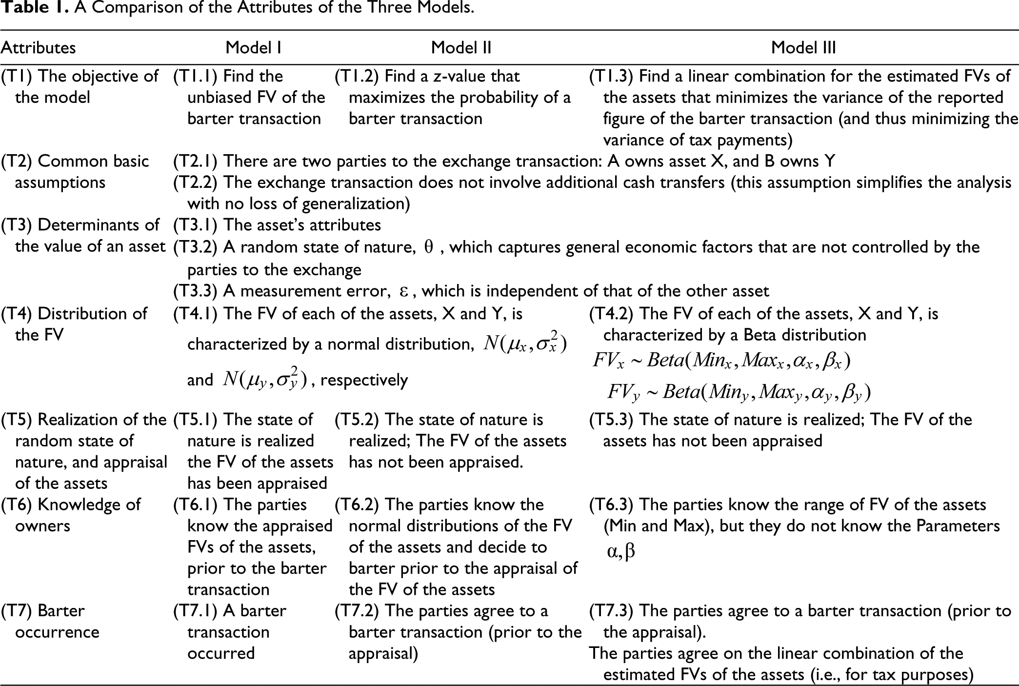
The models share some common basic assumptions, including the determinants of the asset value, but differ from each other with respect to the objective of the model, the assumption regarding the distribution of the FV, the assumption regarding the realization of the random state of nature, and the assumption regarding the knowledge of the owners. Table 1 summarizes the characteristics of the three models.

Table 1.

A Comparison of the Attributes of the Three Models.

Attributes	Model I	Model II	Model III
(T1) The objective of the model	(T1.1) Find the unbiased FV of the barter transaction	(T1.2) Find a z-value that maximizes the probability of a barter transaction	(T1.3) Find a linear combination for the estimated FVs of the assets that minimizes the variance of the reported figure of the barter transaction (and thus minimizing the variance of tax payments)
(T2) Common basic assumptions	(T2.1) There are two parties to the exchange transaction: A owns asset X, and B owns Y
	(T2.2) The exchange transaction does not involve additional cash transfers (this assumption simplifies the analysis with no loss of generalization)
(T3) Determinants of the value of an asset	(T3.1) The asset’s attributes
	(T3.2) A random state of nature, $θ$ , which captures general economic factors that are not controlled by the parties to the exchange
	(T3.3) A measurement error, $ε$ , which is independent of that of the other asset
(T4) Distribution of the FV	(T4.1) The FV of each of the assets, X and Y, is characterized by a normal distribution, $N (μ_{x}, σ_{x}^{2})$ and $N (μ_{y}, σ_{y}^{2})$ , respectively		(T4.2) The FV of each of the assets, X and Y, is characterized by a Beta distribution
			$F V_{x} ~ Beta (Mi n_{x}, Ma x_{x}, α_{x}, β_{x})$ $F V_{y} ~ Beta (Mi n_{y}, Ma x_{y}, α_{y}, β_{y})$
(T5) Realization of the random state of nature, and appraisal of the assets	(T5.1) The state of nature is realized the FV of the assets has been appraised	(T5.2) The state of nature is realized; The FV of the assets has not been appraised.	(T5.3) The state of nature is realized; The FV of the assets has not been appraised
(T6) Knowledge of owners	(T6.1) The parties know the appraised FVs of the assets, prior to the barter transaction	(T6.2) The parties know the normal distributions of the FV of the assets and decide to barter prior to the appraisal of the FV of the assets	(T6.3) The parties know the range of FV of the assets (Min and Max), but they do not know the Parameters $α, β$
(T7) Barter occurrence	(T7.1) A barter transaction occurred	(T7.2) The parties agree to a barter transaction (prior to the appraisal)	(T7.3) The parties agree to a barter transaction (prior to the appraisal).
			The parties agree on the linear combination of the estimated FVs of the assets (i.e., for tax purposes)

Common Assumptions and the Determinants of the Assets’ Value

The first two basic assumptions are straightforward. The restriction on cash transfer (T2.2) is a technical one. Both asssumptions simplify the analysis with no loss of generalization.

Of the three determinants of the value of an asset, two affect the demand for the asset and its market value. The asset’s attributes (T3.1) refer to its inherent characteristics, for example, the location of an apartment, the quality of its neighborhood, its size, and fixtures. The random state of nature (T3.2) captures general economic factors over which the parties have no control. For example, a threat by the Iranian Government to block the Strait of Hormuz may push up oil prices and push down the value of an apartment located in a distant suburb. The third, a technical property, states that the measurement error, $ε$ , of asset X is independent of that of asset Y.

Model I

The objective of Model 1 is to find the unbiased FV of the barter transaction. We prefer this statistic because an unbiased estimator possesses the desired property of having a value, which on the average, equals that of the population. For Model I, we add two specific assumptions:

The FV of each of the assets, X and Y, is characterized by a normal distribution, $N (μ_{x}, σ_{x}^{2})$ and $N (μ_{y}, σ_{y}^{2})$ , respectively.

First, the state of nature is realized. Second, the FV of the assets is appraised and the parties are informed of the assets’ FV. Third, the Barter occurred.

Figure 1 depicts a time analysis of the elements of Model 1.

Figure 1.

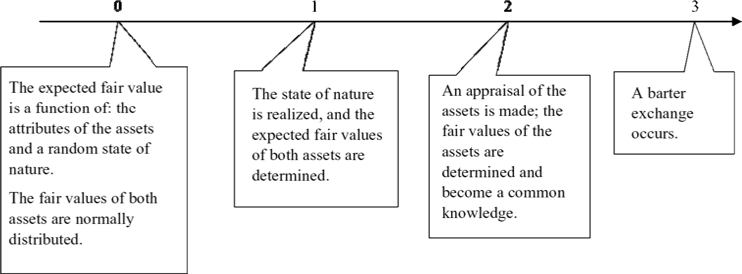
Time analysis of the elements of Model I.

Given our assumption that the parties agree to a barter exchange, without equalizing cash payments, we may deduce that the FV of both assets is equal, such that $F V_{x} = F V_{y}$ and $F V_{z} = F V_{x} = F V_{y}$ , where $F V_{z}$ denotes the FV of both assets.

Result 1

Under the above assumptions, $F V_{z}$ has also a normal distribution, $F V_{z} ~ N (μ_{z}, σ_{z}^{2})$ and the unbiased mean of the FV of the barter equals $μ * = \frac{\frac{1}{σ_{x}^{2}} μ_{x} + \frac{1}{σ_{y}^{2}} μ_{y}}{\frac{1}{σ_{x}^{2}} + \frac{1}{σ_{y}^{2}}}$ .

Proof: See Appendix A for the proof of Result 1.

For example, assume that the following are the estimated FV and variances of two non-monetary assets, X and Y, in a barter transaction $μ_{x} = 20, μ_{y} = 25, σ_{x} = 1 and σ_{y} = 2$ . The unbiased estimated FV of the exchange is

\frac{σ_{y}^{2} μ_{x} + σ_{x}^{2} μ_{y}}{σ_{x}^{2} + σ_{y}^{2}} = \frac{4 \times 20 + 1 \times 25}{1 + 4} = \frac{105}{5} = 21 .

If in a barter exchange, the owner of asset X adds the amount of d dollars to the owner of asset Y, then the unbiased mean of the FV of the barter equals $μ * = \frac{\frac{1}{σ_{x}^{2}} (μ_{x} + d) + \frac{1}{σ_{y}^{2}} μ_{y}}{\frac{1}{σ_{x}^{2}} + \frac{1}{σ_{y}^{2}}} .$ ¹

Model II

The objective of Model II is to find a value $z$ that maximizes the probability of a barter transaction (T1.2). The model portrays a common reality in which the parties to a barter transaction face two alternatives: (a) sell-and-buy or (b) barter. In a sell-and-buy dual-transaction, each of the parties sells the asset he owns and purchases the asset he desires. In a barter transaction, each of the parties exchanges the asset he owns for the asset he desires.

The two alternatives differ from each other in a number of respects, most important of which is, probably, the risk that each of the parties assumes. In the sell-and-buy alternative, because neither the owned, nor the desired asset, has a price tag, each of the parties faces the risk of selling the asset he owns at a low price and purchasing the asset he desires at a high price. In the barter transaction, the parties avoid the above risks.

We define the “FV of the exchange” ( $F V_{z}$ ) to be the unique value, $z$ , which maximizes the probability that both parties agree to sell the asset they, respectively, own for $z$ dollars and to buy, for the very same amount, the asset they, respectively, desire. In other words, this $z$ , maximizes the probability of barter. We show that the “two transactions approach” yields a FV of the exchange, $F V_{z}$ , which equals approximately the weighted average of X and Y, weighted inversely to their variances.

For Model II, we add the following specific assumptions:

The FV of each of the assets, X and Y, is characterized by a normal distribution, $N (μ_{x}, σ_{x}^{2})$ and $N (μ_{y}, σ_{y}^{2})$ , respectively (T4.1).

First, the state of nature is realized. Second, each of the parties knows the normal distributions of the FV of the both assets, the one he owns and the one he desires, f(x) and g(y), respectively, and third, the parties decide to barter prior to the appraisal of the FV of the assets.

Given our assumption that the parties agree to a barter exchange, without equalizing cash payments, we may deduce that the FV of both assets is equal, such that $F V_{x} = F V_{y}$ , and $F V_{z} = F V_{x} = F V_{y}$ .

Figure 2 depicts a time analysis of the elements of Model II.

Figure 2.

Time analysis of the elements of Model II.

We now analyze the logic of the parties to consume the barter with reference to “two transaction approach.” Party A fears that if he sells his asset X, he will receive, with probability $F (z)$ , less than $z$ dollars and if he buys asset Y he will pay, with probability $1 - G (z)$ , more than $z$ dollars. Therefore, the higher is $F (z) (1 - G (z))$ , the higher is the probability that Party A agree to barter. Similar argument holds for Party B.

We now define $z$ to be the price that maximizes the overall probability that both parties will agree to the exchange:

z = \arg max {P = F (z) (1 - F (z)) G (z) (1 - G (z))} .

The second model produces results similar to those of the first model; these results are valid prior to asking for an appraisal of the exchanged assets.

Result 2

If the FV of asset X is normally distributed $N (μ_{x}, σ_{x}^{2})$ and the FV of asset Y is normally distributed $N (μ_{y}, σ_{y}^{2})$ , then $z * \approx \frac{σ_{y}^{2} μ_{x} + σ_{x}^{2} μ_{y}}{σ_{x}^{2} + σ_{y}^{2}} .$

Proof: See Appendix B for the proof of Result 2.

Example: If the FV of assets X and Y are normally distributed and their means and variances are given as follows:

	Asset A	Asset B
M	20	25
SD	3	1.5

then $z * = 24.03$ and $\hat{z} = 24$

Where $z *$ is the “FV of the Exchange” as calculated by our model, and $\hat{z}$ is the theoretical weighted average of the means estimations, weighted inverse to their variances.

Model III

The objective of Model III is (T1.3) to find a linear combination for the estimated FVs of the assets that minimizes the variance of the reported figure of the barter transaction.

The logic of this model stems from reality, as follows. Assume that tax authorities require that parties to barter record the transaction at an identical value. As the transaction’s value may affect taxes and the parties to barter may agree on a value that minimizes total tax payments, the tax authorities, in our setting, require that the parties use independent professional assessment of the assets’ FV, and agree on a predetermined linear combination method for weighting the FVs.

The parties, who must record the barter at a one agreed-on figure, would like, obviously, to minimize the expected tax payments. Nonetheless, they do not know the expected FV, and have no control over the independent assessors. Thus, as an attainable secondary objective, they seek to minimize the variance of their tax payments. The model shows that the linear combination, which minimizes the variance of the recorded figure, is the values provided by the independent assessors weighted by the inverse of the variance of the assessed FVs.

For Model III, we add the following specific assumptions:

The FV of each of the assets, X and Y, is characterized by a Beta distribution, $F V_{x} ~ Beta (Mi n_{x}, Ma x_{x}, α_{x}, β_{x})$ , and $F V_{y} ~ Beta (Mi n_{y}, Ma x_{y}, α_{y}, β_{y})$ ;

The parties know the range of FV of the assets (Min and Max), but they do not now the parameters $α, β$ ;

First, the state of nature is realized. Second, the parties agree to a barter transaction (prior to the appraisal), and on the linear combination of the estimated FVs of the assets (i.e., for tax purposes).

The standard deviation of the Beta distribution equals $\frac{Max - Min}{6}$ . Because both parties know the range of the distributions, they know its variance and standard deviation.

Figure 3 depicts a time analysis of the elements of Model III.

Figure 3.

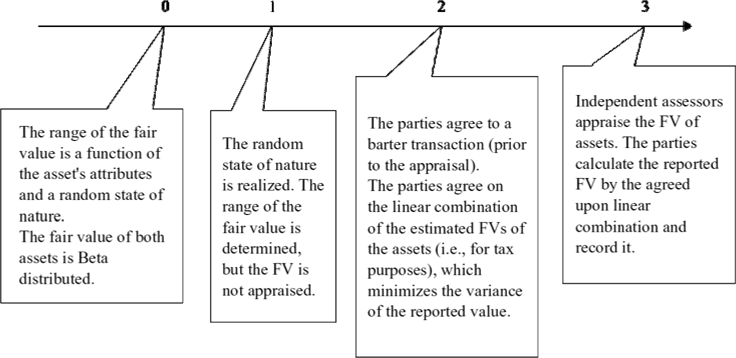
Time analysis of the elements of Model III.

Result 3

The linear combination that minimizes the variance of the estimated FV of the barter is when the weights are the inverse of the variance.

Proof: See Appendix C for the proof of Result 3.

For example, assume that the FV estimates are $F V_{x} = 20, F V_{y} = 30 and σ_{x} = 2, σ_{y} = 4$ , the estimated FV of the exchange is $\frac{16 \times 20 + 4 \times 30}{4 + 16} = \frac{440}{20} = 22$ .

It is important to note that the procedure for calculating the estimated FV of the barter, given the Beta distribution, is quite simple. Assume that the FVs of assets A and B have the following minimum and maximum values: A = (Min $100; Max $150); B = (Min $110, Max 135). The independent assessors provide the following appraisals for A = $120, and for B = $130.

Because the ratio of the standard deviations is equal to the ratio of the ranges, we obtain that $\frac{Var (F V_{x})}{Var (F V_{y})} = {(\frac{50}{25})}^{2} = 4$ . Therefore, we combine the estimates received from the assessors by giving asset X a weight of 1 and asset Y a weight of 4. The estimated FV of the barter, therefore, is $\frac{1 \times 120 + 4 \times 130}{5} = 128$ dollars.

Contribution, Summary, and Conclusion

General Model for Estimation of FV in an Exchange Transaction

This article contributes to the accounting body of knowledge in two ways: major and adjacent. The major contribution is a general standard for estimating cost in exchange transactions that is applicable to all types of exchanges. It includes, for example, the purchase and sale of assets, the settlement of debt, equity-based payments, and of course, the accounting for non-monetary asset transactions.

The idea of one general standard for measuring cost in transactions of various characteristics is far reaching. It introduces consistency and comparability, reduces complication, and increases comprehension of accounting standards. Incidentally, it points out the deficiencies of current standard in measuring cost, and enhances the study of accounting theory. The following discussion details the adjacent contributions.

Bridging the Gap Between Entry and Exit Prices

Following Sprouse and Moonitz (1962), Chambers (1965), and Sterling (1970), the FASB defines entry price (cost) and exit price (the FV) and emphasizes that they are different (FASB, 2006, para. 16). This article demonstrates that entry and exit prices are special cases of FV estimation in an exchange transaction. In the case of a purchase transaction, where the payment is in cash, the entry price equals “the price paid to acquire the asset.” This is so because the estimated variability of cash is zero; and thus, regardless of the estimated FV and variability of the acquired asset, the weighted average of the both FV estimations, equals the cash payment.

The following example clarifies this point. Assume that an entity purchases an asset for $20 in cash. The FV of the asset acquired has a mean of $25 and a variance of $4. The “fair value” of the exchange transaction, as prescribed by the proposed model, is

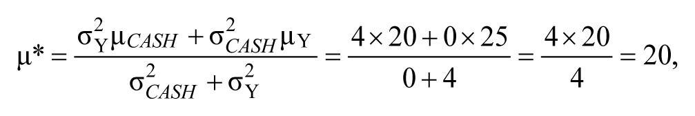
μ * = \frac{σ_{Y}^{2} μ_{CASH} + σ_{CASH}^{2} μ_{Y}}{σ_{CASH}^{2} + σ_{Y}^{2}} = \frac{4 \times 20 + 0 \times 25}{0 + 4} = \frac{4 \times 20}{4} = 20,

and it equals the entry price.

Inconsistencies Among the FASB’s Requirements for Measuring Cost

The APB, in Opinion 29 (1973, para. 18), prescribes the general rule, that the FV of the given-up asset (the exit price) will serve as the cost of the acquired asset. In contrast, in Opinion 16 (APB, 1970, para. 67, c), which refers to issuance of shares in acquisition of assets, the APB recommends the use of FV of the acquired asset for recording its cost (entry price). In other words, a firm must record shares issued in an asset acquisition at the FV of the acquired asset (APB, 1970, para. 67, c).

When we use the framework of Opinion 29 (APB, 1973) for analyzing this rule, it becomes clear that the APB regards the FV estimation of the acquired asset to be more reliable than that of the issued shares. Although it is possible to suggest reasons for the Board’s stance (i.e., reducing potential window dressing), this rule contradicts the Board’s own model for cost determination. A reference to FAS 157 (FASB, 2006, paras. 22-25) clarifies, nonetheless, that in many cases, FV estimations of issued shares are quality inputs of Levels 1 and 2.

In our opinion, the control over potential window dressing must not affect accounting principles. Therefore, we suggest replacing the current APB approach with the general method of measuring cost proposed here.

Inconsistencies Among the IASB’s Requirements for Measuring Cost

The IASB, in IAS 16 (IASB, 1993b, paras. 24, 26), prescribes that the cost of an acquired asset in a non-monetary exchange transaction is the FV of the surrendered asset. In contrast, the Board, in IAS 18 (IASB, 2006), which focuses on revenue, imposes the opposite rule in the case where a firm purchases fixed assets for inventory. The Board states, as a general rule: “Revenue shall be measured at the FV of the consideration received or receivable” (IASB, 2006, para. 9). The application of this rule to an exchange of inventory for a non-monetary means measuring cost at the FV of the acquired asset.

These contradicting measurement rules may result from the differing perspectives regarding cost-measurement and revenue-recognition. Nonetheless, this does not justify the contradicting rules. A consistent application of the method for cost estimation, which this article proposes, resolves this and similar inconsistencies.

It is interesting to note that U.S. GAAP (Generally Accepted Accounting Principles) do not have this internal inconsistency. The APB (1973, para. 7) establishes that “exchange of product held for sale in the ordinary course of business (inventory) for dissimilar property as a means of selling the product to a customer” must be recorded at the FV of the inventory sold (APB, 1973, para. 7, example a).

A similar inconsistency exists in IFRS 2 Share-Based Payment (IASB, 2004). In contrast to the measurement requirements set by IAS 16 (IASB, 1993), IFRS 2 determines that in general,

For equity-settled share-based payment transactions, the entity shall measure the goods or services received, and the corresponding increase in equity, directly, at the fair value of the goods or services received. (IASB, 2004, para. 10)

This inconsistency too does not prevail in U.S. GAAP. FAS 123R (FASB, 2004), which concerns share-based payments, requires the use of the more reliable FV estimate between the given-up equity instruments and the acquired asset. When the share-based transaction occurs between the entity and its employees, the FV of the shares transferred is clearly preferable (FASB, 2004, para. 7).

Summary

The main objective of this article is to offer a model for FV estimation that faithfully represents a non-monetary exchange transaction. We show that this value is a weighted average of the FV estimations of the assets exchanged, where the weights are the inverse of the asset’s variances. It is an unbiased mean estimator of the barter’s FV, and it depicts the reality of the parties’ agreement to a non-monetary barter with no adjusting cash transfers. We use three models that portray different situations to support and provide robustness for our proposal.

Our model utilizes available, currently discarded, information, as encouraged by the FASB (2006), and thus, improves the estimated value; it prevents the use of extreme values for recording cost (either the estimate of the FV of the surrendered asset or the FV of the acquired asset); it also precludes a potential inconsistency of cost recording, which may arise where the FV estimations of both assets to the transaction, are of the same level of reliability. In the latter case, under current rules, each of the parties uses a different cost figure.

The model bridges the gap between entry price (cost) and exit price (FV). It shows that entry price and exit price are special cases of the general rule of FV estimation, where one of the assets is cash. The model, thus, eliminates the current dichotomy of monetary and non-monetary exchange transactions. More so, the model fits many types of exchanges. Its adoption will result in one accounting standard for any type of exchange transaction.

Applying the model in real cases is practical and quite simple. It does not require a full knowledge of the probability distributions of the FV of the exchanged assets. It is sufficient to elicit from the owners (or appraisers) the following information: (a) the most likely value of the asset and (b) a range that captures the FV of the asset with a high probability (for instance, 99%). Because the range linearly relates to the standard deviation, the ratio of the ranges of the estimated FVs of the two assets provides a good estimate of the ratio of the two standard deviations. Given this information, one can easily calculate the weighted average as suggested by the model.

Finally, the proposed model may enhance uniformity and improve comparability of accounting reports.

Footnotes

Appendix A

Appendix B

Appendix C

Declaration of Conflicting Interests

The author(s) declared no potential conflicts of interest with respect to the research, authorship, and/or publication of this article.

Funding

The author(s) received no financial support for the research and/or authorship of this article.

Notes

Author Biographies

Benzion Barlev, PhD, is Head of the Accounting Department, The Center for Academic Studies in Or Yehuda, and Prof. (Emeritus), School of Business Administration, The Hebrew University of Jerusalem, Mount Scopus, Jerusalem, Israel.

Joseph Tzur, PhD, is a Senior Lecturer of Accounting at Ono College and Ruppin Academic Center, Israel.

References

Accounting Principles Board. (1970). Business combination (APB Opinion 16). New York, NY: AICPA.

Accounting Principles Board. (1973). Accounting for nonmonetary transactions (APB Opinion 29). New York, NY: AICPA.

Chambers

R. J.

(1965). Accounting, evaluation and economic behavior. Englewood Cliffs, NJ: Prentice Hall.

DeGroot

H. M.

(1970). Optimal statistical decisions. New York: McGraw-Hill.

Financial Accounting Standards Board. (2004). Share-based payment (FASB Statement No. 123R). Norwalk, CT: Author.

Financial Accounting Standards Board. (2005). Accounting changes and error corrections a replacement of APB Opinion No. 20 and FASB Statement No. 3 (Statement No. 154). Norwalk, CT: Author.

Financial Accounting Standards Board. (2006). Fair value measurements (Statement No. 157). Norwalk, CT. Author.

International Accounting Standards Board. (1993a). Accounting policies, changes in accounting estimates and errors (IASB Standard No. 8). London, England: IASCF.

International Accounting Standards Board. (1993b). Property, plant and equipment (IASB Standard No. 16). London, England: IASCF.

10.

International Accounting Standards Board. (1993c). Revenue (IASB Standard No. 18). London, England: IASCF.

11.

International Accounting Standards Board. (2004). Share-based payment (IASB Reporting Standard No. 2). London, England: IASCF.

12.

Hendriksen

E. S.

van Breda

M. F.

(1982). Accounting theory (5th ed.). Homewood, IL: Irwin.

13.

Most

(1982). Accounting theory (2nd ed.). Columbus, OH: Grid Publishing.

14.

Sprouse

R. T.

Moonitz

(1962). A tentative set of broad accounting principles for Business Enterprises (Accounting Research Study No. 3). New York, NY: AICPA.

15.

Sterling

R. R.

(1970). Theory of the measurement of enterprise income. Kansas City: University of Kansas Press.

A General Model for Cost Estimation in an Exchange