Sage Journals: Discover world-class research

Abstract

It is generally accepted that interviewers have a considerable effect on survey response. The difference between response success and failure does not only affect the response rate, but can also influence the composition of the realized sample or respondent set, and consequently introduce nonresponse bias. To measure these two different aspects of the obtained sample, response propensities will be used. They have an aggregate mean and variance that can both be used to construct quality indicators for the obtained sample of respondents. As these propensities can also be measured on the interviewer level, this allows evaluation of the interviewer group and of the extent to which individual interviewers contribute to a biased respondent set. In this article, a procedure based on a multilevel model with random intercepts and random slopes is elaborated and illustrated. The results show that the procedure is informative to detect influential interviewers with an impact on nonresponse basis.

Keywords

response propensities nonresponse bias nonresponse contrast random intercepts random slopes interviewer effects

Introduction

It has become common knowledge that interviewers play a prominent role in the course of contact with respondents and heavily influence the process of gaining survey cooperation (see, for example, Campanelli & O’Muircheartaigh, 1999; Durrant, Groves, Staetsky, & Steele, 2010; Durrant & Steele, 2009; Pickery & Loosveldt, 2002). A large volume of relevant research points to differences in response rates between interviewers as being a result of varied interviewer characteristics, or their behavior during doorstep interaction. Multilevel models allowing for random intercepts usually take into account the findings of this type of research. However, literature concerning interviewer effects primarily focuses on differences in response rates, ignoring the possibility that interviewers can also contribute differently to the composition of the realized respondent set. If this is the case, interviewers may have an effect on nonresponse bias, as their success rates will also differ in respect of specific sample profiles. For example, supposing that on average slightly more females than males participate in a survey, it is easy to imagine that the gender ratio may not necessarily remain constant between all interviewers. Some interviewers may be more inclined to engage with women than the average of all the interviewers. If such female-biased interviewers are systematically deployed more frequently, the gender contrast will be aggravated. However, deploying more interviewers who are gender-neutral will lessen the risk of nonresponse bias, at least with regard to gender.

Current research on nonresponse bias has brought attention to the fact that a single-minded focus on response rates alone can sometimes be misleading (see, for example, Biemer & Lyberg, 2003; Groves, 2006; Groves & Peytcheva, 2008). A higher response rate limits the degree to which nonresponse damage can be manifested. However, without knowing the magnitude of the difference between respondents and nonrespondents, response rate is only a weak predictor of nonresponse bias. Furthermore, as survey objectives are typically aimed at the maximization of response rates, the contrast between respondents and nonrespondents may be overlooked, with the result that the pursuit of response rate only generates more of the same type of respondents. Through this mechanism, the declining group of nonrespondents becomes more atypical and even more nonresponse bias may be induced, despite the higher response rate. Particularly in face-to-face surveys, such problems are even more troublesome, as interviewers have more exclusive control over the selection and treatment of sample cases. In this regard, Peytchev, Riley, Rosen, Murphy, and Lindblad (2010, p. 22) stated that interviewers “are often evaluated on their response rates and not on nonresponse bias in their sample. Thus, interviewers can be expected to direct greater effort to sample members they deem more likely to participate regardless of potential nonresponse bias.” From these observations, it seems worthwhile to assess the effect on nonresponse bias of the variability within the interviewer group. This article primarily attempts to develop a procedure to measure these interviewer-specific biases.

Essentially, our procedure expands on the aforementioned random intercepts model, using random slopes with regard to the auxiliary variables. These auxiliary variables are available for every sample or population element and have a substantive relevance. This means that these variables are related to the target variables, and aim to predict the propensity of survey participation. Given these response propensities, some quality indicators can be derived in respect of the obtained sample or the respondent set: the propensity mean obviously reflects the overall response rate and the variability of propensities can be used to construct contrast and bias estimates. Interviewers who have individual slopes that are close to 0 with regard to these auxiliary variables will generate less propensity variance and can consequently be expected to contribute less to response-set contrast and/or bias. It is clear that the ability to measure this interviewer immunity depends strongly on the available auxiliary information.

First, we briefly discuss the concept of nonresponse bias to measure the quality of an obtained sample or respondent set, based on response propensities. Then, this quality framework is further developed toward the interviewer level using multilevel modeling, including random intercepts and slopes. Finally, an empirical illustration is given, based on data from the Flemish Housing Survey of 2005-2006.

Review of Sample Quality Indicators Based on Estimated Response Propensities

In survey research, the terminology addressing survey quality covers many aspects, both at the level of the sample construction (coverage error, sampling error, and nonresponse error) and at the level of the obtained answers to the questionnaire. In this article, we deal only with nonresponse error and consider the potential damage or bias to a realized respondent set as the most important aspect of quality. First, we define some sample quality indicators and in the next section, the procedure to assess interviewer effects on these indicators is introduced.

Nonresponse bias can be seen as the difference between the respondent mean and the complete sample mean with respect to a target variable y. We refer to the difference between respondents and nonrespondents on the mean of the target variable y as “the contrast.” Usually, the interest concerns more than a single target survey variable. Therefore, we concentrate more on the maximal bias than on the actual bias that needs to be measured separately for each target variable.

The quality framework deployed here starts from the existence of an individual response propensity. The estimates of these response propensities are derived from a response propensity model. It is assumed that the model is correctly specified. A response propensity can be defined as $ρ_{X} (x_{i}) = E (R_{i} = 1 | x_{i})$ , or the expectation of the response of unit i, conditional on the information of the auxiliary variable X (Little, 1986, 1988; Shlomo, Skinner, Schouten, Bethlehem, & Zhang, 2009; Bethlehem, Cobben, & Schouten, 2011). Auxiliary variables are available for all the sample units. Examples of auxiliary variables are demographic characteristics such as age, gender, and marital status. This notion of response propensity reflects the viewpoint that responding to a survey request is largely a manifestation of the respondent’s latent propensity ρ_i, or as Schouten, Cobben, and Bethlehem (2009) posited “a biased coin that a unit carries in a pocket” (p. 103). From this viewpoint, nonresponse bias for ${\bar{y}}_{r}$ (unadjusted respondent mean) can be written as (see, for example, Bethlehem, 2009)

b i a s ({\bar{y}}_{r}) ≅ \frac{c o r r_{ρ y} σ_{ρ} σ_{y}}{\bar{ρ}} .

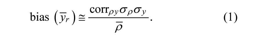
The bias is a function of the correlation between response propensities and the target variable ${corr}_{ρ y}$ (controlling for other factors, stronger correlations lead to more bias), the standard deviation of response propensities $σ_{ρ}$ (controlling for other factors, larger variance produces more bias), the standard deviation of the target variable $σ_{y}$ , and the response rate $\bar{ρ}$ (controlling for other factors, higher response rates generate less bias). The expression makes clear that there is no simple relationship between rate and bias and that an increase in the response rate does not automatically result in less bias.

Under the assumption that the target variable y has first been standardized and there is a perfect correlation between the target variable y and the estimated propensities, we obtain

| b i a s ({\bar{y}}_{r}) | < \frac{σ_{ρ}}{\bar{ρ}} .

Equation 2 can also be understood as the maximal possible absolute bias, or the maximal possible absolute difference between respondents and the complete set of respondents and nonrespondents. Based on Equation 2, a measurement expressing the maximal absolute contrast between the respondents and the nonrespondents can also be determined (in general, bias = nonresponse rate × contrast → contrast = bias/nonresponse rate):

| {\bar{y}}_{r} - {\bar{y}}_{n r} | < \frac{σ_{ρ}}{\bar{ρ} (1 - \bar{ρ})} .

In Equation 3, $(1 - \bar{ρ})$ is the nonresponse rate and in both Equations 2 and 3, the basic components are the mean propensity $\bar{ρ}$ , and the standard deviation of the propensities $σ_{ρ}$ . This requires a good set of auxiliary variables $ℵ$ , capable of explaining all the variability between the true individual response propensities. In practice, however, the set of auxiliary variables is restricted to $a u x \subset ℵ$ . Therefore, it is expected that nonresponse models based on auxiliary variables are usually misspecified. Therefore, the obtained bias of the estimate based on the propensity models is not general, but conditional on the available and selected auxiliary variables in the models.

One basic approach of estimating response propensities is the use of multiple logistic regression (other link functions such as probit can also be used):

l o g i t [P (r_{i} = 1)] = α + \sum_{a u x = 1}^{q} (β_{a u x}) x_{a u x, i} .

In this expression, the probability is modeled that someone is a respondent (r_i = 1), given an intercept α and a β_aux, with one β for each auxiliary variable in the model. The auxiliary variables in Model 4 must take into account that response propensities do not only originate from the preeminence of the individual sample cases but also result from the interplay between the sample cases and the way they are treated during the contact process. Therefore, the auxiliary variables can also be derived from social environmental variables, information recorded in paradata about the doorstep interaction, and other information from call records. This is in line with the conceptual framework for survey participation put forward by Groves and Couper (1998) and Dalenius (1983), who argued that the reaction to a survey request is determined by the combination of the social environment, the survey design, and the interaction between the interviewer and interviewee. Notably, this interaction during the fieldwork makes it clear that propensities depend, among other determinants, on how sample cases are treated by their interviewers. Relevant contact-phase treatment variables might include the number of contact attempts devoted to the sample units, the contact modes, the doorstep reasoning techniques, and so forth. Whenever interviewers deploy divergent mixes of contact strategies, the resulting response propensities within their subsamples can consequently be affected with regard to the mean and variance structures.

Multilevel Models and the Assessment of Interviewer Effects on Nonresponse: A Random Slope Extension

During recent decades, multilevel models have been used to assess interviewer effects on response, contact, and cooperation rates. These interviewer effects are well documented. As examples, we mention some relevant papers and results. Based on the results of a cross-classified multilevel model, O’Muircheartaigh and Campanelli (1999) concluded that variance created by systematic differences between interviewers is greater than the variance between geographic areas. Their results further suggest that interviewers who are good at reducing household refusals are also good at reducing household noncontact. Pickery and Loosveldt (2002) found interviewer effects with respect to cooperation rates and contact rates. In their analysis, they also found that both interviewer components correlate positively. Similar conclusions were drawn by Durrant and Steele (2009). Durrant et al. (2010) found that response success depends on interviewers’ confidence and attitudes toward persuading reluctant respondents. They also found support for the theory of liking: Similarity between interviewers and sample cases (e.g., in respect of gender and educational level) generate higher survey cooperation. The impact of the variance in nonresponse error between interviewers on the interviewer effects on substantive variables was studied by West and Olson (2010). In a computer-assisted telephone interviewing (CATI) survey, they found evidence that interviewer-related variance on some key survey items may be due to nonresponse error variance. The results shown in West and Olson’s paper make clear that interviewers “select” different types of respondents and as a consequence, they are responsible for nonresponse bias. Although one must be aware of the possible entanglement of interviewer effects and area effects, previous research has shown that a substantial amount of cluster and/or area-related variance in respect of both response rates (Campanelli & O’Muircheartaigh, 1999) and the recording of survey answers once cooperation has been established (Schnell & Kreuter, 2005; West, Kreuter, & Jaenichen, 2013), can be attributed to the interviewer. Therefore, interviewers are responsible for a larger part of the homogenizing effect than is spatial clustering.

In the next section, we specify a multilevel model to assess interviewer effects on nonresponse bias.

When only investigating interviewer effects on the response rate, the following multilevel model could be used:

logit [P (r_{i j} = 1)] = α_{j} + \sum_{a u x = 1}^{q} (β_{a u x}) x_{a u x, i j} .

The necessary components for this model are as follows:

A 0-1 response indicator r_i for each (non)responding sample unit i.

A set of q relevant auxiliary variables available for each (non)responding sample unit i.

A vector indicating which interviewer j has been assigned to which (non)responding sample unit i.

A special case of this general model is a model without independent variables (null model):

logit [P (r_{i j} = 1)] = α_{j} .

Both models measure the probability of responding positively to a survey request. For each interviewer j, α indicates the intercept of a logistic regression that is now interviewer specific (α_j = random intercept). The second model is the null model with only an interviewer-specific intercept (random intercept) that expresses the response rate for each interviewer. This model can be considered as a specification of the first model (which also includes auxiliary variables, for example, age, gender, area information, or type of housing). The interviewer-specific intercept can be expressed as a general overall response rate γ₀, which is the same for each interviewer, and an interviewer-specific component of the intercept: α_j = γ₀ + µ_0j. The interviewer-specific component is the interviewer’s deviation from the overall response rate.

In a random intercepts model with auxiliary variables (Model 5), these variables serve to partially control-out the effects of the nonrandom assignment of interviewers to sample cases. Note that in this model (5), the slopes of the auxiliary variables β_aux are not interviewer specific. These parameters are fixed and are the same for each interviewer. Therefore, Model 5 is one with only a random intercept. By using this model, the resulting response rates are more comparable between interviewers. The validity of the comparison greatly depends on both the availability of relevant auxiliary variables and the external heterogeneity of the clusters to which interviewers are assigned.

In Model 7, we specify a random intercept and a random slope model. In this model, each interviewer has a specific intercept and a specific slope for each auxiliary variable:

l o g i t [P (r_{i j} = 1)] = α_{j} + \sum_{a u x = 1}^{q} (β_{a u x, j}) x_{a u x, j, i} .

The intercept and slope estimates per interviewer are $α_{j}$ and $β_{a u x, j}$ . Alternatively, $α_{j}$ and $β_{a u x, j}$ can also be decomposed into the fixed parts $γ_{0}, γ_{1}, \dots, γ_{q}$ , which are the same for all interviewers, and the random parts $u_{0 j}, u_{1 j}, \dots, u_{q j}$ , which are specific to each interviewer. Therefore, at the interviewer level there is variance for the intercept $(σ_{μ_{0}}^{2})$ and the slopes ( $σ_{μ_{1}}^{2}; \dots$ ). These variances express the differences between interviewers in specific parts of the response rates (random intercepts) and the differences in the effects of the auxiliary variables (random slopes). When these variances are significantly different from 0, there are significant differences between interviewers. Based on the results of a random slope and random intercept model, it is also possible to calculate and evaluate the correlation between the interviewer-specific part of the intercept and the slope.

In the most optimal situation, there is no effect of the auxiliary variables. This means that both fixed $γ_{1}, γ_{2}, \dots, γ_{q}$ and random $u_{1 j}, u_{2 j}, \dots, u_{q j}$ effects of the auxiliary variables are absent, suggesting that there are no independent variables that are responsible for the divergence of response propensities. After all, equality of response propensities leads to representative and thus unbiased respondent sets (Schouten et al., 2009). In addition, γ₀ (the fixed part of the intercept) should be as high as possible (= high response rate). Moreover, low or no variation in the interviewer-specific intercepts is desirable, meaning that the response rates for the interviewers are similar. This indicates that interviewer assignment in the field is not responsible for bias issues (e.g., sending high response rate interviewers to a selective group of responsive sample cases). Random slopes indicate that some interviewers deviate from the fixed effect of the variable on survey participation. This is an indication that nonresponse occurs differently, depending on the interviewer. The worst-case scenario combines strong fixed effects of the auxiliary variables with the absence of random slopes: response propensities are related to the auxiliary variables and the effect of these variables is the same for all the interviewers. As a consequence, there are no interviewers with higher response rates, in particular, groups that can be used to alter the low response rates of other interviewers in these groups. Accordingly, response propensities tend to be different, while no interviewer is in the position of altering low response rates in specific groups.

Model 7 permits obtaining interviewer-specific intercepts and a set of interviewer-specific slopes with respect to the auxiliary variables. A first method involves the evaluation of the intercepts (higher values are preferable) and slopes (values closer to 0 are better). The disadvantage of this method is the computational and interpretative complexity when using a large number of auxiliary variables. Therefore, a selection of substantively relevant auxiliary variables is recommended. This means that the auxiliary variables are related to the key variables of the survey. It is also important that the effects of these variables are significantly different between interviewers. Moreover, as the intercepts reflect the variation in response rates and the slopes indicate the variation in interviewer-specific contrast, the combination of intercepts and slopes still has to be performed to obtain an interviewer-specific bias indication. We therefore need a way to synthesize all the random parts into one quality framework.

A quality indicator framework based on response propensities probably serves to provide a better accommodation of the evaluative procedure. In the first instance, one could predict a response propensity for each sample case i within interviewer j, using the logistic parameters of interviewer j. This is problematic, because the interviewer-specific samples are not equivalent, so the resulting propensity means and variance depend strongly on the values of the auxiliary variables in that particular interviewer cluster. This obstructs the comparability of response rates, contrasts, and biases between interviewers. Therefore, it is better to use a common set of sample cases, for which response propensities are computed separately for each interviewer. In the illustration further on, we use a complete survey sample. Nevertheless, a second problem needs to be solved. What are termed the empirical Bayes (EB) estimates, obtained from Model 7, are probably biased due to parameter shrinkage (see, for example, Hox, 2002; Raudenbush & Bryk, 2002; Snijder & Bosker, 1999) or partial pooling (Gelman & Hill, 2007). In the case of a separate (logistic) regression being performed for each interviewer, the resulting parameters are probably more variable than their EB counterparts. This is particularly a problem when interviewers have different workloads, and thus different sample sizes. To solve this problem, the interviewer-specific estimates will be a weighted function of the fixed and EB estimates. The properties of the new estimates are discussed and illustrated in the appendix.

Illustration: Flemish Housing Survey 2005-2006

Data

The Flemish Housing Survey was conducted by the Research Network on Sustainable Housing Policy, commissioned by the Housing Policy Department of the Ministry of the Flemish Community. The target population consisted of all private dwellings in Flanders, Belgium. Preceding the actual survey, an evaluation of the quality of the dwellings by experts took place. Ten experts were trained. They worked independent of the interviewers, and their inspections were predominantly based on strongly objectified and prespecified criteria. For this part of the research project, no cooperation (or even contact) was required with the occupants. This technical inspection generated a large inventory of highly relevant auxiliary information about the dwellings, particularly because a subsequent face-to-face survey was carried out with the occupants of the houses. The actual survey screened the profiles, expectations, and needs of the Flemings as housing consumers. The fieldwork period spanned the period from April 2005 to February 2006 and was conducted by 187 experienced (at least 1 year) interviewers, of whom 169 are included in our analysis (assigned to more than three units). Of the 8,400 screened dwellings, some 7,770 (93%) were selected for a face-to-face survey. The selection of cases for attempted contact is believed to have been randomly determined and mainly driven by budget considerations. Within the attempted sample, some elements could not be contacted, despite the mandatory four contact attempts (of which the first needed to be personal, at least one had to be in the evening, and another had to take place at the weekend). In instances where the reference person (usually the head of the family) was deceased, or if the address was not valid, the sample case was considered as ineligible. Availability was decided on if the reference respondent was abroad or simply not at home. Among the eligible respondents, the cooperation rate was about 80% and the response rate 72%. Due to regional clustering, respondents were not randomly assigned to the interviewers.

Because of the screening of the dwellings by experts prior to the actual survey, all dwellings were very well documented in terms of auxiliary data. Note that all available variables at the sample-unit level are housing characteristics. In the analysis later, we only use those auxiliary variables that show explanatory power with respect to the final response outcomes. Therefore, a forward selection procedure is used. Among other items, SCORE_HOUSE, FLAT, and GARAGE are selected (see below for explanations), the width and the year of construction of the building, the gender and age of the family head, the presence of green areas in the neighborhood, the presence of litter in the neighborhood, and the designation of the houses in the area (residential only, commercial area, or rural area) are not selected. A distinction between two classes of auxiliary variables should be mentioned here. The first class is a set of variables that may show some variation between interviewers. The second class refers to municipality-level variables that sometimes may be constant between interviewers. This class of variables is predominantly used to (partially) control out area effects when applying multilevel logistic regression. Obviously, random slopes only apply to the first class of auxiliary variables.

Auxiliary variables measured at the respondent level are as follows:

SCORE_HOUSE: The objectified score of house quality according to the experts’ report. This score is a composite of the experts’ judgments about several exterior deficiencies of the dwelling such as the roof, house front, woodwork, and the presence of broken windows. A higher score means a better quality.

FLAT: 0 = single-unit house; 1 = multiunit house (apartment).

GARAGE: The presence of garage/drive. 0 = no; 1 = yes.

Auxiliary variables measured at the municipality level:

EMPLOYMENT: The number of employed inhabitants per 1,000 inhabitants, aged 15 to 65.

EUROPEAN: The number of European foreigners per 1,000 inhabitants.

WASTE: Kilograms of waste per capita.

Results of a Multilevel Model With Random Intercept and Random Slopes

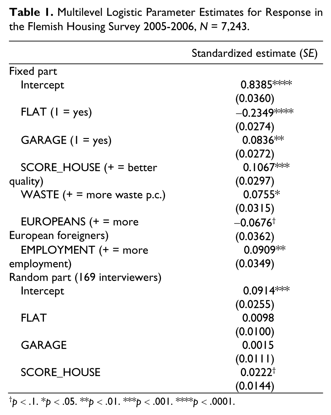
Table 1 presents the results of a logistic multilevel model as expressed in Model 7. Some 527 cases out of 7,770 are omitted, because the respective interviewers were only assigned to a small number of cases (<15) or because of missing values on one of the auxiliary variables. In addition to the random intercepts, the model contains three random slopes on three of the variables (GARAGE, FLAT, and SCORE_HOUSE), controlling for the fixed effects of WASTE, EUROPEANS, and EMPLOYMENT. Due to considerations of parsimony and a lack of well-underpinned hypotheses, we do not include the covariances or correlations between the random intercept and slopes in the model. The model is estimated by means of the SAS GLIMMIX procedure, in which the restricted pseudo-likelihood estimation method is used. Results with regard to the marginal or fixed parameter model show that sample units with a garage and with better housing scores as determined by the experts were more inclined to react positively to the participation request. Those living in apartments were less likely to be included in the obtained sample. In addition, people in municipalities with more waste per capita and higher employment rates tended to be more responsive.

Table 1.

Multilevel Logistic Parameter Estimates for Response in the Flemish Housing Survey 2005-2006, N = 7,243.

	Standardized estimate (SE)
Fixed part
Intercept	0.8385****
	(0.0360)
FLAT (1 = yes)	−0.2349****
	(0.0274)
GARAGE (1 = yes)	0.0836**
	(0.0272)
SCORE_HOUSE (+ = better quality)	0.1067***
	(0.0297)
WASTE (+ = more waste p.c.)	0.0755*
	(0.0315)
EUROPEANS (+ = more European foreigners)	−0.0676^†
	(0.0362)
EMPLOYMENT (+ = more employment)	0.0909**
	(0.0349)
Random part (169 interviewers)
Intercept	0.0914***
	(0.0255)
FLAT	0.0098
	(0.0100)
GARAGE	0.0015
	(0.0111)
SCORE_HOUSE	0.0222^†
	(0.0144)

†

p < .1. *p < .05. **p < .01. ***p < .001. ****p < .0001.

Based on the marginal model alone, it is possible to determine initial response propensities and derive initial estimates of the quality indicators of the obtained sample. The response rate is 0.6952 and the propensity variance equals 0.0065, implying a maximal absolute bias of 0.1160 and a maximal absolute contrast of 0.3804. It is clear that these results are conditional on the specified response propensity model and that the model does not explain survey participation perfectly.

Our interest is focused on the possible variation between interviewers with regard to the intercepts and the slopes of the auxiliary variables in the model. The variance of the random intercepts is significantly different from 0. This means that there are significant differences between interviewers in response rates, which confirms findings in previous research. The random slopes for the auxiliary variables are only significant for SCORE_HOUSE at a level of 0.1. This means that there are significant (p < .1) differences between the interviewers with respect to the effect of SCORE_HOUSE. For the two other auxiliary variables, the effects are not significantly different between interviewers. The fact that only the variance of one slope is significant seems to indicate that the interviewers’ impact on the nonresponse bias is limited. In the next section, we elaborate this first evaluation.

The interviewer-specific parts of the random intercept and the random slopes are used to create interviewer-specific parameters (see the appendix). The distributional aspects of the weighted EB parameters are depicted in Figure 1. The means of the estimates are very close to the estimates provided in Table 1. The variability of the estimates is considerable. This may be partially explained by the inaccuracy of the estimates due to the relatively small sizes of the samples the interviewers were assigned (43 on average).

Figure 1.

Distribution of interviewer-specific parameter estimates (weighted empirical Bayes; 169 interviewers).

Interviewer-Specific Quality Indicators for the Flemish Housing Survey

Having obtained the interviewer-specific parameters, these parameters are applied to the entire sample to calculate the response propensities for each interviewer. The resulting means and variances of these vectors are then used to compute the diverse quality indicators for the obtained sample: the response rate, maximal absolute contrast, and maximal absolute bias.

In Figure 2, the expected response rates and expected maximal absolute contrasts are plotted for each interviewer. As bias is the product of the contrast and the nonresponse rate, the scatterplot of these two indicators is supplemented by two reference lines. A reference line is the product of a specific value of the response rate with a specific value of the contrast to obtain a fixed value for the absolute bias. Figure 2 can be used to identify different types of interviewers based on different combinations of response rate and contrast. Clearly, interviewers who are located in the lower right corner of the graph are to be preferred, as they generate the least bias—resulting from high response rates combined with low maximal absolute contrasts. The lines of equal maximal absolute bias demonstrate the trade-off between the maximization of the response rate, on one hand, and the minimization of the maximal absolute contrast on the other. Interviewers offering the same maximal absolute bias do not necessarily refer to the same values for the building blocks. Some interviewers clearly achieve the highest response rates (80%-90%), but have strongly contrasting values for respondents and nonrespondents, whereas other interviewers showing the same bias level combine lower response rates with low maximal absolute contrasts.

Figure 2.

Expected maximal absolute contrasts and expected response rates for 169 interviewers.

Research that goes beyond the interviewer effects on response rates alone and addresses the interviewer effects on nonresponse bias is hard to find. Estimating rates, contrasts, and biases at the interviewer level may serve in investigating interviewer behavior and its impact on nonresponse. An interesting starting point in this regard is the relationship between interviewer-specific response rates and the contrast between the respective respondents and nonrespondents. A first hypothesis would relate high contrasts to low response rates: Interviewers tend to follow the line of least resistance and try to maximize their response rates (and salary) while minimizing effort, by systematically selecting the cases they deem most likely to participate. If interviewers want to further increase their response rate, they will have to put more effort into sample cases that are harder to convert. However, a competing hypothesis (Peytchev et al., 2010) relates response rates and contrast positively: When increasing the response rate, the set of nonrespondents becomes more atypical and the contrast between respondents and nonrespondents grows. These interviewers would thus cream off only the most promising sample profiles. The correlation between the interviewer response rates and their respective contrasts equals −.02 (p = .87, n = 169), therefore neither of the two competing hypotheses is supported. A hypothesis of a different type links interviewer experience to the reduction of survey bias: More-experienced interviewers may be equipped with better contact strategies and persuasive arguments, so that they grow immune to particular characteristics of the sample members, probably also combined with higher response rates. Another possible explanation for the existence of interviewer-specific bias contributions pertains to the theory of liking (Groves, Cialdini, & Couper, 1992): The smaller the social distance between the target and the interviewer (e.g., with respect to gender or educational status), the higher the response propensity. However, there are no data available to test this hypothesis. Note that a multilevel model with the covariances between random intercept and slopes is another approach that can be considered to evaluate the correlation between interviewer effects on response rate and contrasts.

Validation of the Indicators at Interviewer Level

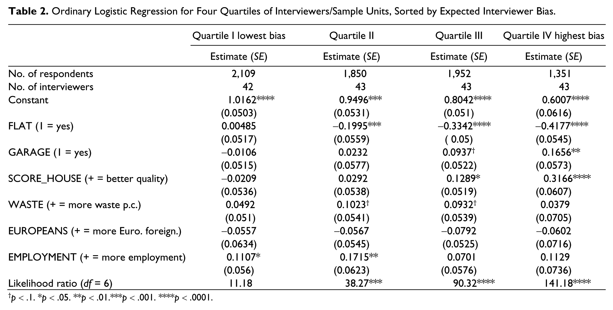
Part of the problem with the interviewer-specific estimates for the various quality indicators with regard to the obtained sample is their limited precision because of the relatively small number of sample units interviewers are assigned. Therefore, a more robust way of investigating the bias is used. Based on the distribution of maximal absolute bias, we divide the group of interviewers into four quartiles, so that the first group covers interviewers (and their assigned sample cases) with the smallest maximal absolute bias estimates, up to the fourth group, which comprises the 25% of interviewers with the largest bias. Ordinary logistic regressions are subsequently run for each of the four quartiles, modeling the response outcome based on all previously selected auxiliary variables. Table 2 shows the results.

Table 2.

Ordinary Logistic Regression for Four Quartiles of Interviewers/Sample Units, Sorted by Expected Interviewer Bias.

	Quartile I lowest bias	Quartile II	Quartile III	Quartile IV highest bias
	Estimate (SE)	Estimate (SE)	Estimate (SE)	Estimate (SE)
No. of respondents	2,109	1,850	1,952	1,351
No. of interviewers	42	43	43	43
Constant	1.0162****	0.9496***	0.8042****	0.6007****
	(0.0503)	(0.0531)	(0.051)	(0.0616)
FLAT (1 = yes)	0.00485	−0.1995***	−0.3342****	−0.4177****
	(0.0517)	(0.0559)	( 0.05)	(0.0545)
GARAGE (1 = yes)	−0.0106	0.0232	0.0937^†	0.1656**
	(0.0515)	(0.0577)	(0.0522)	(0.0573)
SCORE_HOUSE (+ = better quality)	−0.0209	0.0292	0.1289*	0.3166****
	(0.0536)	(0.0538)	(0.0519)	(0.0607)
WASTE (+ = more waste p.c.)	0.0492	0.1023^†	0.0932^†	0.0379
	(0.051)	(0.0541)	(0.0539)	(0.0705)
EUROPEANS (+ = more Euro. foreign.)	−0.0557	−0.0567	−0.0792	−0.0602
	(0.0634)	(0.0545)	(0.0525)	(0.0716)
EMPLOYMENT (+ = more employment)	0.1107*	0.1715**	0.0701	0.1129
	(0.056)	(0.0623)	(0.0576)	(0.0736)
Likelihood ratio (df = 6)	11.18	38.27***	90.32****	141.18****

†

p < .1. *p < .05. **p < .01.***p < .001. ****p < .0001.

It can be observed that the expected biases are strongly reflected in the estimates of the model in the four groups. First, the intercepts decrease from 1.02 in the first quartile (lowest bias) to 0.60 in the fourth quartile (highest bias), indicative of the expected response rates that should be highest in the first quartile, gradually decreasing until the last. Second, the magnitude and the p values of the slope estimators indicate that in the first quartile the predictive power of the auxiliary variables on the response behavior is very close to 0, whereas these parameter estimates in the fourth quartile are highly significant for SCORE_HOUSE and FLAT, and somewhat weaker for GARAGE. These findings are also reflected by the likelihood ratios of the four models. Therefore, the results in Table 2 show that low bias interviewers (quartile I) have the lowest bias, as they combine the highest response rates (as shown by the intercept) and no impact of the covariates (suggestive for low levels of contrast). Quartile IV has, as expected, the lowest intercept—indicating the lowest response rate—and the highest levels of contrast, as covariates have a strong effect on the response propensities.

Nevertheless, some validation of the results is desirable. First, we split the entire dataset randomly into two subsets of equal size. For each interviewer, half of the respective sample units are assigned to Subset A and the other half to Subset B. Then, the quality indicators for the obtained samples are calculated again per interviewer separately for A and B, after which the correlations for the response rates, contrasts, and biases are obtained between the two subsets.

The correlations are substantive and significant, but not convincingly high as Table 3 shows. This suggests that these results do not produce stable individual interviewer bias estimates and do not support an assessment of the interviewer force at the individual level. Larger datasets containing more observations per interviewer will be more suited for individual assessments. These could include labor-force surveys or other recurring surveys, often conducted by National Statistical Institutes and deploying a relatively permanent interviewer staff.

Table 3.

Cross-Validation for Interviewer-Specific Quality Indicators, 169 Interviewers.

Quality indicator	Correlation between Subsets A and B	p value
Response rate	.3781	<.0001
Maximal absolute contrast	.2782	.0003
Maximal absolute bias	.2334	.0023

Discussion

The quality assessment of a realized sample or a respondent set has been a response rate driven activity for a long time. However, as nonresponse is believed to be not completely at random, contrasts between respondents and nonrespondents, and particularly their associated bias estimates, have been more focused on recently. This shift from response rate oriented quality assessment toward more bias oriented assessment can be considered as an improvement in the assessment of nonresponse error in surveys. Nonetheless, such a shift imposes more fieldwork or administrative effort, as it requires relevant auxiliary information concerning all the sample cases. The restricted availability of powerful auxiliary variables is a particularly important obstacle to the assessment of nonresponse bias.

Although many survey researchers have estimated these biases at the sample level, a bias assessment may also be relevant at the interviewer level. Evidently, as interviewers are important contributors to the construction of the eventual respondent set, they may individually be responsible for systematic selection and bias creation. Therefore, we combine models to estimate nonresponse bias with models accommodating interviewer effects. Specifically, a binary response/nonresponse multilevel model is applied, allowing for both random intercepts and random slope effects at the interviewer level. Slope effects are applied to auxiliary variables, available for both respondents and nonrespondents. Given these intercept and slope parameters at the interviewer level, estimates of particular contrast and bias can be calculated for each interviewer.

From the empirical analysis on the Flemish Housing Survey, it is suggested that not all interviewers are equally prone to generate bias. For some interviewers, the slope parameters are very close to 0, indicating that they produce hardly any bias. For other interviewers, the impact of auxiliary variables is more substantial and therefore they produce more differences in the response propensities of the sample cases, increasing the risk of nonresponse bias. However, as the illustration indicates, to obtain accurate estimates of interviewer contrast and bias, random slope models may require more data than models containing only random intercepts. The Flemish Housing Survey is probably too small to support strong inferences about individual interviewer performances. Larger datasets, containing many sample cases per interviewer, are likely to be more appropriate for such interviewer evaluation purposes.

The method as presented in this article permits the monitoring of survey fieldwork, taking the interviewer as an important determinant of the quality of the obtained sample. It provides information about which interviewers perform better than others. One could consider offering interviewers a bonus based on their bias profile. This means that the bonus would not be based only on the realized response rate but also on the contrast between respondents and nonrespondents. The interviewer’s bias profile can also be an interesting starting point for more profound analysis of the fieldwork behavior and strategies of interviewers. The degree to which interviewers are identified as being prone to generate nonresponse bias may be related to, for example, their experience, workload (within the same or another survey project), and prioritization of particular sample cases. Of particular relevance are the differences in call patterns or doorstep interaction characteristics, which are probably more appropriate for some particular groups of respondents. This kind of information is useful to improve the part of the interviewer training that concerns contact and persuasion strategies. The message for interviewers is not only to increase response rates but also to avoid selectivity.

Footnotes

Appendix

Usually, multilevel models are applied to deal with interviewer effects. Based on such models, inferences can be made about the parameter estimates of the marginal model (fixed effects) and the variance of the intercepts (and slopes) at the second level. However, for this interviewer evaluation, the interviewer-specific parameters are of greater interest than the fixed parameters. These interviewer parameters may be obtained by adding the interviewer-specific deviation $\hat{u}$ to the fixed parameter $\hat{γ}$ . However, what are termed the empirical Bayes (EB) estimates are probably biased due to parameter shrinkage (see, for example, Hox, 2002; Raudenbush & Bryk, 2002; Snijder & Bosker, 1999) or partial pooling (Gelman & Hill, 2007). Particularly, interviewers who have been assigned to a small group of sample cases may therefore have intercept and slope parameters that are shrunk toward the fixed parameter estimates of the marginal model. As a result, the obtained interviewer bias estimates are too small.

Alternatively, a (logistic) regression model can be run for each interviewer separately. However, because of the small number of assigned cases per interviewer, the intercept and slope parameter may become unbiased and also very unstable, whereas the EB estimates may be relatively stable (small standard errors), but biased toward the marginal model estimates. Ideally, a great deal of data would be available per interviewer, so that the EB estimates and the one-model-per-interviewer estimates converge. This could be possible by considering the fieldwork results of interviewers over a long period of time, possibly comprising multiple survey projects. Unfortunately, the data used in the current article only consider one survey project, where the workload per interviewer was relatively limited. Therefore, the EB estimates are converted into measurements that are less biased toward the marginal model, at the expense of less stability (greater standard errors).

With regard to the intercepts, the EB estimate is a weighted average of the estimated fixed intercept parameter ${\hat{γ}}_{00}$ and ${\hat{β}}_{0 j}$ , the intercept estimated from a (logistic) regression for interviewer j alone:

{\hat{β}}_{0 j}^{EB} = λ_{j} \hat{β} + (1 - λ_{j}) {\hat{γ}}_{00},

where the weight $λ_{j}$ is the reliability of ${\hat{β}}_{0 j}$ and $λ_{j}$ is provided by the equation:

λ_{j} = \frac{σ_{0}^{2}}{σ_{0}^{2} + \frac{σ_{e}^{2}}{n_{j}}} .

When an interviewer has been assigned to a large group of sample cases, the reliability will be closer to 1, so that the EB estimate will only be modestly pushed toward the marginal mean. This explains why the EB estimates are biased. However, because they also rely on the marginal estimates, they will have greater precision.

It is obvious that we do not want to use the biased EB estimates, but prefer the less precise estimates that would result from performing as many (logistic) regressions as there are interviewers. However, ordinary (logistic) regression does not allow for the inclusion of area variables that have practically no variation at the interviewer level, but seems necessary to separate interviewer effects from area effects. Therefore, we choose to derive the interviewer parameters from the multilevel analysis. As we know that

{\hat{β}}_{0 j}^{EB} = λ_{j} {\hat{β}}_{0 j} + (1 - λ_{j}) {\hat{γ}}_{00},

we specify that

\begin{array}{l} \frac{{\hat{β}}_{0 j} = {\hat{β}}_{0 j}^{EB} - (1 - λ_{j}) {\hat{γ}}_{00}}{λ_{j}} \\ \frac{= {\hat{β}}_{0 j}^{EB} - {\hat{γ}}_{00} + λ_{j} {\hat{γ}}_{00}}{λ_{j}} . \\ = \frac{{\hat{u}}_{j} + λ_{j} {\hat{γ}}_{00}}{λ_{j}} \\ = \frac{{\hat{u}}_{j}}{λ_{j}} + {\hat{γ}}_{00} \end{array}

Deriving the ${\hat{β}}_{0 j}$ s from the EB estimates also seems to produce more robust estimates than in the case of ordinary (logistic) regression.

A final remark relates to the estimation of the interviewer-specific parameters concerning the response variable that is binary instead of normally distributed. Specifically, the weight factor $λ_{j}$ that determines the reliability of ${\hat{β}}_{0 j}$ should be re-specified into

λ_{j} = \frac{τ_{0}^{2}}{τ_{0}^{2} + \frac{π^{2}}{3 n_{j}}},

as the standard deviation of the residuals in logistic multilevel regression is believed to be $\sqrt{π^{2} / 3} = 1.81 .$

In this regard, consider a situation where J = 1, 2, …, 160 interviewers are involved, and all variables Y should be regressed by a variable X, allowing for both random interviewer intercepts and slopes with respect to X or

Y_{i j} = γ_{00} + u_{0 j} + γ_{10} x + u_{1 j} x + ε_{i j} .

The fixed effects are γ₀₀ = 1 and γ₁₀ = .5. The variance of the random intercepts equals $σ_{μ_{0}}^{2}$ = 1 and the variance of the random slopes equals $σ_{μ_{1}}^{2}$ = .25. The first 40 interviewers have been assigned to only 20 sample cases, the second quartile of 40 interviewers has been assigned to 40 sample cases, the third quartile to 60 cases, and the fourth quartile of 40 interviewers have been assigned to 80 cases.

All individual interviewer parameters for intercepts and slopes are known, accommodating a simulation study where 250 samples are drawn from the situation as presented above. This means that for each interviewer the true parameters $(γ_{00} + u_{0 j} and γ_{10} + u_{1 j})$ can be compared with the means of their 250 sampled counterparts, both with respect to the original EB estimates and the new estimates that try to undo the shrinkage effect. Table A1 presents the simulation results.

It is clear from the table that the bias is reduced when considering the new estimates as compared with the EB estimates. Although the bias is reduced, the new estimates are less stable, as their variance is larger than the EB estimates.

Nevertheless, it should be emphasized that a larger dataset, containing more individual interviewer records, is preferable to obtain unbiased and presumably more stable interviewer estimates for both intercepts and slopes.

Declaration of Conflicting Interests

The author(s) declared no potential conflicts of interest with respect to the research, authorship, and/or publication of this article.

Funding

The author(s) received no financial support for the research and/or authorship of this article.

Author Biographies

Geert Loosveldt is Professor at the Centre for Sociological Research at the KU Leuven. He teaches courses about Social Statistics and Survey Research Methodology. His research focuses on evaluation of survey data quality with special interest in the evaluation of interviewer effects and the causes and impact of non-response error.

Koen Beullens (PhD) is a senior researcher at the Centre for Sociological Research at the KU Leuven. His main research topics are nonresponse error and interviewer variance in survey research.

References

Bethlehem

(2009). Applied survey methods: A statistical perspective. Hoboken, NJ: Wiley.

Bethlehem

Cobben

Schouten

(2011). Handbook of nonresponse in household surveys. Hoboken, NJ: Wiley.

Biemer

Lyberg

(2003). Introduction to survey quality. New York, NY: Wiley.

Campanelli

O’Muircheartaigh

(1999). Interviewers, interviewer continuity, and panel survey nonresponse. Quality & Quantity, 33, 59-76.

Dalenius

(1983). Some reflections on the problem of missing data. In Madow

W. G.

Olkin

(Eds.), Incomplete data in sample surveys. Vol. 3: Proceedings of a Symposium (pp. 411-413). New York, NY: Academic Press.

Durrant

Groves

R. M.

Staetsky

Steele

(2010). Effects of interviewer attitudes and behaviors on refusal in household surveys. Public Opinion Quarterly, 74, 1-36.

Durrant

Steele

(2009). Multilevel modelling of refusal and non-contact in household surveys: Evidence from six UK government surveys. Journal of the Royal Statistical Society: Series A, 172, 361-381.

Gelman

Hill

(2007). Data analysis using regression and multilevel/hierarchical models. Cambridge, UK: Cambridge University Press.

Groves

(2006). Nonresponse rates and nonresponse bias in household surveys. Public Opinion Quarterly, 70, 646-675.

10.

Groves

Cialdini

Couper

(1992). Understanding the decision to participate in a survey. Public Opinion Quarterly, 56, 475-495.

11.

Groves

Couper

(1998). Nonresponse in household interview surveys. New York, NY: Wiley.

12.

Groves

Peytcheva

(2008). The impact of nonresponse rates on nonresponse bias. A meta-analysis. Public Opinion Quarterly, 72, 167-189.

13.

Hox

(2002). Multilevel analysis: Techniques and applications. Mahwah, NJ: Lawrence Erlbaum.

14.

Little

(1986). Survey nonresponse adjustments for estimates of means. International Statistical Review, 54, 39-157.

15.

Little

(1988). Missing-data adjustments in large surveys. Journal of Business & Economic Statistics, 6, 287-296.

16.

O’Muircheartaigh

Campanelli

(1999). A multilevel exploration of the role of interviewers in survey non-response. Journal of the Royal Statistical Society: Series A, 3, 437-446.

17.

Peytchev

Riley

Rosen

Murphy

Lindblad

(2010). Reduction of nonresponse bias in surveys through case prioritization. Survey Research Methods, 4(1), 21-29.

18.

Pickery

Loosveldt

(2002). A multilevel multinomial analysis of interviewer effects on various components of unit nonresponse. Quality & Quantity, 36, 427-437.

19.

Raudenbush

Bryk

(2002). Hierarchical linear models: Applications and data analysis methods. Thousand Oaks, CA: Sage.

20.

Schnell

Kreuter

(2005). Separating interviewer and sampling-point effects. Journal of Official Statistics, 21, 389-410.

21.

Schouten

Cobben

Bethlehem

(2009). Indicators for the representativeness of survey response. Survey Methodology, 35, 101-113.

22.

Shlomo

Skinner

Schouten

Bethlehem

Zhang

(2009). Statistical properties of R-indicators (RISQ deliverable 2.1). Available at www.r-indicator.eu.

23.

Snijder

Bosker

(1999). Multilevel analysis: An introduction to basic and advanced multilevel modelling. London, England: Sage.

24.

West

B. T.

Kreuter

Jaenichen

(2013). Interviewer effects in face-to-face surveys: A function of sampling, measurement error or nonresponse? Journal of Official Statistics, 29, 277-297.

25.

West

B. T.

Olson

(2010). How much of interviewer variance is really nonresponse error variance? Public Opinion Quarterly, 74, 1004-1026.

A Procedure to Assess Interviewer Effects on Nonresponse Bias

Abstract

Keywords

Introduction

Review of Sample Quality Indicators Based on Estimated Response Propensities

Multilevel Models and the Assessment of Interviewer Effects on Nonresponse: A Random Slope Extension

Illustration: Flemish Housing Survey 2005-2006

Data

Results of a Multilevel Model With Random Intercept and Random Slopes

Interviewer-Specific Quality Indicators for the Flemish Housing Survey

Validation of the Indicators at Interviewer Level

Discussion

Footnotes

Appendix

Declaration of Conflicting Interests

Funding

Author Biographies

References