Sage Journals: Discover world-class research

Abstract

This article discusses issues of scales in measuring attitude, demonstrates how a metric scale can be generated based on three main features, and presents results from a repeated measurement survey to verify the generated scale. The design of the generated metric scale is introduced and named Ruler and Option (RO). The population for repeated measurement survey was 1,870 bachelor students from a public university. Two sets of questionnaire (identical items), one with 7-point Likert scale and another with RO scale, were distributed to a sample of 595 bachelor students chosen using stratified random sampling method. Data were analyzed descriptively using SPSS version 20 and structural equation modeling using AMOS version 21. Results showed that data from RO scale performed better than data from 7-point Likert scale in terms of number of items per construct, factor loadings, squared multiple correlations, higher ratio of degrees of freedom to number of parameters, and higher reliability coefficients. In terms of validity coefficients, measurement models from both data sets attained almost the same level of discriminant and construct validity. Further studies are recommended to elicit the strength and weakness of RO scale to identify the situations where it is most suitable.

Keywords

interval measurement level Likert scale measure attitude RO scale measurement theories

The phenomena of treating ordinal data as intervals have been criticized by many scholars (Chimi & Russell, 2009; Grace, 2008; Henson, Hull, & Williams, 2010; Jamieson, 2004; Knapp, 1990), especially by those who uphold the philosophy of numbers and number operations. Harwell and Gatti (2001) scoured through three educational journals, American Educational Research Journal, Sociology of Education, and Journal of Educational Psychology, and noted that 73% of the dependent variables in articles from 1993 to 1997 appeared to be ordinals but were treated as intervals, thus using analyses that lead to queries in validity of inference. According to Agresti (2002) and Clogg and Shihadeh (1994), non-parametric statistical analyses should be applied to ordinal variables whereas parametric analyses should be applied to variables that achieve at least interval level of measurement (Davison & Sharma, 1988). Researchers such as Fadiya (2013), Amah (2013), Wilson, Wainwright, Stehly, Stoltzfus, and Hoff (2013), and Kornfeld (2013) had used 5-point Likert scale in their studies and treated data as ordinals by applying non-parametric analyses such as ordinal logistic regression, Mann-Whitney, and chi-square tests. On the other hand, Sarafidou (2013), Jain (2013), Razzaque (2013), and Zaimah et al. (2013) had also used 5-point Likert scale in their research but treated data as intervals by applying parametric analyses such as mean, t-test, analysis of variance (ANOVA), regression, and factor analysis. This is an example of the phenomena of treating ordinals as intervals described by Harwell and Gatti (2001) and other researchers such as Knapp (1990), Jamieson (2004), Grace (2008), Chimi and Russell (2009), and Henson et al. (2010).

Two root causes have been identified as the reason researchers persist on treating ordinals numerically. The first root cause is the desire to quantify the intangibles and second, the absence of a globally accepted measuring scale that can be used to translate intangibles into numbers. Variables such as attitude, opinion, and feelings are considered as intangibles in the sense that they cannot be seen or touched, only experienced and felt. Classified as qualitative variables, they only qualify for ordinal measurement level. However, with the advancement of digital technology, men are becoming more and more a digitalized society so much so that they are not satisfied with subjective judgments; instead, they want to quantify or translate their expression of feelings, opinion, and attitude in terms of numbers. Question arises whether it is correct to perceive these intangibles as quantitative magnitudes. The authors are of the opinion that there is nothing wrong in doing so; in fact, numbers have the objective characteristic that indirectly implies independence and non-biasness. To illustrate the independence and non-biasness of numbers, let’s take an everyday example of someone suddenly losing weight and always feeling tired. A suggestion that he or she might be diabetic would quickly be brushed off as the condition is due to the hot weather or working too hard lately. However, a blood sugar level score of 17 moles per gram would confirm the gravity of his or her diabetes. The big difference (an expression in terms of numbers) from the reading of a normal non-diabetic person of 5.5 moles per gram is automatically comprehended compared with the subjective judgment by a friend. Subjective judgment by a friend may be dependent on the friend’s knowledge or experience thus prone to be biased toward a certain suggestion. Instead, by using a certain procedure to express the person’s condition in terms of numbers provides an independent, non-bias judgment, and usually readily accepted by the person.

Next question arises whether it is possible to convert these intangibles into quantitative magnitudes. The authors say yes, with a correct and suitable scale it is possible to do so. This provokes the next obvious question: “Is there such a scale.” To measure variables such as feelings, attitude, and opinion, researchers such as Gordon, Mahabee-Gittens, Andrews, Christiansen, and Byron (2013) and Geramian, Mashayekhi, and Ninggal (2012) used measurement scales that consist of a limited number of categories with vague zero point and vague unit of measurement. The categories are normally ordered but the distances between them are still unknown. A set of scores or numbers are assigned to the categories to enable respondents to express their opinion about an issue in terms of both strength and direction. This scale is known as Likert scale (Munshi, 1990). The actual number of categories is not an important issue. It is up to individual researcher to choose the number of categories according to his or her preference and expert knowledge, for example, Gordon et al. (2013) and Geramian et al. (2012) used 5-point Likert scale to collect their data.

So far social scientists have not reached to a consensus of a scale that could measure or interpret intangibles as quantitative magnitudes. The absence of a globally acceptable scale is identified as the second root cause. This root cause sparks an ongoing debate between measurement theorists regarding measurement of intangible variables in social sciences. The fuel is none other than one party is adamantly insisting that whatever variable is represented numerically on a rating scale should have relationships between its values isomorphic to the relationships between the numbers (Albaum, 1997; Harwell & Gatti, 2001; Knapp, 1990; Michell, 1997; Trendler, 2009). Thus, a Likert scale data should be considered ordinal. While the other party insists that no practical harm is done if data from such rating scales can be considered as interval and as such be treated as numerical (Dolnicar & Grun, 2007; Kemp & Grace, 2010). Agresti (2002) considered an ordinal variable that is assigned a set of scores to be quantitative in the way that each level has its own magnitude and can be compared with other levels in terms of size. This inherent quantitative aspect makes an interval variable different from a nominal variable. However, Meulman (1998) was of the opinion that a rating scale that has an uncertainty or vagueness of zero point and measurement unit may have a systematic component and therefore may not be just a matter of measurement error. Norman (2010) was of the opinion that parametric statistics are robust enough to be applied to ordinal data from Likert scales. In his counter reply to Trendler’s (2009) argument, Markus and Borsboom (2011) argued that measurement in psychology cannot be assumed equivalent to measurement in the natural sciences such as physics and as such, currently existing tests cannot be considered as measurements stoutly anticipated by Trendler (2009) and Michell (1997, 1999). Further investigations along this line to prove whether or not psychological measurement is possible would surely enlighten and advance the field.

The objective of this article is twofold: (a) to demonstrate the generation of a scale that is continuous (metric) and objective (numerical), has a measurement unit and meaningful zero point, complies with the requirement of measurement theories, and can be easily administered and responded, and (b) to verify the scale by comparing performance of data collected using the generated scale with performance of data collected using a well-known scale such as Likert scale. By developing the scale, the authors expect to show that intangible variables such as feelings, attitude, and opinion can be correctly expressed in terms of numbers and hopefully this scale can be accepted by both parties described in the above paragraph as a possible solution to measuring these intangibles.

Before going deeper into the discussion of developing the scale, a review of the measurement theories, definitions of type of variables, and measurement scales already available in social science would provide a better understanding of the whole phenomena of treating ordinal data as intervals.

Review of Literatures

Measurement Theories

The three main theories on measurement are classical, representational, and operational measurement theories (Hand, 1996; Presser & Schuman, 1989). One of the earliest definitions of measurement was given by Campbell in 1920 (as cited in Hand 1996, p. 446), who described measurement as the assignment of numerals to represent the properties of objects, where the objects satisfy (a) an order relationship and (b) a physical process of addition (concatenation). In the same tone, Stevens (1946) coined the idea of measurement as assigning numbers to items or events according to rule (Matheson, 2008; Michell, 1999). This is known as representational measurement theory, which is the dominant current measurement idea. Suppes and Zinnes (1963) discussed isomorphism between arithmetical structures (order and concatenation) and structures of values of variables. This means that certain aspects of the number arithmetic have the same structure as the empirical situation being explored. The importance of finding such an isomorphism of structures is that familiar computational methods, applied to the arithmetical structure, may be used to infer facts about the isomorphic empirical structure. To illustrate, let’s say we have a few bricks piled up to be weighed one by one. If the weight which is the number assigned to a brick is bigger than the number assigned to another brick, then we can conclude that the first brick is heavier than the other. Thus, a relationship among the numbers (greater than) corresponds to a relationship among the bricks (heavier than). If we weigh all the bricks together, then the number assigned to the total weight will be equal to the total of individual number. Another relationship among the numbers (addition) correlates to the relationship among the bricks (total or concatenated weight). According to representational measurement theory, these relationships must be proven for the measurements to be valid. Marcus-Roberts and Roberts (1987) wrote that Stevens (1946, 1951, 1959) offered a solution to the representational debate in social sciences when he coined his theory of the four possible types of measurement levels (nominal, ordinal, interval, and ratio). Different statistical analyses are allowed for different measurement scale or level. However, a gray area still covers the interval level for certain scientist considers it ordinal while others regarded it as quantitative (Kemp & Grace, 2010).

The operational measurement theory concentrates on the operations or procedures used to measure a variable. It is based on the idea that a concept is not understood until there is a method to measure it (Chang, 2009). In 1927, the American physicist P.W. Bridgman, who coined the theorem, stated that “we mean by any concept nothing more than a set of operations” (as cited in Chang, 2009). This means that a variable is defined by its measuring procedure. Hence, to have a useful measurement of a variable, the numerical assignment procedure has to be well-defined. Accordingly, a questionnaire that requires a respondent to rate items must provide clearly defined procedure (operation) on how to arrive to a rating. This is essential because when everybody uses the same conventions to discuss some phenomenon, then useful discussions can take place (Hand, 1996). Without any specific procedure to follow, respondents will have their own varied procedures in which to produce a rating. This is why problems arise in psychological measurement because measuring procedures are not operationally well-defined. Different researchers may use the same values for variables that may be delicately different.

The classical measurement theory, which contrasted with the representational and operational theories, was first described by Michell (1986). Michell called it classical because he claimed that traces of the theory were found in the works of Aristotle and Euclid. This theory only refers to quantitative variables because according to the theory, measurement seeks to find out “how much” of a trait an object has. For example, let’s consider the statement, “the height of a cupboard is 250 centimeters.” In this case, height is the trait and centimeter is the unit of the magnitude. The trait height must have the properties that satisfy ordinal and additional relationships, not the object cupboard. The behavior of the object may or may not resemble the quantitative nature of the related trait. In other words, measurement is concerned with discovery of existing relationship among the quantitative magnitude of the trait. By classical definition, measurement is the evaluation of ratios of quantities (Michell, 1999). In principle, quantity and measurement are equally defined. Prior to measuring an attribute, Michell (1997) urged scientists to first prove that a variable is quantitative or having quantitative structure, then devise methods to measure its magnitude. He strongly argued that if a scientist only allocates numbers to things according to some rule while ignoring the fact that the measurability of the thing assumes that it possesses an additive structure, then the scientist would be inclined to believe that the creation of suitable numerical assignments alone generates scientific measurement. This creates an unfortunate phenomenon that he called “systemically sustained blind spot” in quantitative psychology.

The process of interpreting research results from data analyses has to incorporate measurement theories, measurement level, and statistical analyses. Without incorporating these three factors, researchers may interpret results by making meaningless statements (Marcus-Roberts & Roberts, 1987). The scale used must virtually conform to measurement theories to warrant quantitative analyses. On the other hand, if the scale does not conform to measurement theories, then researchers have to determine the data measurement level to ensure correct application of statistical analyses. In this way, results obtained are more valid enabling better deduction. Sarle (1997) pointed out that to make inferences about reality, it is necessary to consider both statistical theory and measurement theory. Statistical theory provides connection between inference and data while measurement theory, between data and reality. Jamieson (2004) suggested that to raise the research quality, authors must address issues on measurement level and parametric statistics at the research design stage. Researchers should not be hasty in deciding the choice of scale of measurement. Jamieson considered the legitimacy of assuming an interval scale for Likert type categories as a significant issue. This is because a poor scale may provide inadequate information especially when doing predictive modeling (Velleman & Wilkinson, 1993).

Discrete, Continuous, and Ordinal Variables

To be able to differentiate between continuous, discrete, and ordinal variables, readers must have an understanding of the definition as well as the procedure(s) involved in obtaining the variables. According to Mann (2001), a discrete variable assumes values that are obtained from counting, for example, number of houses in a certain block while continuous variables are obtained by measuring and thus, assumes any value contained in an interval, for example, the height of a person. On the other hand, ordinal variables are obtained by ranking. Therefore, discrete and continuous variables are quantitative whereas ordinal variables are qualitative. Discrete variables give rise to discrete probability distributions such as Binomial and Poisson distributions, whereas continuous variables give rise to continuous probability distributions such as the Exponential distribution and the prominent Normal distribution. So we can see the strong relationship between continuous variables and the Normal distribution, which is one of the assumptions to be fulfilled in parametric statistical analyses.

Now let us elaborate the definition of continuous variables further by explaining the procedure involved in obtaining the variables. To obtain the values of a discrete variable, all one has to do is to count; hence, the operational procedure is counting. That is why the exact values of a discrete variable can be obtained. In contrast, values of a continuous variable are obtained using a measuring tool or scale that implies the existence of a more elaborate operational procedure that must be clearly defined as the basis for measurement. Because of the dependence on a measuring instrument, values obtained will be subjected to measurement errors, not exact, and fall within an interval that consists of infinite points. Accuracy of the values obtained depends on the accuracy of the instrument. Let’s go back to the previous example of a continuous variable, that is, the height of a person. To obtain the height of a person, we need a measuring tool such as a ruler. The ruler is put behind the person to be measured and the researcher reads off the mark on the ruler that corresponds to the height of the person. Because we accept the existence of measurement errors, we usually take several measurements using the same operational procedure and calculate the average value. This average value will be taken as the representation of the height of the person. Another way of getting several values of the height of a person is to gather a number of people to conduct the same operational procedure with the same measurement tool. Using both ways, not all the values of the height obtained will be exactly equal; in fact, the values will be between the lowest and the highest value obtained for the height of the person being measured. This is what is meant by continuous variables assume any value contained in an interval. Some of the values obtained may occur more frequently than the others so that we can generate different probabilities for different values called the probability distribution. Because the interval contains infinite points, these probabilities will give rise to a continuous probability distribution of the height of the person. If sample of persons’ height to be measured is big enough, the continuous probability distribution may attain the characteristics of a Normal distribution.

Measurement Scales in Social Science

Several scales have been devised by various researchers to measure intangible variables such as feelings, attitude, and opinion. They are semantic differential scale, Stapel scale, Thurstone differential scale, and direct rating scales (Albaum, 1997). These scales are also known as itemized rating scales (Russell, 2010).

Semantic differentials are among the most widely used scales to measure attitude (Heise, 1969). A semantic differential scale usually consists of a series of 7-point or 5-point bipolar rating scales. Each descriptive item contains two adjectives, opposite in meaning, such as “good” and “bad,” “modern” and “old fashioned,” on either end of the scale. Participants are asked to identify where on the scale usually from 1 to 7 or 1 to 5, they feel the object fits in relation to the two adjectives. Scores with higher numbers reflect more positive evaluations. The scores are then summed or averaged to provide an overall score (Garland, 1990).

Stapel scale is a slight modification of semantic differential scale (Hawkins, Albaum, & Best, 1974).It is easier to conduct and administer especially in situations when it is difficult to create pairs of bipolar adjectives. The scale consists of a single adjective in the middle, a unipolar, numbered from −3 to +3(as an example), without a 0 point. The higher the positive score implies the better the adjective describes the issue or object concerned. Data collected using Stapel scale can be analyzed in the same way as semantic differential data (Russell, 2010).

The Thurstone scale is a technique that takes into account the strength of individual item in computing the attitude score. There are three different scales developed by Thurstone (Fabrigar & Paik, 2013): equal appearing intervals, the method of paired comparisons, and the method of successive intervals. Among the three scales, an equal appearing interval scale is the most popular and thus described in this paragraph. First of all, a number of statements or indicators of an attitude variable will be generated. Then judges or experts will be asked to rank the statements by giving numbers, for example, from 1 to 11, where 1 indicates the weakest indicator of the variable and 11 indicates the strongest indicator of the variable. The ranks by the experts will be averaged and assigned to each indicator as weights. If an indicator has a high degree of variability (little consensus) in rankings by the judges, then the indicator will be discarded. Finally, a set of statements together with their strength (weights) in indicating an attitude is generated. During a survey, respondents will be asked to tick or check which statement(s) they think represent their attitude toward the variable. For each respondent, the weights of the checked statements will be summed and divided by the number of statements being checked, giving a score that will represent the respondent’s attitude toward the variable (Babbie, 2001).

A rating scale is a set of categories that are assigned numerical values designed to elicit information (by self-reporting) about a quantitative or a qualitative attribute. For example, to measure “influence,” suitable categories are “not at all influential” (assigned number 1), “slightly influential” (assigned number 2), “somewhat influential” (assigned number 3), “very influential” (assigned number 4), and “extremely influential” (assigned number 5; Vagias, 2006). The most common rating scale is called the Likert scale developed by Rinsis Likert in 1932 (Munshi, 1990). The scale that can be easily administered and responded was intended to be a summated scale, which was then assumed to have interval properties. However, the individual scale is not assumed to be interval even though more often than not it is treated as such (Albaum, 1997). According to Boone and Boone (2012), data from individual Likert item are considered as ordinals and can be analyzed using non-parametric methods such as mode or median for central tendency, frequencies for variability, and chi-square test, Kendall Tau B, and Kendall Tau C for measuring association. Whereas as a summated scale, data from Likert scale are considered as intervals and can be analyzed using parametric methods such as mean for central tendency; standard deviations for variability; Pearson’s r, t-test, ANOVA, and regression procedures (Boone & Boone, 2012). Nowadays, Likert scale is omnipresent in many fields of research especially when measuring a value such as belief, opinion, or affect, which cannot be precisely measured by respondents. Take for example, articles in the Journal of Extension; at least 21 articles published in 2010 and at least 12 articles published in 2011 used Likert scale in their study (Boone & Boone, 2012). It is also popular in measuring a value that is naturally sensitive such that a respondent would not be able to answer except by choosing from a large range of categories (Chimi & Russell, 2009).

All the scales described above use numbers to reflect the direction of strength of an unobservable or intangible variable such as feelings, attitude, and opinion toward a certain issue or given object. Data collected from these scales are in the form of numbers and analyzed quantitatively (Babbie, 2001; Boone & Boone, 2012;; Russell, 2010,Hawkins et. al 1974). However, if we refer to the definition of discrete and continuous variables, these data are actually not quantitative; in fact, they are coded values that represent the strength or ranks a respondent chose to mark on the scale. Hence, the application of quantitative statistical analyses is inappropriate. Likewise, even though Likert summated scale can be considered as interval (Boone & Boone, 2012), we have yet to find the correct explanation to justify the transformation of a group of ordinal data (individual Likert item) into interval data. Current methods to determine latent variables such as factor analysis and covariance based structural equation modeling (CB-SEM) do not explain the transformation but assume that data are normal and linearly related (Hair, Black, Babin, & Anderson, 2010).

Shortcomings of Likert Scale

Respondents using Likert scale tend to rate the middle value, which is defined as a neutral position, as neither agree nor disagree, excluding the categories “no knowledge” and “no opinion” (Albaum, 1997). The problem with this is that the researcher wouldn’t know whether data would represent genuine neutral stand, uncaring attitude, or whether the respondent actually does not have any knowledge on the subject of interest. The problem of trying to categorize a respondent’s attitude is intensified when the respondent rated the middle value for all the questions. In this situation, researchers should think whether all the responses can be considered to be valid responses. The semantic meanings and positions of the scale labels influence respondents’ ratings (Wildt & Mazis, 1978). The various choices of words may point to various levels of feelings, attitude, or understanding for different people. Thus, different respondents might think or feel differently but rated the same value. The number of categories assigned to each item in the scale may not be appropriate (Ferrando, 2003; Munshi, 1990). Based on his findings, Ferrando (2003) suggested that the number of points effectively used by respondents depended on the type of scale (either graphical or numerical), respondents’ motivational and cognitive characteristics, type of variable measured, type of administration (paper and pencil or Internet), and interactions among these factors. Scherpenzeel and Saris (1997) believed that there is no optimal number of response alternatives. The distances between each category are not equal (Ferrando, 2003; Munshi, 1990). This fact coupled with absence of meaningful zero point in a Likert scale aggravates the use of arithmetic mean to represent the intangible variables. Jamieson (2004) confirmed that the categories are ranked order and distance between the intervals cannot be assumed equal. Thus, the mean and standard deviation are not appropriate even though it is common practice among authors to describe their data using these statistics. Likert-type and ordinal items are coarse and inexact, and information is lost because data are not sufficiently discriminating (Aguinis, Pierce, & Culpepper, 2009). The scale lacks measurement unit and does not conform to the requirements of any of the three measurement theories to warrant it quantitative.

Approaches Offered by Researchers

Several researchers (Granberg-Rademacker, 2010; Harwell & Gatti, 2001; Hsu, Chang, & Hung, 2007; Wu, 2007) have approached the problem by rescaling Likert data using several methods in mathematical modeling. Others developed a different type of scale using continuous line segments called “Continuous Response Scale” or “Visual Analogue Scales” (Aitken, 1969; Cella & Perry, 1986; Ferrando, 2003; Lerdal, Kottorp, Gay, & Lee, 2013; Munshi, 1990; Pfennings, Cohen, & van der Ploeg, 1995; Puzziawati Ab Ghani & Abdul Aziz, 2005).

Mathematical modeling

Mathematically proficient researchers opted for mathematical modeling to rescale ordinals into continuous intervals using methods such as Markov Chain Monte Carlo, Snell method, Fuzzy Logic, and Item Response Theory (IRT; Granberg-Rademacker, 2010; Harwell & Gatti, 2001; Hsu et al., 2007; Wu, 2007). Wu (2007) applied Snell’s scaling procedure to convert data from 4-point and 6-point Likert scale to numerical scores. Wu introduced concepts and computation procedure for determining the numerical scores and stated that there is a linear complexity in terms of computer time and space requirements. Wu also found that results from analysis of Snell’s data and Likert data are very much the same. Bharadwaj (2007) used fuzzy logic procedure to rescale data obtained from Likert scale in the Functional Independence Measure (FIM) model into continuous data. Bharadwaj applied parametric tests on the rescaled data and Likert data and found that results were similar. Harwell and Gatti (2001) preferred to use IRT to rescale ordinal data into intervals because they were of the opinion that IRT produces interval-scale data, satisfying measurement-based arguments. However, Harwell and Gatti emphasized that IRT models are complex and come with rigorous assumptions that must be satisfied for the models to be of value. Harwell and Gatti rescaled 30 dichotomously scored items using IRT (Rasch model) and found that 10 of the items showed inadequate fit, which may be due to a failure to model item discrimination and/or the likelihood of guessing. Harwell and Gatti also used Samejima graded response model to rescale scores from 5-point rating scale into intervals and found that the model did not adequately fit the data.

All of the mathematical modeling methods started with data collected using Likert scale or other ordinal scales, which were then manipulated into interval data. Apart from the complex procedures, there is the question of how accurate the rescaled data do represent the actual data.

Continuous line segments

Many researchers had come up with continuous line segments of different lengths and labels (Aitken, 1969; Cella & Perry, 1986; Ferrando, 2003; Munshi, 1990; Pfennings et al., 1995; Puzziawati Ab Ghani & Abdul Aziz, 2005). Chimi and Russell (2009) recommended a continuous scale consisting of line segments presented on a full screen graphical user interface (GUI). Although the continuous line segments offered overcome the coarseness of Likert scale by providing infinite points as choices, there are still apparent weaknesses. The absence of clearly defined operational procedure for respondents to follow to obtain a score still classifies the scale as ordinal level. This is because even though the mark on a line between 0 and 100 may produce real decimal numbers, they are actually coded values or ranks and can be replaced by other coded values, for example, from a line marked 1 to 10 or another line marked 100 to 1,000. The number 0 does not imply ‘nothing’. The middle point effect, absence of measurement unit, and subjective use of semantics are other weaknesses. Furthermore, the process of measuring the distance between the beginning of the line and the point (Dolnicar & Grun, 2007) where respondents put a mark can be quite a hassle and not very “researcher friendly.” The use of GUI is computer dependent and although could be incorporated with automated system of data processing, still has to face the problem of low response rate in the case of uncontrolled situation of data collection procedure.

Hence, a scale that is continuous (metric) and objective (numerical), has a measurement unit and zero point, complies with the requirement of measurement theories, and can be easily administered and responded would be an alternative longed for.

Scales for Measuring Attitude Should Be Continuous

Why should the scale be continuous? Are human thinking and feeling continuous or categorical? Now, let us look at the way human beings think and feel. Because we are trying to measure these variables, we have to specify whether human “thinking and feeling” are continuous or categorical. To find out, let’s observe the processes involved in thinking. What is thinking? Thinking involves analyzing, examining, and sorting out information, and figuring ideas, feelings, or attitudes. All these processes are completed in split seconds in the mind to enable a person to perform an action quickly in times of emergencies. In other times when more information has to be collected before a decision is made and action taken, the process of thinking will consume an interval of time. Diller (1975) cited Polanyi’s argument that there is a “tacit component” to our knowledge. He says, “We can know more than we can tell and we can tell nothing without relying on our awareness of things we may not be able to tell” (p. 55). Our emotional and physical conditions influence the ways we think (Pennebaker et al., 1990). The relationship between emotions and emotional states can be calculated using Fuzzy functions (Ayesh, 2004), which is a type of mathematical logic where the actual or true value presumes a continuum of values between 0 and 1. “Emotional states are used to estimate action emotional triggers” (p. 875). The use of fuzzy functions to estimate human emotional states, which in turn can be used to estimate human actions, shows that human thinking and feelings are in fact continuous variables. Human behavior in general is in fact very hard to be categorized into permanent specific categories. Aitken (1969) described feelings as states of the person that incorporate moods and sensations. No exact words may be able to accurately describe the subjective personal experience. The lack of suitable quantitative terms in common speech limits the amount of information that can be transferred. Because no one has yet shown that feelings can be broken down into or made up of minute discrete amount of feelings (as in the case of mass and light), this phenomenon can still be considered as continuous and thus most appropriately entertained with continuous metric scale.

Why not just opt for non-parametric methods? Ratio and interval level of measurement are considered to be typical data for the application of parametric methods, while non-parametric methods are typically applied to ordinal and nominal data. If non-parametric methods are opted for Likert data (individual and summated), then quantitative assumptions of the data will not be important anymore. Hence, the hustle and bustle of the ambiguity status of Likert scale will naturally subside and the scale will be fully considered as ordinal!

Usability of Rating Scales

One important aspect of measuring is the utility of the scale that implies instructions on how to use the scale are simple and easily understood (Stone & Stenner, 2012). Another aspect is portability, which means useful in all locations; in the case of a rating scale, the author interprets it to mean applicable to many researches. Dolnicar and Grun (2007) observed that user-friendliness of scale formats are not an extensively researched topic yet. In general, usability can be defined as making products and systems simpler to use and harmonizing them to user needs and requirements (Bevan, 2003). Usability is about effectiveness (can users get what they want to achieve), efficiency (how much time is needed), and satisfaction (satisfaction and ease of use). The usability of a rating scale can be measured in terms of

Ease of use, that is easy to use (on the respondents part) and administer (on the part of the researcher);

Needs no prior complicated explanation and certainly no training: This is because people usually expect things to simply work;

Doesn’t take long time to answer;

Satisfice in the sense that there are enough options to choose: A well-designed scale would be both satisfying and engaging to rate. Another term suitably describes an instrument that satisfice is responsiveness or discriminating, which refers to its ability to detect important changes even in small amounts (Guyat, Townsend, Berman, & Keller, 1987);

Legible, meaning that data can be easily read off; and

Functional to the researchers, which means that researchers are able to make analyses and conclude with meaningful statements.

Generation of a Metric Interval Scale

Let’s start the idea to generate a metric scale for measuring attitude by examining the ratio scale. Consider either a weighing machine or a ruler. Both have main common features such as metric (numerical and continuous), presence of measurement unit, meaningful zero point, and clearly defined operational procedure as the basis for measurement. The presence of measurement unit is important because it makes vivid impression on the human mind as to what the quantitative magnitude represents. For example, 20 kilograms as compared with 20 centimeters would automatically be comprehended and differentiated as compared with the number 20 alone. These two measurement units represent two different measures; kilogram is globally accepted as a measure of weight, whereas centimeter is a measure length. A zero value on the scale would mean no value at all, either no weight or no length. This is the connotation of meaningful zero point. The operational procedure for the weighing machine is clearly defined as measuring the amount of spring extension after a weight is put on the machine. With the same basis for measurement, it will be meaningful to calculate the mean of several weights. On the other hand, if another weighing machine uses a different operational procedure as basis for measurement and consequently different measurement unit, it wouldn’t be logical to calculate one single mean value for weights from both weighing machines. That is why it is important to clearly define the operational procedure as the basis for each measurement. Similarly, a value on the ruler is obtained by measuring the amount of distance or length of an object, giving rise to meaningful application of all mathematical operations applied to the data obtained.

Now, let’s look at a scale that is accepted as interval by all social science scholars. It is none other than the scale to measure temperature. The scale is metric and has a measurement unit of Celsius, Fahrenheit, or Kelvin. The operational procedure for the basis of measurement is clearly defined as measuring the amount of mercury expansion in the tube. Thus, all readings will be based on the same basic operation and therefore will be meaningful to calculate the arithmetical mean where subsequently most analyses based on the mean or havingmean as a component, such as measures of variability, correlations, analysis of variance, and regression, can then be applied. However, the zero point on the Celsius thermometer does not indicate absence or no temperature at all. This is because 0 on the Celsius scale is 32 on the Fahrenheit scale, and 273:15 on the Kelvin scale. Temperature is qualitative and intangible, and this makes it difficult to prove whether the relationship between the numbers is isomorphic to the relationship between the temperature values; one wonders whether the actual degrees of heat are really proportional to the degrees of the mercury expansion (Skow, 2011). With zero point that does not have the connotation of “nothing” and unknown relationship between the temperature values, the Celsius and Fahrenheit scales are considered as interval and not ratio scale such as the ruler and the weighing machine. However, data collected using these scales are generally regarded as quantitative. In the case of temperature, Skow (2011) has tried to show that the variable does have a metric structure, in particular, when the Kelvin temperature scale is considered as a ratio scale because zero degrees on this scale is defined as complete absence of heat.

Considering the arguments expounded above, to be accepted as at least interval, a scale must have the following features: metric, presence of zero point, presence of measurement unit, and clearly defined operational procedure as the basis for measurement. Using Likert scales, however, different respondents would produce ratings according to different bases for measurements. For example, two employees who have to rate their satisfaction with their immediate superior may differ in their bases for measurements: one may rate based on his or her pleasant experience talking to the superior whereas the other may rate based on his or her anger because recent suggestions made were turned down by the superior. Hence, to take the mean rating as the satisfaction level would be unfair. This problem would be solved if they were asked to rate their superior based on one operational procedure such as their pleasant experiences in whatever situations encountered. According to Stone and Stenner (2012), “Measurement is always made by means of an analogy” (p. 1). Pleasant experience is analogous to satisfaction, thus, appropriate to be used as the basis for measuring the latent variable.

After reviewing available literature and scales already developed by other researchers (Aitken, 1969; Cella & Perry, 1986; Chimi & Russell, 2009; Ferrando, 2003; Lerdal et al., 2013; Munshi, 1990; Pfennings et al., 1995; Puzziawati Ab Ghani & Abdul Aziz, 2005), the authors generated the scale in Figure 1, named Ruler and Option (RO). To obtain the design of RO, the authors had first came up with different layout designs and conducted several small sample surveys. Respondents were given a short questionnaire with RO scale and were asked to comment on whether it is easy to understand and use the scale. Respondents were also invited to give suggestions on the layout design. These small sample surveys were continued until comments received did not really change the design.

Figure 1.

Ruler and Option Scale.

The scale consists of three components: explicit instructions on the operational procedure respondents have to follow to obtain a score, a continuous line in the form of a ruler, and three options. The operational procedure is not fixed but should be customized to the conditions of a study. Measurement unit is percentage (%), which is observed to be the most suitable and feasible form applicable. However, in future, some other form of measurement units might be discovered suitable for specific studies. Bear in mind that the measurement unit must also have a base for comparison. Just like the weighing machine, use of kilogram as measurement unit compares with the standard kilogram weight. That is why after years of usage, a weighing machine has to be checked and calibrated so that it gives a correct measure. Now, to obtain percentage of something, the number of subset values must be compared with total number of values, in formula (Mann, 2001):

Percentage score = \frac{Score value}{Total score} \times 100

Hence, instructions on the operational procedure respondents have to follow to obtain a score must be able to provide a clear idea for the numerator and denominator in the formula. Otherwise, different respondents might use different forms of total score and estimation of percentage would then be arbitrary.

RO scale consists of a continuous straight line with 100 markers that starts with 0% and ends with 100%. Three options, “I don’t know,” “I don’t care,” and “Not applicable to me” are included at the end of the straight line. The presence of meaningful zero point and percentage as measurement unit is in accordance with Knapp (1990)’s suggestions that the scale to measure attitude should have a zero point and a measurement unit (need not be in the National Bureau of Standards). The presence of the three options enables researchers to distinguish the respondent who rates the middle point as a 50% scorer. RO is a metric scale with clearly defined operational procedure for respondents to follow to arrive to a particular rating. Hence, the scale is in line with the requirement of operational measurement theory. It is also in line with Steven’s definition of measurement, which he proposed in 1946. The word rule in Steven’s definition is interpreted as “clearly defined operational procedure for respondents to follow in order to arrive to a particular rating.” Along this line of thought, researchers do not have to prove that feelings, attitude, and opinion must be quantitative (Michell, 1997) in nature before they could be measured numerically. To specify the measurement level of RO scale, features of ordinal, interval, and ratio scales are summarized and compared in Figure 2. Using these features, we can now define and describe the differences between ordinal and interval measurement levels more clearly.

Figure 2.

Comparison of features of ordinal, interval, and ratio scales.

Use of RO scale will initiate a transformation in the way researchers develop their questionnaires. Not only has a researcher had to develop the variables for questionnaire items but also the operational procedure a respondent has to follow. This extra effort will be appreciated when measurement becomes logical and valid, and research results can be meaningfully interpreted. Use of RO will initiate the realization of Barrett’s (2003) hope as he stated “It is to be hoped that psychology begins concerning itself more with the logic of its measurement than the ever-increasing complexity of its numerical and statistical operations” (p. 2). To have an idea of the different operational procedures that have to be defined to use RO scale, researchers may have to understand the situational conditions, observe the processes, or perhaps, experience the work culture of the respondents. This means that not all studies may permit researchers to acquire questionnaires developed by other researchers and simply use them. Questionnaires developed by researchers for different population and different cultural background maybe inappropriate, thus producing spurious results.

Method

A repeated measurement survey was conducted using two sets of instruments with the same items but measured using different scales: one set used RO scale, while the other used 7-point Likert scale. Seven-point Likert scale was chosen to be the scale for comparison with RO scale because results from studies by Preston and Colman (2000), Lietz (2010), Cicchetti, Shoinralter, and Tyrer (1985), and (Cox, 1980) could be construed to indicate that seven response categories scale is more reliable, better differentiation compared with five response categories, and at par with the performance of higher number of response categories scales.

The population for this study was all bachelor students from 14 various programs in a public university (a total of 1,870 students in semester March-July 2013). The reason for choosing the university population was because to carry out repeated measurement approach, data collection has to be highly customized, and the university campus environment facilitates this requirement (Dolnicar & Grun, 2007). In this population, all students came from the same university with the same education level (bachelor), small age range (mostly between 21 and 24 years old), same ethnicity (all Malays), and language and cultural background. As such, variations among respondents’ demographical background (which could be probable confounding variables) were minimized so that reasons for variations in responses could be narrowed to different scale formats.

A stratified random sampling method was chosen to obtain a sample (595 students) that represents all the programs. First, students in each program were listed according to classes they registered to determine the average number of students per class. Classes with number of students much lower than the average number of students per class were grouped together until the total number of students approximately equaled the average number of students per class. This group was then treated as one class. Then, the total number of classes for each program was determined and one third was chosen randomly to represent each program. All students from the selected classes were surveyed.

The instrument for this study was the Malaysian University Student Learning Involvement Scale (MUSLIS) developed by Fauziah, Rosna, and Tengku Faekah (2012). The questionnaire (22 items) defined four dimensions of student university involvement. The reason for choosing MUSLIS was twofold: (a) the researchers, Fauziah et al. (2012), had conducted exploratory factor analysis and confirmatory factor analysis, and had shown the reliability and validity coefficients of the instrument, and (b) all items evolved around themes concerning student involvement on campus; thus, it was logical to assume that as university students, respondents would have the capacity to answer the questions. The original 5-point Likert scale was replaced with 7-point Likert scale where 1 denoted “strongly disagree” and 7 denoted “strongly agree.” When using RO scale, respondents were asked to reflect on the experiences that they could recall as the operational procedure to approximate the percentage of agreement with the issue in question. Zero percent represented no agreement with the issue throughout their experiences, whereas 100% represented total agreement with the issue in all the experiences they were able to reflect. As a stimulus, respondents were asked to recall their experiences during class sessions, relationships with lecturers and other faculty members, relationships with classmates in and out of class sessions, their experiences during student activities, academic and non-academic assignments, and academic and college activities. To avoid difficulty in understanding the questions caused by language barrier, all questions were in the respondents’ mother tongue (Malay language), which was the language of the original questionnaire.

Respondents were asked to answer MUSLIS using 7-point Likert scale first followed by MUSLIS using RO scale. Two reasons for distributing instrument using 7-point Likert scale first are as follows: (a) respondents were already familiar with the scale; they automatically knew what to do, and (b) to avoid influencing respondents using the same operational procedure for rating Likert scale as rating RO scale. All questionnaires were then collected personally. Students were not forced to answer the questionnaires; instead, they were cordially invited to participate in this research. Altogether, 691 questionnaires were distributed but only 595 were answered and usable.

Results and Discussion

A total of 454 (76.3%) female and 137 (23.7%) male students responded to the questionnaires. Majority (70.4%) of them were between 21and 22 years old followed by 20.8% aged from 23 to 24 years old. The rest of respondents were between 19 and 20 years old (4.5%) and between 25 and 29 (3.5%) years old. Students from Business programs made up 65.2% of the total population, 23.7% were hotel management and administration science students, and 11.1% were computer science students.

Mean Values, Standard Deviations, and Skewness of Items

Overall, the mean values for items using RO scale were lower than the mean values for items using 7-point Likert scale. However, data from RO scale had higher dispersion because the standard deviations for all items using RO scale were greater. This is an indication that RO scale is more discriminating than 7-point Likert scale because it offers many more choices of response categories.

All of the items from both scales were negatively skewed with coefficients of skewness ranging from - 0.036 to -0.995 (kurtosis, -0.586 to 1.259) for 7-point Likert scale and a smaller range from -0.045 to -0.747 (kurtosis, -0.608 to 0.429) for RO scale. These skewness and kurtosis coefficients indicated that the items were not highly skewed (Hair Jr et al., 2010).

Number of Indicator Items Per Construct, Factor Loadings, Squared Multiple Correlations (R²), and Reliability Coefficients of Items

Altogether, there were 77 respondents who chose one of the options in RO scale for at least one item of the questionnaire. Data from these 77 respondents were taken out and analyzed separately. After deletion, all responses using RO scale ranged from 0 to 100 had no missing value. However, there were three items using 7-point Likert scale that contained a missing value. These three missing values were replaced using the linear trend at point method. The total number of usable responses was reduced to 518. All succeeding analyses were conducted with this set of responses using SPSS version 20 and SEM AMOS version 21.

Confirmatory factor analysis (CFA) using structural equation modeling (SEM) was seen to be an appropriate analysis to assess and compare the reliability of items and discriminant validity of constructs for data from both scales. SEM is a powerful method that combines both factor analyses, ANOVA and multiple regression analysis. It has the ability to examine the relationships among items, constructs, and items and constructs as well as accounting for measurement error in the estimation process (Hair et al., 2010). However, researchers must first specify complex relationships and then use SEM to test whether those relationships are reflected in the sample data (Weston & Gore, 2006).

Multivariate normality was assessed using Mardia’s multivariate kurtosis (Gao, Mokhtarian, & Johnston, 2008) generated by SEM AMOS. Since data could be considered as approximately normal, the authors had chosen maximum likelihood estimation in conducting CFA. The model had 50 parameters to be estimated. There were 253 sample moments that left 203 degrees of freedom. Thus, the sample size of 518 produced a ratio of 10.36 respondents to one parameter. According to Kline (1998), the sample was adequate for model testing (as cited in Weston & Gore, 2006, p.734).

Figures 3 and 4 exhibit the final measurement models for both data sets. Contrary to four constructs obtained by Fauziah Md. Jaafar et al. (2012), only two constructs, (a) student academic engagement (Academic) and (b) student engagement in communities (Community), were found to produce a good model fit for data from both scales. The other two constructs had to be deleted because of high multicollinearity (Kline, 2005) between each pair of constructs. All items with factor loadings below 0.6 and squared multiple correlation (R²) less than 0.4 were deleted.

Figure 3.

Measurement model using RO scale.

Figure 4.

Measurement model using 7-point Likert scale.

Number of items and items for Community construct were the same for both data sets, but number of items and items for Academic construct differed considerably. For data from 7-point Likert scale, Academic construct was represented by only two items, whereas for data from RO scale, the construct was represented by four items. Although more items per construct may not be better, Hair et al., (2010) asserted that a minimum of three, preferably four, items will provide adequate identification of the construct. This is because four items will provide a better coverage of the construct’s theoretical domain. The standardized factor loadings and R² for items using RO scale were generally higher (which mean stronger relation to associated construct) than for items using 7-point Likert scale.

Table 1 shows three measures of reliability of a measurement model, internal reliability (Cronbach’s α), construct reliability (CR), and average variance extracted (AVE). The following formulas were used to calculate CR and AVE (Hair et al., 2010):

CR = \frac{{(\sum_{i = 1}^{n} L_{i})}^{2}}{({(\sum_{i = 1}^{n} L_{i})}^{2} + {(\sum_{i = 1}^{n} (1 - L_{i}^{2}))}^{2})}, AVE = \frac{\sum_{i = 1}^{n} L_{i}^{2}}{n},

Table 1.

Reliability of Measurement Model.

	Internal reliability (Cronbach’s α)		Construct reliability		Average variance extracted
Construct	7-point Likert	RO	7-point Likert	RO	7-point Likert	RO
Community	0.895	0.909	0.890	0.902	0.577	0.605
Academic	0.666	0.802	0.666	0.806	0.501	0.512

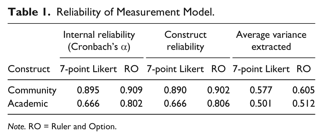
Note. RO = Ruler and Option.

where i represents the item number, n is the total number of items, L_i represents the standardized factor loading for each item, and $\sum_{i = 1}^{n} (1 - L_{i}^{2})$ is the sum of the error variance terms for a construct.

Results in Table 1 show that measurement model using data from RO scale had higher internal reliability, higher internal consistency of the items representing a construct (CR), and higher percentage of variance explained by the items in a construct (AVE) than measurement model using data from 7-point Likert scale.

Validity Coefficients

Three measures of validity, correlation between constructs (measures discriminant validity), model fit indices (measures construct validity), and AVE (measures convergent validity) were used to assess and compare the validity of the measurement models from both data sets (refer to Tables 2 and 3). The values of the three measures of validity show that measurement models from both data are valid. The fit indices for both measurement models achieved the acceptance level (χ² / df < 5 [Marsh & Hocevar, 1985], goodness-of-fit index [GFI] > 0.9 [Joreskog & Sorbom, 1984], adjusted GFI [AGFI] > 0.9 [Tanaka & Huba, 1985], comparative fit index [CFI] > 0.9 [Bentler, 1990], root mean square error approximation [RMSEA] < 0.08 [Arbuckle, 2012]). There were only slight differences in the correlation coefficients between constructs and the model fit indices. Correlation coefficient between constructs for data from 7-point Likert scale was slightly lower (0.71) compared with the correlation coefficient between constructs for data from RO scale (0.72). Similarly, the fit indices of measurement model for data from 7-point Likert scale were slightly better than the fit indices of measurement model for data from RO scale. In Table 3, the diagonal values in bold are the square roots of AVE while other values are the correlation between the constructs. The discriminant validity is achieved when diagonal value in bold is higher than the values in its row and column (Hair et al., 2010). Results showed that measurement model for data using RO scale had higher convergent validity; while both models attain almost the same level of discriminant and construct validity.

Table 2.

Validity of Measurement Model.

	Discriminant validity		Construct validity		Convergent validity
Construct	7-point Likert	RO	7-point Likert	RO	7-point Likert	RO
CommunityAcademic	0.71	0.72	χ² / df = 2.557 GFI = 0.978 AGFI = 0.956 CFI = 0.987 RMSEA = 0.055	χ² / df = 3.098 GFI = 0.965 AGFI = 0.939 CFI = 0.977 RMSEA = 0.064	0.577 0.501	0.605 0.512

Note. RO = Ruler and Option; GFI = goodness-of-fit index; AGFI = adjusted GFI; CFI = comparative fit index; RMSEA = root mean square error approximation.

Table 3.

The Discriminant Index Summary.

Construct	7-point Likert		RO
Construct	Community	Academic	Community	Academic
Community	0.76		0.78
Academic	0.71	0.71	0.72	0.72

Note. RO = Ruler and Option.

Degrees of Freedom and Standardized Residual Covariances

Degrees of freedom (df) is the amount of mathematical information available to estimate the model parameters (Hair et al., 2010). The ratio of df to number of parameters was higher for measurement model using RO scale (32:23) than measurement model using 7-point Likert scale (18:18). In SEM, the df are calculated based on the size of the covariance matrix, not on the sample size. Thus, more df means more mathematical information to estimate model parameters. All the standardized residual covariances for both data sets show good fit with no consistent pattern of large standardized residuals.

Limitations of the Study

The application of stratified random sampling method supports generalization to the population of university students. However, results cannot be generalized to non- university students population.

Conclusions and Recommendations

Being naturally intangible, the task of measuring attitude summons a careful choice of measuring instrument to produce correct and meaningful research results. This article has demonstrated how an interval metric scale can be generated based on three main features (presence of meaningful zero point, presence of measurement unit, and clearly defined operational procedure as the basis for measurement) and named the scale as RO scale. Results from a repeated measurement survey showed that data from RO scale performed better than data from 7-point Likert scale in terms of number of items per construct, factor loadings, squared multiple correlations, higher internal reliability, higher internal consistency of the items representing a construct, and higher percentage of variance explained by the items in a construct. Measurement model using RO scale had higher ratio of df to number of parameters, thus providing more mathematical information to estimate model parameters. In terms of validity coefficients, measurement model using RO scale had higher convergent validity; but measurement models using both scales achieved almost the same level of discriminant and construct validity. Previous study had shown that RO scale was easy to use (on the respondents’ part) and easy to adminster (on the researcher’s part) (Rohana Yusoff & Roziah Mohd Janor, 2012).

Regarding the design of RO scale, the authors would like to remind readers not to be engrossed with the visual form of the ruler because in future, any researcher who is more artistic may come up with a better form that might be more space saving. The only reason why a ruler format was chosen was because it resembles infinite points (portrays continuity) and is easy to relate, as perhaps everyone who has gone to school would be familiar with it. The authors would like to call on readers to focus on the more important agenda in measurement that the scale tries to uphold: precision, objectivity, unambiguousness, and meaningfulness. It is hoped that this article will incite social science researchers to choose a scale along this line of thought. This is because a researcher’s utmost concern is making correct interpretation, meaningful statements, and valid inference on the population. Finally, further studies are needed to elicit the strength and weakness of RO scale to identify the situations where it is most suitable.

Footnotes

Acknowledgements

The authors would like to express gratefulness and thankfulness to the reviewers for their comments that had been of great help in upgrading the writing of the article. Special thanks also goes to Norulhidayah for her strong personal support; to friends, Mazni, Siti Norliana, and Hasiah for their help in translating questionnaire items to Malay language.The authors would also like to thank everyone who has participated in this research and to the university for providing the fund and facilities.

Authors’ Note

This article is a revised and extended version of the article titled “A Proposed Metric Scale for Expressing Opinion,” which was presented at the International Conference on Statistical in Science, Business and Engineering (2012).

Declaration of Conflicting Interests

The author(s) declared no potential conflicts of interest with respect to the research, authorship, and/or publication of this article.

Funding

The author(s) disclosed receipt of the following financial support for the research, authorship, and/or publication of this article: This study received financial support from ‘Dana Kecemerlangan UiTM’ (UiTM Excellence Fund) 600-UiTMKD (PJI/RMU/ST/DANA 5/2/1/DST (9/2012).

Author Biographies

Rohana Yusoff is a senior lecturer in Statistics at Faculty of Computer Sciences & Mathematics, Universiti Teknologi MARA Terengganu.

Roziah Mohd Janor is an Associate Professor in Statistics at Faculty of Computer Sciences & Mathematics, Universiti Teknologi MARA Shah Alam. She is currently the Director of Curriculum Affairs Academic Affairs Division, Universiti Teknologi MARA and Associate Fellow at ipromise and MITRAN.

References

Agresti

(2002). Categorical data analysis (2nd ed.). Hoboken, New Jersey: John Wiley & Sons.

Aguinis

Pierce

C. A.

Culpepper

S. A.

(2009). Scale coarseness as a methodological artifact. Organizational Research Methods, 12, 623-652.

Aitken

R. C. B.

(1969). Measurement of feelings using visual analogue scales. Proceedings of the Royal Society of Medicine, 62, 989-993.

Albaum

(1997). The Likert scale revisited: An alternate version. Journal of the Market Research Society, 39(2), 331-348.

Amah

(2013). Employee involvement and organizational effectiveness. Journal of Management Development, 32, 661-674. doi:10.1108/jmd-09-2010-0064

Arbuckle

J. L.

(2012). IBM® SPSS® Amos™ 21 User’s Guide. Amos Development Corporation. Retrieved from http://www.google.com.my/url?sa=t&rct=j&q=&esrc=s&frm=1&source=web&cd=1&ved=0CCsQFjAA&url=ftp%3A%2F%2Fpublic.dhe.ibm.com%2Fsoftware%2Fanalytics%2Fspss%2Fdocumentation%2Famos%2F21.0%2Fen%2FManuals%2FIBM_SPSS_Amos_Users_Guide.pdf&ei=PT2jUtj9LoqtiAfEk4HADQ&usg=AFQjCNHzVc8UR4b_Yfag5XbKc5NPb2m6MQ&bvm=bv.57752919,d.dGI

Ayesh

(2004, October 10-13). Emotionally motivated reinforcement learning based controller. Paper presented at the IEEE International Conference on Systems, Man and Cybernetics, The Hague, The Netherlands.

Babbie

(2001). The practice of social research (9th ed.). Belmont, CA: Wadsworth Thomson.

Barrett

P. T.

(2003). Beyond psychometrics: Measurement, non-quantitative structure, and applied numerics. Journal of Managerial Psychology, 3, 421-439.

10.

Bentler

P. M.

(1990). Comparative fit indexes in structural models. Psychological Bulletin, 107, 238-246.

11.

Bevan

(2003). What is usability? Retrieved from http://www.usabilitynet.org/management/b_what.htm

12.

Bharadwaj

(2007). Development of a Fuzzy Likert Scale for the WHO ICF to include categorical definitions on the basis of a continuum. Wayne State University. Retrieved from http://digitalcommons.wayne.edu/dissertations/AAI1442894, (AAI1442894)

13.

Boone

H. N.

Jr. Boone

D. A.

(2012). Analyzing Likert data. Journal of Extension, 50(2), Article 2TOT2.

14.

Cella

D. F.

Perry

S. W.

(1986). Reliability and concurrent validity of three visual-analogue mood scales. Psychological Reports, 59, 827-833.

15.

Chang

(2009). Operationalism. In Zalta

E. N.

(Ed.), The Stanford Encyclopediaof Philosophy (January-March, 2009 ed.). Retrieved from http://plato.stanford.edu/archives/fall2009/entries/operationalism/

16.

Chimi

C. J.

Russell

D. L.

(2009, November). The Likert scale: A proposal for improvement using quasi-continuous variables. Paper presented at the ISECON 2009, Washington, DC.

17.

Cicchetti

D. V.

Shoinralter

Tyrer

P. J.

(1985). The effect of number of rating scale categories on levels of interrater reliability: A Monte Carlo investigation. Applied Psychological Measurement, 9, 31-36. doi:10.1177/014662168500900103

18.

Clogg

C. C.

Shihadeh

E. S.

(1994). Statistical models for ordinal variables (Advanced Quantitative Techniques in the Social Sciences) (1st ed.). Thousand Oaks, CA: Sage.

19.

Cox

E. P.

(1980). The optimal number of response alternatives for a scale: A review. Journal of Marketing Research, XVII, 407-422.

20.

Davison

M. L.

Sharma

A. R.

(1988). Parametric statistics and levels of measurement. Psychological Bulletin, 104, 137-144.

21.

Diller

A. N. N.

(1975). On tacit knowing and apprenticeship. Educational Philosophy and Theory, 7(1), 55-63. doi:10.1111/j.1469-5812.1975.tb00507.x

22.

Dolnicar

Grun

(2007). How constrained a response: A comparison of binary, ordinal and metric answer formats. Journal of Retailing and Consumer Services, 14, 108-122.

23.

Fabrigar

L. R.

Paik

J. S.

(2013). Thurstone scales. In Salkind

N. J.

(Ed.), Encyclopedia of measurement and statistics (pp. 1003-1006). Thousand Oaks, CA: Sage. doi:10.4135/9781412952644.n457

24.

Fadiya

O. O.

(2013). Analysing the perceptions of UK building contractors on the contributors to the cost of construction plant theft. Journal of Financial Management of Property and Construction, 18, 128-141. doi:10.1108/jfmpc-10-2012-0039

25.

Fauziah

M. J.

Rosna

A. H.

Tengku Faekah

T. A.

(2012). Malaysian University Student Learning Involvement Scale (MUSLIS): Validation of a student engagement model. Malaysian Journal of Learning & Instruction, 9, 15-30.

26.

Ferrando

P. J.

(2003). A Kernel density analysis of continuous typical-response scales. Educational and Psychological Measurement, 63, 809-824.

27.

Gao

Mokhtarian

P. L.

Johnston

R. A.

(2008). Nonnormality of data in structural equation models. Transportation Research Record: Journal of the Transportation Research Board, 2082(1), 116-124.

28.

Garland

(1990). A comparison of three forms of the semantic differential. Marketing Bulletin, 1, 19-24, Article 14.

29.

Geramian

S. M.

Mashayekhi

Ninggal

M. T. B. H.

(2012). The relationship between personality traits of international students and academic achievement. Procedia—Social and Behavioral Sciences, 46, 4374-4379.

30.

Gordon

J. S.

Mahabee-Gittens

E. M.

Andrews

J. A.

Christiansen

S. M.

Byron

D. J.

(2013). A randomized clinical trial of a web-based tobacco cessation education program. Pediatrics, 131, 455-462.

31.

Grace

(2008). Can Likert scale data ever be continuous? Retrieved from http://www.articlealley.com/article_670606_22.html

32.

Granberg-Rademacker

J. S.

(2010). An algorithm for converting ordinal scale measurement data to interval/ratio scale. Educational and Psychological Measurement, 70, 74-90.

33.

Guyat

G. H.

Townsend

Berman

L. B.

Keller

J. L.

(1987). A comparison of Likert and visual analogue scales for measuring change in function. Journal of Chronic Diseases, 40, 1129-1133.

34.

Hair

Joseph F.

Jr. Black

William C.

Babin

Barry J.

Anderson

Rolph E.

(2010). Multivariate data analysis (7th ed.). Upper Saddle River, New Jersey: Pearson Prentice Hall.

35.

Hand

D. J.

(1996). Statistics and the theory of measurement. Journal of the Royal Statistical Society, 159, 445-492.

36.

Harwell

M. R.

Gatti

G. G.

(2001). Rescaling ordinal data to interval data in educational research. Review of Educational Research, 71, 105-131.

37.

Hawkins

D. I.

Albaum

Best

(1974). Stapel scale or semantic differential in marketing research? Journal of marketing research, 11(3), 318-322.

38.

Heise

D. R.

(1969). Some methodological issues semantic differential research. Psychological Bulletin, 72, 406-422. doi:10.1037/h0028448

39.

Henson

R. K.

Hull

D. M.

Williams

C. S.

(2010). Methodology in our education research culture. Educational Researcher, 39, 229-240. doi:10.3102/0013189x10365102

40.

Hsu

Chang

Hung

H. F.

(2007, December 2-5). Applying SVM to build supplier evaluation model-comparing Likert scale and Fuzzy scale. Paper presented at the IEEE IEEM, Singapore.

41.

Jain

(2013). An instrument to measure factors of strategic manufacturing effectiveness based on Hayes and Wheelwright’s model. Journal of Manufacturing Technology Management, 24, 812-829. doi:10.1108/jmtm-11-2011-0102

42.

Jamieson

(2004). Likert scales: How to (ab)use them. Medical Education, 38, 1212-1218.

43.

Joreskog

K. G.

Sorbom

(1984). LISREL VI user’s guide. Mooresville, IN: Scientific Software.

44.

Kemp

Grace

R. C.

(2010). When can information from ordinal scale variables be integrated? Psychological methods, 15, 398-412.

45.

Kline

R. B.

. (1998). Principles and practice of structural equation modeling. New York: Guilford.

46.

Kline

R. B.

(2005). Principles and practice of structural equation modeling (2nd ed.). New York, NY: Guilford.

47.

Knapp

T. R.

(1990). Treating ordinal scales as interval scales: An attempt to resolve the controversy. Nursing Research, 39(2), 121-123.

48.

Kornfeld

(2013). Selection of lean and six sigma projects in industry. International Journal of Lean Six Sigma, 4, 4-16. doi:10.1108/20401461311310472

49.

Lerdal

Kottorp

Gay

C. L

Lee

K. A.

(2013). Lee fatigue and energy scales: Exploring aspects of validity in a sample of women with HIV using an application of a Rasch model. Psychiatry research, 205, 241-246.

50.

Lietz

(2010). Research into questionnaire design. International Journal of Market Research, 52(2), 249-272.

51.

Mann

P. S.

(2001). Introductory statistics (4th ed.). New York, NY: Wiley.

52.

Marcus-Roberts

H. M.

Roberts

F. S.

(1987). Meaningless statistics. Journal of Educational and Behavioral Statistics, 12, 383-394.

53.

Markus

K. A.

Borsboom

(2011). The cat came back: Evaluating arguments against psychological measurement. Theory & Psychology. 22, 452-466. doi:10.1177/0959354310381155

54.

Marsh

H. W.

Hocevar

(1985). Application of confirmatory factor analysis to the study of self-concept: First-and higher-order factor models and their invariance across groups. Psychological Bulletin, 97, 562-582.

55.

Matheson

(2008, December). I can’t believe it’s not measurement: The legacy of operationism in social-scientific uses of numbers. Paper presented at the TASA 2008 Conference, University of Melbourne, Australia.

56.

Meulman

J. J.

(1998). Optimal scaling methods for multivariate categorical data analysis. Available from http://www.spss.com

57.

Michell

(1986). A clash of paradigms. Psychological bulletin, 100, 398-407.

58.

Michell

(1997). Quantitative science and the definition of measurement in psychology. British Journal of Psychology, 88, 355-383. doi:10.1111/j.2044-8295.1997.tb02641.x

59.

Michell

(1999). Measurement in psychology: A critical history of a methodological concept. New York, NY: Cambridge University Press.

60.

Munshi

(1990). A method for constructing Likert scales. Retrieved from http://www.munshi.4t.com/papers/likert.html

61.

Norman

(2010). Likert scales, levels of measurement and the “laws” of statistics. Advances in health sciences education, 15, 625-632.

62.

Pennebaker

J. W.

Czajka

J. A.

Cropanzano

Richards

B. C.

Brumbelow

Ferrara

. . . Thyssen

(1990). Levels of thinking. Personality and Social Psychology Bulletin, 16, 743-757.

63.

Pfennings

Cohen

van der Ploeg

(1995). Preconditions for sensitivity in measuring change: Visual analogue scales compared to rating scales in a Likert format. Psychological Reports, 77, 475-480.

64.

Presser

Schuman

(1989). The management of a middle position in attitude surveys. In Presser

E. S. A. S.

(Ed.), Survey research methods (pp. 108-123). Chicago, IL: University of Chicago.

65.

Preston

C. C.

Colman

A. M.

(2000). Optimal number of response categories in rating scales: Reliability, validity, discriminating power, and respondent preferences. Acta Psychologica, 104, 1-15.

66.

Puzziawati

Ghani

Abdul Aziz

(2005). Quantifying priority in women’s decision-making. Jurnal Teknologi, 42(E), 19-30.

67.

Razzaque

M. A.

(2013). Religiosity and Muslim consumers’ decision-making process in a non-Muslim society. Journal of Islamic Marketing, 4, 198-217. doi:10.1108/17590831311329313

68.

Yusoff

Rohana

Janor

Roziah Mohd

. (2012). A proposed metric scale for expressing opinion. Paper presented at the International Conference on Statistics in Science, Business and Engineering (ICSSBE 2012), Langkawi, Kedah, Malaysia.

69.

Russell

Gary J.

(2010). Itemized Rating Scales (Likert, Semantic Differential, and Stapel). Wiley International Encyclopedia of Marketing (pp. 138-146): John Wiley & Sons, Ltd. Retrieved from http://dx.doi.org/10.1002/9781444316568.wiem02011. doi: 10.1002/9781444316568.wiem02011

70.

Sarafidou

J. O.

(2013). Teacher participation in decision making and its impact on school and teachers. International Journal of Educational Management, 27, 170-183. doi:10.1108/09513541311297586

71.

Sarle

W. S.

(1997). Measurement theory: Frequently asked questions. Retrieved from ftp://ftp.sas.com/pub/neural/measurement.html

72.

Scherpenzeel

A. C.

Saris

W. E.

(1997). The validity and reliability of survey questions. Sociological Methods & Research, 25, 341-383. doi:10.1177/0049124197025003004

73.

Stevens

S. S.

(1946). On the theory of scales of measurement. Science In Stevens

S. S.

(Ed.), Handbook of Experimental Psychology (Vol. 103, pp. 677-680). New York: Wiley.

74.

Stevens

S. S.

(1951). Mathematics, measurement, and psychophysics. In Stevens

S. S.

(Ed.), Handbook of experimental psychology (pp. 1-49). New York: Wiley.

75.

Stevens

S. S.

(1959). Measurement, Psychophysics and Utility. In Churchman

C. W.

Ratoosh

(Eds.), Measurement: Definitions and Theories. New York: John Wiley.

76.

Skow

(2011). Does temperature have a metric structure? Philosophy of Science, 78, 472-489.

77.

Stone

Stenner

(2012). On temperature. Rasch Measurement Transactions, 26, 1351-1353.

78.

Suppes

Zinnes

J. L.

(1963). Basic measurement theory. Handbook of mathematical psychology, 1, 1-76.

79.

Tanaka

J. S.

Huba

G. J.

(1985). A fit index for covariance structure models under arbitrary GLS estimation. British Journal of Mathematical and Statistical Psychology, 38, 197-201.

80.

Trendler

(2009). Measurement theory, psychology and the revolution that cannot happen. Theory & Psychology, 19, 579-599. doi:10.1177/0959354309341926

81.

Vagias

W. M.

(2006). Likert-type scale response anchors. Department of Parks, Recreation and Tourism Management, Clemson International Institute for Tourism & Research Development, Clemson University. Retrieved from http://www.clemson.edu/centersinstitutes/tourism/documents/sample-scales.pdf

82.

Velleman

P. F.

Wilkinson

(1993). Nominal, ordinal, interval, and ratio typologies are misleading. The American Statistician, 47, 65-72.

83.

Weston

Gore

P. A.

Jr. (2006). A brief guide to structural equation modeling. The counseling psychologist, 34, 719-751. doi:10.1177/0011000006286345

84.

Wildt

A. R.

Mazis

M. B.

(1978). Determinants of scale response: Label versus position. Journal of Marketing Research, 15(2), 261-267.

85.

Wilson

L. N.

Wainwright

G. A.

Stehly

C. D.

Stoltzfus

Hoff

W. S.

(2013). Assessing the academic and professional needs of trauma nurse practitioners and physician assistants. Journal of Trauma Nursing. 20, 51-55. doi:10.1097/JTN.0b013e31828661e9

86.

C. H.

(2007). An empirical study on the transformation of Likert scale data to numerical scores. Applied Mathematical Sciences, 1, 2851-2862.

87.

Zaimah

Sarmila

M. S.

Lyndon

Azima

A. M.

Selvadurai

Saad

A. C.

(2013). Financial behaviors of female teachers in Malaysia. Asian Social Science, 9(8), 34-41. doi:10.5539/ass.v9n8p34

Generation of an Interval Metric Scale to Measure Attitude

Abstract

Keywords

Review of Literatures

Measurement Theories

Discrete, Continuous, and Ordinal Variables

Measurement Scales in Social Science

Shortcomings of Likert Scale

Approaches Offered by Researchers

Mathematical modeling

Continuous line segments

Scales for Measuring Attitude Should Be Continuous

Usability of Rating Scales

Generation of a Metric Interval Scale

Method

Results and Discussion

Mean Values, Standard Deviations, and Skewness of Items

Number of Indicator Items Per Construct, Factor Loadings, Squared Multiple Correlations (R2), and Reliability Coefficients of Items

Validity Coefficients

Degrees of Freedom and Standardized Residual Covariances

Limitations of the Study

Conclusions and Recommendations

Footnotes

Acknowledgements

Authors’ Note

Declaration of Conflicting Interests

Funding

Author Biographies

References

Number of Indicator Items Per Construct, Factor Loadings, Squared Multiple Correlations (R²), and Reliability Coefficients of Items