Sage Journals: Discover world-class research

Abstract

Developing models to predict the effects of social and economic change on agricultural landscapes is an important challenge. Model development often involves making decisions about which aspects of the system require detailed description and which are reasonably insensitive to the assumptions. However, important components of the system are often left out because parameter estimates are unavailable. In particular, measurements of the relative influence of different objectives, such as risk, environmental management, on farmer decision making, have proven difficult to quantify. We describe a model that can make predictions of land use on the basis of profit alone or with the inclusion of explicit additional objectives. Importantly, our model is specifically designed to use parameter estimates for additional objectives obtained via farmer interviews. By statistically comparing the outputs of this model with a large farm-level land-use data set, we show that cropping patterns in the United Kingdom contain a significant contribution from farmer’s preference for objectives other than profit. In particular, we found that risk aversion had an effect on the accuracy of model predictions, whereas preference for a particular number of crops grown was less important. While nonprofit objectives have frequently been identified as factors in farmers’ decision making, our results take this analysis further by demonstrating the relationship between these preferences and actual cropping patterns.

Keywords

agriculture multiattribute utility theory socioeconomic model stated preferences

Introduction

Models of agricultural land use are often used to predict how future landscapes will reflect farmers’ responses to social, economic, technological, or environmental change, and so inform policy decisions. Examples include efforts to understand the implications of potential incentives for greenhouse gas mitigation on agriculture (Perez & Muller-Holm, 2001) and in predicting the effects of agricultural policy on biodiversity (Pacini, Wossink, Geisen, & Huirne, 2004; Watkinson, Freckleton, Robinson, & Sutherland, 2000).

Central to most land-use models are assumptions about the behavior of farmers and, in particular, about the decision-making process adopted when choosing crops. In the vast majority of models (including the one described here), farmers are assumed to act so as to optimize a utility function. When constructing this utility function, modelers must make decisions about which aspects of farmer behavior to include, and which to exclude, as well as how parameters will be estimated and how the utility function itself will be solved. Models that attempt to predict the effects of policy changes are often constructed using the technique of mathematical programming because this accommodates legislated requirements and subsidies relatively easily.

Two major variants of agricultural mathematical programming models have emerged. The oldest involves explicitly specifying as many aspects of the farming profit function as possible, such as rotational constraints, timing of field operations, diseases, and environmental runoff (see, for example, Annetts & Audsley, 2002; Arfini, 2005; Rounsevell, Annetts, Audsley, Mayr, & Reginster, 2003). One advantage of this explicit modeling approach is that, because underlying processes are modeled explicitly, these models should be more robust to predicting land use in novel policy scenarios. The disadvantage of this approach is that it is often extremely difficult to quantify all of the required parameters in such an explicit model, and there are inevitably aspects of the system that are omitted. As a consequence, early explicit models were found to have limited predictive accuracy, which led to the development of “Positive Mathematical Programming” (PMP; Howitt, 1995), in which a relatively simple utility function is constructed, and a quadratic correction function is found that exactly calibrates the model to reference data. In a PMP model, aspects of the system that are difficult to quantify get subsumed into the correction term. Although this means that even relatively simple PMP models can appear to have good predictive qualities, it also means that the ability of the model to make predictions outside the circumstances of the reference data set is limited. PMP and explicit models therefore serve complementary functions in predictive modeling, and it is important that both are pursued. In this article, we focus on explicit models because our goal is to evaluate the importance of particular aspects of farmer’s behavior in determining land use.

As farming is a business activity, it is not surprising that many explicit models of farmer behavior have focused purely on the contribution of profit to utility (Janssen & van Ittersum, 2007). There is, however, considerable qualitative evidence that farmers also make land-use decisions in response to a variety of nonprofit objectives such as maintaining independence (Gasson, 1973), controlling workload (Fairweather & Keating, 1994; Solano, Léon, Pérez, & Herrero, 2001), reducing risk (Harper & Eastman, 1980; McGregor et al., 1996; Solano et al., 2001), and caring for the environment (Brodt, Klonsky, & Tourte, 2006; Fairweather & Keating, 1994; Solano et al., 2001). While these studies collectively suggest that farmers value outcomes other than pure profit, there is currently very little quantitative evidence to assess whether this translates to observed behavior. To address this problem, detailed quantitative studies are required across different farming contexts examining the question of whether farmer’s stated preferences correlate with observed behavior.

Our goal here is to examine the importance of preferences other than profit in determining crop composition for lowland arable farmland in England and Wales. Specifically, we aim to determine whether the addition of key nonprofit preferences to the utility function of farmers can improve the agreement between model outputs and empirical data. To achieve this, we develop a method for including multiple preferences in the utility function of farmers that is closely tied to an interview process eliciting parameters for the model. We then make use of a detailed and extensive data set, the Farm Business Survey (Department for Environment, Food and Rural Affairs & National Assembly for Wales, 2002, 2003, 2004, 2005; Ministry of Agriculture, Fisheries and Food & National Assembly for Wales, 2001), which provides information on crop yields and areas grown at the individual farm holding level. Model performance can be assessed based on agreement between model predictions and the survey data. We compare the performance of a range of models, including a purely empirical benchmark (a regression of crop gross margin against area), a pure-profit model, and a model incorporating multiple preferences.

We begin by describing the model itself in three parts: (a) the framework for constructing a single weighted objective (utility) from a number of subobjectives, (b) how key preferences were identified and quantified, and (c) how these are implemented within our model. We then describe the methods used to compare model output with empirical data.

Trading-Off Multiple Objectives: Mathematical Framework

The core of the model is a description of individual farmer decision making that assumes the selected decision optimizes a weighted combination of all relevant objectives. We used mixed-integer programming for this because it is suited to the inclusion of multiple objectives and is widely used in land-use simulation models (Arfini, 2005). A linear or mixed-integer programming model comprises an overall objective function to be maximized or minimized subject to a series of constraints (Press, Teukolsky, Vetterling, & Flannery, 1992). The overall objective function is a simple sum of the following form:

U = \sum_{i} c_{i} x_{i} .

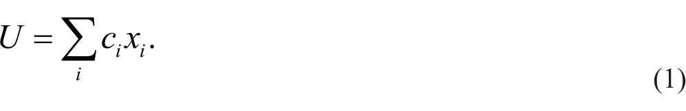
In our model, U is overall utility and x_i denotes the quantity of various units, such as areas of crops, number of workers, or number of machines. The constants, c_i , are the amount of utility gained or lost for a change in x_i and include crop gross margins, labor costs, and machinery costs. For any given farm, there are constraints on the potential values of x_i , such as the amount of labor or equipment time available. Nonlinear relationships can be incorporated through a system of constraints and integer variables called “special ordered sets” (Beale & Forrest, 1976). As special ordered sets can substantially increase computation time, we minimized their use by describing curved objective functions (see below) with a small (<4) number of line segments.

The utility model comprises multiple objectives, such as profit, risk, and crop complexity, each of which is a sum of contributions from each of the quantities x_i . This leads to a hierarchy of sums:

U = u_{k} w_{k} \sum_{k} O_{k},

O_{k} = \sum_{i} c_{i}^{k} x_{i},

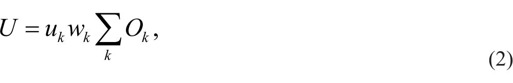
where each of the k objectives, O_k , is associated with two constant factors, u_k and w_k . The factor, u_k , converts the units of objective k (e.g., profit, risk, or crop complexity) into a common scale based on utility (see below for a description of how each individual objective is calculated). The weighting w_k determines the importance of objective k relative to the other objectives. Values are renormalized so that $Σ_{k} w_{k} = 1$ . Each of the individual k objectives has an associated set of coefficients, $c_{i}^{k}$ determining the contribution from each x_i to that objective. The solution consists of a vector $X = {x_{1}, x_{2}, \dots x_{n}}$ describing the optimal land-use configuration. For nonlinear relationships between U and O_k , a special ordered set constraint is applied, which ensures that an appropriate value of u_k is used according to the value of O_k in different segments of the curve.

The model is implemented as a package, “farmR” for the open source statistical environment, R (R Development Core Team, 2008). It uses the open source COIN-LP (http://www.coin-or.org/) numerical library to solve the underlying mixed-integer programming problem. The package, including source code, is available from the Comprehensive R Archive Network (http://cran.r-project.org/src/contrib/Archive/farmR).

Estimation of Preferences

Although the parameters w_k and u_k for each objective are indistinguishable in mathematical terms (see Equation 2), we distinguish between them in our framework because they are conceptually different and must therefore be elicited separately.

Prior to the interviews, we identified 15 farm management objectives based on a literature review, pilot farmer interviews, and a focus group (a complete list of objectives is provided in Appendix A). Subsequently, detailed interviews were conducted using a multicriteria decision analysis framework (Belton & Stewart, 2002) with 47 farmers from the eastern counties of England (Bedfordshire, Lincolnshire, and Norfolk) to elicit model parameters. The interactive software, Logical Decisions® Version 5.129 (http://www.logicaldecisions.com), was used to record data and allow farmers to view their results and revise them if required. Logical Decisions is a decision support software based on multicriteria decision making used to implement the Analytic Hierarchy Process (see, for example, Moffett, Dyer, & Sarkar, 2006). It was used with our farmers to interactively work through the objective hierarchy and record data, and allowed the farmers to instantaneously view results, provide feedback, and modify their responses iteratively until satisfied. For each objective, the farmers were asked to state the two objective values at which they would experience 0% and 100% satisfaction (utility). The farmers were then asked to identify their satisfaction level at between 1 and 6 intermediate points, resulting in a satisfaction curve. This process provided values for u_k : the slope of the relationship between utility and the kth objective at the various positions along the curve.

Following capture of satisfaction curves, a SMART/SWING weighting procedure was carried out (Mustajoki, Hämäläinen, & Salo, 2005; von Winterfeldt & Edwards, 1986). The farmers were asked to state the objective that they most wished to move from its worst (0% satisfaction) to its best (100% satisfaction) level. This objective, which was almost always profit, was given a score of 100 and the importance of moving every other objective, from the worst to the best level, was scored relative to it. After completing this process once, the results were normalized so that the sum of all preference weights was equal to 1. Upon viewing the normalized results, the farmers were given the opportunity to revise their estimates until satisfied that the weights reflected their preferences. This section of the interview provided a set of weights w_k for each objective.

Choice of Objectives and Calculation of Weights

Of the 15 objectives assessed, the most important were profit (defined as the sum of revenues and subsidies, less variable costs), risk minimization, free time (defined as time not farming), and crop management complexity (defined as the total number of crop types grown). Together, these accounted for more than 50% of preference weights. Although free time was listed as second most important on average, simple models of free time (based on number of free days per year) were saturated (achieved 100% satisfaction with respect to the objective) without any adjustments to crop choice; the objective was therefore excluded from further consideration. Our model almost certainly does not represent free time well because it does not include time spent on administration, account for time saved through the use of contractors, or include preferences for the timing with which free time is taken. We were unable to include such a detailed free time model in the present study because we did not have access to detailed data on administration time or farmers’ preferences for timing of free time. By leaving this component out of our objective function, we make the assumption that it is relatively orthogonal to the other major objectives under consideration. The model therefore included the three important objectives: profit, risk minimization, and crop management complexity. The remaining objectives were given low weightings; including them would have added considerable complexity to the model.

The average relative preference weights were profit, 24%; perceived risk, 9%; and crop management complexity, 8.5%. When rescaled such that profit was equal to 100%, the weights were 37% for risk and 35% for crop complexity. Throughout the remainder of the article, we refer to objective weightings assuming that this rescaling has been applied.

Satisfaction Curves

The satisfaction curve for each objective is the relationship between utility (U) and the objective value. Each of the farmers in our stated preference survey gave an individual satisfaction curve for each objective, and we used averages of these curves when calculating model outputs for the Farm Business Survey farmers. This average curve was determined by fitting a spline function to the curve of each farmer, choosing a standard set of x values, and then averaging the y values at each x. To incorporate these curves into our model, we converted each curve into between 1 and 4 linear segments (depending on the objective), giving a set of slopes (u_k ).

The average stated profit curve (standardized to a 250-ha farm) was a straight line between £0 (0% satisfaction) and £120,000 (100% satisfaction). These values were elicited from farmers using the methods described above and represent the average points at which a farmer’s satisfaction would be saturated (maximum) and fall to 0 (minimum). However, for inclusion in the model, the values of the parameter determined from the intercept had to be adjusted to take account of the fact that the model objective function predicts net gross margin (defined as the sum of crop gross margins minus labor and machinery costs) and not profit. This difference is because various fixed costs, such as rent, insurance, building repairs, and administrative costs, are excluded. The model gave a minimum net gross margin of £60,000 (across the Farm Business Survey input values); among farmers, in our stated preference survey, the minimum expected profit was £0. We therefore applied an offset to the profit-utility curve of £60,000 corresponding to the difference between a farmer’s stated minimum profit and the minimum profit objective (net gross margin) that was output by the model. This resulted in a recalibrated profit-utility curve so that 0% satisfaction was achieved at a profit of £60,000 and 100% satisfaction was achieved at £180,000.

Stated satisfaction curves for risk among farmers were almost always linear, with decreasing relationships differing in intercepts. To summarize this pattern, we first chose the x intercept by finding the average risk value at which the farmer’s satisfaction was 0% (£116,000). We then found the risk value at which satisfaction first dropped below 100% (£37,000). Our final curve was then a line with two segments—one from risk = 0, satisfaction = 100% to risk = £37,000, satisfaction = 100% and one from risk = £37,000, satisfaction = 100% to risk = £116,000, satisfaction = 100%.

During pilot interviews, farmers identified the number of different crops grown as an important and measurable indicator of management complexity. Hence, we used the number of different crop types grown as a measure of crop management complexity. The relationship between this quantity and overall utility was more complex than for profit or risk minimization because different farmers had three qualitatively different curve shapes. One group preferred to minimize the number of crops grown (monotonic decreasing curve), another group preferred an intermediate number (humped curve), and the remaining farmers preferred to maximize the number of crops grown within the range available (monotonic increasing curve). The proportion of farmers in each group was 31%, 50%, and 19%, respectively. To translate this into a form suitable for the model, we calculated an average curve (utility against crop number) for each group. The actual curves used are shown in Figure 1, and all cropping predictions made from our model were calculated as weighted sums of solutions for each of the three farmer preference types.

Figure 1.

Average stated preference curves for crop management complexity showing three different groups of farmers.

Model Components for Specific Objectives

Profit Objective

We use a profit model (see Annetts & Audsley, 2002; Rounsevell et al., 2003, for a full description) to calculate income generation from an arable farm. The profit objective (defined as annual net gross margin) of this model is the sum,

O_{profit} = \sum_{i} G_{i} a_{i} + \sum_{i j k} C_{i j k} x_{i j k} + \sum_{m} C_{m} n_{m},

which is composed of three parts: the gross margin, G_i , for each crop; the costs, C_ijk , of each field operation, including any timeliness penalty (the jth operation on crop i in period k); and the costs, C_m , of the machines and labor required to perform the field operations. The model variables are a_i , the area of crop i; x_ijk , the area of operation, j, on crop i in period k; and the number of machines n_m of type m. Each variable is accompanied by its corresponding coefficient.

A series of constraints is applied to ensure that only realistic solution vectors are obtained when maximizing the profit objective (Equation 4). These constraints have previously been described in detail by Rounsevell et al. (2003) and Annetts and Audsley (2002). In summary, they ensure that the following conditions are met: (a) total land area is constant, (b) all necessary field operations are performed for each crop in the required sequence, (c) the labor and machinery required to perform field operations do not exceed that available, and (d) that crops are rotated such as to prevent the buildup of diseases and pests. These constraints and their associated parameters form the model’s description of the farming system. Parameters include commodity prices, machinery work rates, rotational constraints on crops, and the timing of agricultural operations required to bring a crop to harvest. The parameters come from a wide variety of sources, the details of which are provided in Appendix B (Table B1). The exact parameter values used are available as online supplementary material.

The model is based on a description of farming at the level of a single operation and assumes that the soil type and rainfall are constant across the entire farm. As large farms may include land with a variety of soil types, we used a weighted average solution over the soil types present in the county where the farm was located. Yearly rainfall was taken to be the average for that county. Soil type and rainfall affect the work rates for various operations, and the amount of time available for fieldwork in each fortnight of the year. In cases where crop yield values were not available from the Farm Business Survey for a particular farmer, a calculation based on soil type and rainfall was used to obtain a predicted yield. This calculation was performed by extrapolating between worst and best expected yields for a crop (Agro Business Consultants, 2004; Nix, 2007) assuming that light soils have the lowest yields and heavy soils the highest. Soil types were calculated based on the methodology described in Rounsevell et al. (2003).

Risk Minimization Objective

We included a risk objective in our model following the basic principle of minimization of total absolute deviation in profits (Hazell, 1971). This is an approximation to the true risk in whole-farm profit because it does not explicitly account for the “risk spreading” that occurs when farmers grow a range of crops with uncorrelated deviations. In our model, the risk objective was calculated according to the formula:

O_{risk} = λ \sum_{i} x_{i} σ_{i},

where the sum is over all crops, x_i is the area of the ith crop, σ_i is the standard deviation in output (price times yield) per hectare for the ith crop, and λ is a constant factor (explained below). In interviews, farmers were asked to specify their stated preference for risk. It is unrealistic to expect interview participants to conceptualize risk directly in mathematical terms, so they were instead asked to envisage a series of scenarios in which the range of their farm income (difference between minimum and maximum over a period of 3-4 years) varied from £0 (minimum) up to the maximum range they would expect. While this definition is different from that used in our model, we assume that the two are related by the constant factor, λ. To estimate λ, we make the following approximate argument.

First, the expected deviation in whole-farm profit will be less than the sum of absolute deviations in profitability of the different crops grown. As farmers grow five crops on average (as indicated by the Farm Business Survey) and assuming that crop outputs vary independently, the whole-farm risk should equal the deviation in the average income from five independently varying values. Thus, the sample standard deviation of effective total profit should roughly equal $σ/ \sqrt{5}$ , where σ is the area-weighted average of standard deviations of individual crops. We assumed that farmers considered the maximum and minimum possible values of their income based on 10 years experience (many farmers had much more experience farming, but as farm technology and policies change rapidly, we assumed that this was a reasonable relevant range). We related this to the standard deviation in crop profitability by considering a sample of 10 independent years from a distribution with standard deviation σ_i and calculating the range of the sample numerically. The result of this calculation was 3.1σ_I. Combining this with the fact that risks are spread among crops, we obtain an approximate value of λ equal to 1.4. This value is clearly approximate, so we examined values of λ from 0.5 to 2.0 in increments of 0.5. The value that resulted in the best fit to data (after also minimizing the sum of squared differences over risk and crop complexity preferences) was λ = 1.0; we used this value in all subsequent analyses.

Statistical Methodology for Comparing Land-Use Data With Model Outputs

Empirical Data Used

We compared the outputs of the socioeconomic model with a large national data set, the Farm Business Survey (Department for Environment, Food and Rural Affairs & National Assembly for Wales, 2002, 2003, 2004, 2005; Ministry of Agriculture, Fisheries and Food & National Assembly for Wales, 2001). The Farm Business Survey is an annual survey of farm businesses across the United Kingdom, including around 3,000 farms in England and Wales. We used the data from England and Wales in this study. Information is provided on an individual farm basis and includes the area, yield, and sale price of each crop grown but not the precise location of the farm. For this analysis, we selected lowland arable farms. Specifically, we included farmers whose holdings were largely below 300 m altitude and for whom arable crops and set-aside accounted for more than 85% of their farmed area. From this sample, we excluded farms <100 ha, because off-farm income probably constitutes a significant portion of the farm business in such cases.

As the farming model makes predictions about long-term cropping, we used average crop areas in the time period 2000 to 2004, calculated individually for each farm. We chose this period to avoid modeling farmer responses to the introduction of the single farm payment (introduced in 2005), because the long-term effects of this policy are unlikely to be apparent during its introductory phase, and it would therefore provide inappropriate data for comparison with our equilibrium model. Farms were excluded if more than 2 years’ data were missing in the 2000 to 2004 time period. The final data set included individual average crop areas between 2000 and 2004 for 149 farms.

We configured the model to predict land use for eight crops (including bare fallow/set-aside) with a combined area that accounts for approximately 85% of arable land in England (Department for Environment, Food and Rural Affairs, 2008). Crops were winter wheat, winter oilseed rape, winter barley, spring barley, legumes (arable pea and bean crops), sugar beet, and potatoes. We also included temporarily unused “set-aside” land. All our comparisons between simulated and actual land use were made relative to the area of these land-use types.

Model Runs

To generate cropping predictions for each farm, we used the time-averaged crop yield values for each farm in our sample from the Farm Business Survey, as inputs for our socioeconomic model. Other than soil type and rainfall (which varied by county), all other variables were kept fixed across farms. In cases where a farmer did not grow a particular crop, we allowed the model to generate yield values for that crop based on soil type and rainfall (see “Profit Objective” section). As the location of farms in the Farm Business Survey was only known to county level, we used a weighted average of model results for each of the soil types and rainfalls present in that county. An additional issue associated with the use of such spatially coarse data is that the distance to sugar beet factories is unknown, so the cost of sugar beet haulage cannot be calculated. As haulage has a very strong effect on the profitability of sugar beet (Nix, 2007), we did not attempt to predict its area but simply fixed its value to the area reported in the Farm Business Survey. Our comparisons of model fit are therefore based on relative crop areas excluding sugar beet.

Measuring Model Fit

We evaluated the fit of our socioeconomic model to empirical data in three ways by (a) calculating a general metric of disagreement between model outputs and data across all crops, (b) testing for correlations between crop areas in the model and data at the aggregate level (i.e., averages across all farmers), and (c) assessing the fit of a multivariate crop-choice regression of model outputs against data at the individual farm level.

The metric comparing predicted and observed data is simply the sum of squared differences:

SS = \sum_{i} \sum_{c} {(x_{c i} - o_{c i})}^{2},

where x_ci is the model prediction for the area of crop c on the ith individual farm, and o_ci is the respective observed value. We used this as a measure of absolute disagreement between model outputs and data. To test whether there were significant absolute differences between x_c and o_c , we used a sign test (a nonparametric test for significant difference between paired samples) for each crop type.

To test for correlations between crop areas at the aggregate level, we first calculated the average relative crop areas across all farmers in the model and in the data set. We then tested for correlations between model and data by calculating a Spearman rank correlation, treating the average area for each crop as an independent datum.

To compare modeled and observed data at the individual farm level, we fitted a crop-choice regression. Our statistical model is similar to other crop-choice models (e.g., Seo & Mendelsohn, 2008), but allows for multiple choices, as U.K. arable farmers always grow a variety of crops. We label the vector of actual crop choices for the ith observation, c _i, and we label the corresponding model outputs x _i. The crop-choice vectors from the socioeconomic model, x _i, are viewed as the independent variable and the actual crop-choice vectors are viewed as the dependent variable. In their raw form, the relative crop areas in each vector c _i are continuous variables, but actually farmers make cropping choices in discrete chunks depending on a range of factors, including the size of fields and the available resources. Thus, the dominant underlying process giving rise to c _i is not continuous but discrete. For this reason, we modeled c _i as a vector of counts where each element represents the number of area subunits allotted to a crop. This choice was also motivated by the fact that histograms of the elements of c were strongly nonnormal, showing a mode at or close to zero and another mode at some larger value. To convert from continuous crop areas to discrete counts, we set the number of subunits per farm equal to 20. We then rounded values of the elements of c _i to the nearest multiple of the subunit size. As the use of smaller numbers of subunits leads to an increase in rounding error, we tested several potential values for the number of subunits per farm and chose 20, because it was the largest value such that each of the elements of c _i approximated a binomial distribution. It is important to note that although the total number of subunits is 20, this equates to an effective number of subunits per crop of between 2 and 5, depending on the crop area, and is therefore much more strongly discrete than it might at first seem.

We assumed that our crop responses, c, came from a multinomial distribution with probabilities π_j corresponding to the relative probabilities that a subunit of land would be allocated to the jth crop type. Each observation has associated with it a vector of such probabilities, $π_{i} = [π_{i 1}, \dots, π_{i j}, \dots, π_{i m}]$ , and we assume that the log odds π_ij/π_i1 of choosing crop j compared with Crop 1 (the reference crop which we chose to be winter wheat) are related to the outputs of the mechanistic model. This statistical model is summarized in Equation 7:

\begin{matrix} c_{i} & \sim & multinomial (π_{i} N_{i}) \\ log (\frac{π_{i j}}{π_{i 1}}) & = & α_{j} + β_{j} x_{i j} - β_{1} x_{i 1} \end{matrix},

where α and β are intercept and slope coefficients, respectively. A nonzero value for β_j indicates a relationship between predicted and observed data for crop j, whereas a value of 0 indicates that the crop area prediction is unrelated to the actual crop area.

In all our statistical analyses, we used Bayesian inference with uninformative priors to estimate parameter values. Specifically, we used normal distributions with σ = 1,000 as priors for the α and β parameters. Posterior densities were calculated using Markov chain Monte Carlo simulation with the Metropolis algorithm via the function “metrop” in the R package MCMC. We used the posterior modes as starting values, and obtained these via a call to the “optim” function in R. We also used the “optim” function to calculate the variance–covariance matrix, which was in turn used to scale the jump size in “metrop.” We used 10 million samples and discarded the first half as burn-in. Convergence was checked using the Geweke (1992) diagnostic (see also Cowles & Carlin, 1996) via the R package “coda” (Plummer, Best, Cowles, & Vines, 2006).

Model comparisons were performed using the deviance information criterion (DIC) (Spiegelhalter, Best, Carlin, & van der Linde, 2002). The DIC is a Bayesian model selection criterion that penalizes complex models with more parameters in a similar manner to the Akaike information criterion (AIC), commonly used in frequentist analyses. DIC is calculated directly from posterior densities according to the formula (Gelman, Carlin, Stern, & Rubin, 2002):

D I C = 2 {\overset{⌣}{D}}_{a v g} (y) - D_{\overset{⌣}{θ}} (y),

where $2 {\hat{D}}_{avg} (y)$ is the average of the deviance over the posterior samples and $D_{\hat{θ}} (y)$ is a point estimate of the deviance at the posterior mean value of the parameters. The deviance is defined as twice the negative of the log likelihood. We use DIC throughout, though our overall conclusions would be unaffected by alternative choices of criteria for model fit.

We modeled the relationship between predicted and actual cropping using three different analyses based on the statistical model shown in Equation 7. In each analysis, the predictor variable is altered to reflect a different conceptual model of the system. The first predictor variable represented a benchmark unrelated to the mechanistic model, and was simply the gross margin value for each crop type. This benchmark regression quantifies the relationship between variable inputs to the mechanistic model (gross margins) and actual crop area. The remaining predictor variables were (a) outputs from the socioeconomic model based on pure-profit maximization; (b) outputs from the socioeconomic model, including values for risk and crop complexity preferences obtained from the stated preferences survey; and (c) outputs from the socioeconomic model, including values for risk and crop complexity that were a best fit to the sum of squared differences (Equation 5).

Results

Best-Fit Estimates for Risk and Crop Complexity Preferences

The relationship between model fit (measured as sum of squared differences) and a range of risk and crop complexity preferences is shown in Figure 2. The plot shown represents λ = 1, and has a clear minimum point when the risk parameter equals 22% of the profit preference (all preference weights are relative to profit at 100%). The relative influence of the risk preference on model fit is clearly much larger than for the crop complexity objective, but a less obvious minimum also exists for this parameter at 8%. These risk and crop complexity values represent average revealed preferences for the farmers in the Farm Business Survey. They compare with averages of the stated preference weights of 37% and 35% for risk and crop complexity, respectively, derived from our survey of 47 farmers.

Figure 2.

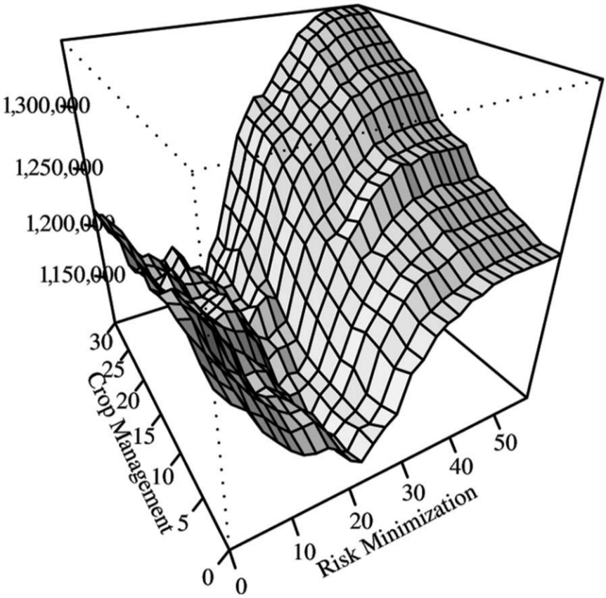
Variation in model fit as a function of risk minimization preference and crop management complexity preference weights.

Aggregate-Level Comparisons

For all crops, sign tests showed significant differences between model outputs and the Farm Business Survey results (the hypothesis x = c was rejected with p < 10⁻⁵ in all cases). This clearly demonstrates that for each of the crops, there is a bias in model predictions away from the observed values. The magnitude of these biases can be seen in Figure 3, which compares average crop areas (across all 149 farms) in the Farm Business Survey data and the model predictions.

Figure 3.

Comparison between the relative areas of the observed and simulated crops, showing a comparison (a) based on a pure-profit maximization model, (b) using outputs from a model using best-fit values of risk and crop complexity preferences, and (c) based on model outputs, including stated preference values for risk minimization and crop complexity.

Results are shown for the pure-profit model (Figure 3a), a model using the best-fit (minimum sum of squared differences) values for risk and crop complexity (Figure 3b), and a model with stated preference values for the risk and crop complexity parameters (Figure 3c). In each plot, a straight line indicates perfect agreement between modeled and observed data. Winter wheat is clearly the dominant crop but is always underpredicted by the model. In the pure-profit case (Figure 3a), the model severely overpredicts the area of potatoes and, to a lesser extent, overpredicts oilseed rape and bean crop areas. This fit is improved when farmer’s revealed and stated preferences for risk minimization are taken into account (Figures 3b and 3c). The main changes occur when risk preferences are applied. In particular, potatoes (which have high risk), and set-aside (which is low risk, with guaranteed subsidy income and near zero input cost), change rapidly as the risk preference is increased.

A Spearman rank test for correlation was not significant for the pure-profit model (Figure 3a; ρ = .53, p = .23) but was significant for the model including stated preferences (Figure 3c; ρ = .96, p = .003). The correlation for the model using revealed preferences (best-fit preferences from Figure 2) gave an intermediate correlation coefficient (Figure 3b; ρ = .75, p = .06). At first sight, this last result would seem to contradict the fact that the revealed preferences represent the minimum of sum of squared differences. However, as the Spearman rank test is based purely on rank order rather than minimizing squared differences, there is no inconsistency to be resolved.

Individual-Level Comparisons

Predicted (using stated preferences) and observed crop areas for seven types of land use on the 149 Farm Business Survey farms are compared in Figure 4. Visual inspection of this figure reveals that there is clearly a large amount of residual variation. The best predictions are obtained for winter wheat (the dominant crop) and for set-aside. Our statistical analysis (using the model described by Equation 7) revealed positive relationships between predicted and observed areas for most crops in Figure 4. The results of this regression are presented in Table 1 for four different models: (a) a purely empirical model that simply regressed crop gross margins against observed crop areas, (b) a pure-profit run of the model, (c) a run of the model using revealed preferences for risk and crop complexity (the best fits to the sum of squared deviations), and (d) a run of the model using stated preference values for risk and crop complexity. The overall ability of each model variant to explain variation in the observed cropping is summarized by the ΔDIC values (small values are better). Note that in the case of the stated preference model, the DIC was modified by 1 to account for the externally fitted parameter λ and was modified by 3 for the revealed preference model to account for fitted risk and crop complexity as well as λ. The stated preference model is clearly the best on this criterion, followed by the revealed preference model, and then the pure-profit model. The purely empirical benchmark model shows the worst fit.

Figure 4.

A direct comparison between relative crop areas simulated using the model with stated preferences and actual cropping for the 149 lowland arable farms selected from the 2000 to 2004 Farm Business Survey.

Table 1.

Fitted Values of the Slope Parameter β (for Each Crop) for Three Alternative Models of Crop Choice.

	Gross margin only β × 10⁻²	Pure-profit β × 10⁻²	Stated preferences β × 10⁻²	Revealed preferences β × 10⁻²
ΔDIC	34.1	12.9	11.1	0
Winter wheat	8.5 (1.6)	3.8 (0.8)	5.4 (1.7)	2.0 (0.8)
Winter oilseed rape	5.3 (2.3)	6.9 (2.0)	3.7 (2.3)	6.2 (2.1)
Potatoes	8.5 (3.2)	16 (6.4)	14.6 (16)	18 (8)
Legumes	3.0 (3.7)	13 (4)	10.6 (5.3)	13 (4)
Set-aside	9.9 (3.5)	7.8 (3)	6.7 (2.3)	9.7 (2)
Winter barley	5.2 (2.4)	8.5 (4)	24.2 (5.2)	17 (4)
Spring barley	−2.7 (3.7)	7.9 (6.3)	59.4 (21.7)	13 (8)

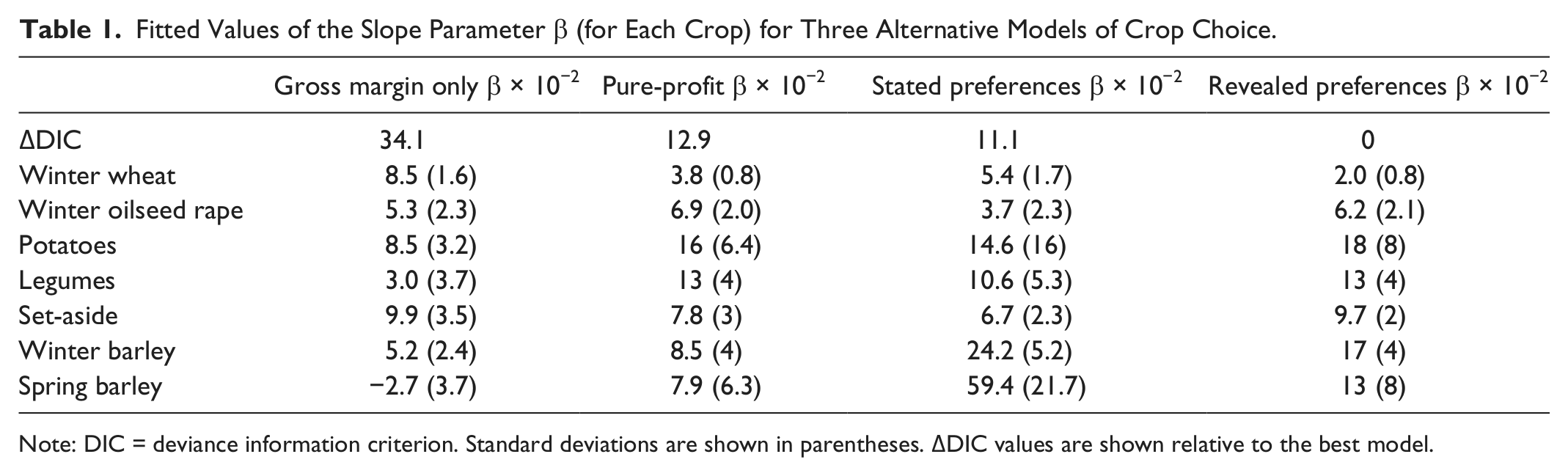
Note: DIC = deviance information criterion. Standard deviations are shown in parentheses. ΔDIC values are shown relative to the best model.

Discussion

In this article, we conducted a detailed statistical comparison between the outputs of a farm-level land-use model and observed cropping decisions over a 5-year period (2000-2004). Two main findings are presented. The first is that model results are essentially uncorrelated with actual farmer behavior, unless the model is modified to include farmer preferences other than pure profit (in our case, risk aversion and crop management complexity). Our second finding is that stated preference results can be used to parameterize models of farmer behavior, quantifying preference for risk aversion and potentially other preferences that might influence crop management decisions.

The question of whether multiple farm preferences (especially risk aversion) are a required component of predictive land-use models has been studied for many years. For example, Lin, Dean, and Moore (1974) reached the conclusion that profit-only models were inadequate based on a small sample of 6 farms, and more recently Rounsevell et al. (2003) found that farmers were approximately profit maximizers. Nevertheless, despite the long history of work examining this question, it remains unresolved (Just & Pope, 2003), partly because the sample sizes of some previous studies have been too small to analyze statistically (see, for example, Arriaza & Gómez-Limón, 2003; Lin et al., 1974), and because risk aversion is not likely to be important in all farming contexts (Edwards-Jones, Dreary, & Willcock, 1998). It is therefore unlikely that any single study will completely resolve the issue. Rather, a series of studies such as ours, which statistically compare model outputs with observed farmer behavior, and which use a large sample size (149 farms) are needed to examine the validity of modeling approaches in specific contexts.

There is a considerable body of work describing models for predicting the behavior of arable farmers in the United Kingdom and for closely related farming systems in continental Europe. A particularly relevant example is the work of Rounsevell et al. (2003), who used a similar profit model to ours, and conducted a quasi validation using a large number of sample points across East Anglia. Based on a comparison of crop areas for wheat, grass, and cereals, Rounsevell et al. found support for a profit-only model, but suggested that factors such as risk might also be important (though this was not tested). As our conclusions are somewhat at odds with the results of this article, it is worth explaining the difference. In our case, we conducted statistics on the basis of crop choice across a wide range of crops (8), and effectively tested the model’s ability to predict choices based on known yields and prices (inputs in our case). In contrast, Rounsevell et al. attempted to predict yields (using a formula based on soil type) but concentrated on the model’s ability to predict major crops. The difference between our results and those of Rounsevell et al. is interesting because they suggest that farmers’ choices may be more consistent with profit maximization when choosing among major crops, but that risk and other factors may influence those choices when minor crops and break crops are considered. Although small in total area, minor land uses such as set-aside or spring crops can be very important when modeling environmental issues.

We used a mixed-integer programming model to represent the profit, risk, and crop complexity functions of farmers in our study. Models of this type have a long history in agricultural modeling and many such models remain in use as policy tools (Arfini, 2005). The important alternative of PMP (de Frahan, 2005; Howitt, 1995) involves construction of a simplified profit function to which a correction is found such that the model can exactly reproduce a training data set. The advantage of this approach is that any aspect of the system that is relatively static does not need explicit description but instead can be subsumed into the correction function. Although this approach has proven to be very useful for policy prediction, it typically subsumes many aspects of farmer behavior, including risk aversion and crop complexity preference into the correction function. This is a problem if the goal of the study is to predict behavior under circumstances substantially different from the training data. It is therefore important that research into more explicit models continues alongside development of PMP. In particular, our study chose an explicit modeling approach rather than PMP because our goal was to explicitly test the importance of including behavioral functions in the model and to provide a means for their parameterization via interviews.

One of the principal practical difficulties with multiobjective behavioral models is that the relative weights of different objectives are difficult to quantify. In our study, we obtained these objective weights independently using detailed interviews with a sample of 49 farmers. Although interviews and stated preference surveys of farmers have often found support for land-use objectives other than profit (Gasson, 1973; McGregor et al., 1996; Perkin & Rehman, 1994), our study is unique in its ability to transfer these stated preferences directly into a land-use model. The main advantage of using stated preferences to parameterize a model is that they can be obtained relatively easily and independently of the land-use data used to test the model. The disadvantage is that it is difficult to elicit numerically accurate statements from interview participants without introducing well-known biases (Pöyhönen, Vrolijk, & Hämäläinen, 2001; Weber & Borcherding, 1993). For two key land-use objectives, risk preference and crop complexity preference, we obtained values corresponding to a best fit between our model and farmer behavior (in the form of land-use data). We found that the agreement between these best-fit values and stated values was much better for risk aversion than for crop complexity preference. As we used average satisfaction curves for both these objectives in our model, this disparity may be due to differences in the variance of satisfaction curves for each objective. It is difficult to reduce variance satisfaction curves to a simple numeric measure, but at a semiquantitative level, it is clear that risk (45/47 farmers with monotonic decreasing curves) was much less variable than crop complexity (31% decreasing, 50% humped, and 19% increasing). The fact that we condensed this variability into an average set of objective curves to be used across all farmers is not ideal, especially for the crop complexity parameter. In future work, we would like to collect land-use data for the 49 farmers interviewed rather than rely on existing land-use databases that provide data for different farmers.

Tight integration in this study between model building and the design of preference elicitation interviews was essential for developing a well-parameterized socioeconomic model. In addition to providing parameters, the stated preference survey was used to screen objectives for inclusion in the model based on the relative importance to farmers and relative influence on crop-choice variability. As model complexity rapidly increases with the inclusion of additional objectives, this latter step is crucial to successful model development. However, it is possible that further improvements to the accuracy of arable landscape models could be achieved through the inclusion of additional objectives such as landscape structure, wildlife, and nonproduction land use. The key to the success of such work, however, will be the joint collection of detailed financial, physical, and preference information at the individual farm level. Such information will be essential to reduce noise due to parameter error and allow the relative performance of different models to be assessed.

Footnotes

Appendix A

Appendix B

Authors’ Note

This work was conducted as part of the Research Councils’ Rural Economy and Land Use (RELU) program.

Declaration of Conflicting Interests

The author(s) declared no potential conflicts of interest with respect to the research, authorship, and/or publication of this article.

Funding

The author(s) disclosed receipt of the following financial support for the research and/or authorship of this article: Rural Economy and Land Use (RELU) is funded jointly by the Economic and Social Research Council, the Biotechnology and Biological Sciences Research Council, and the Natural Environment Research Council, with additional funding from the Department for Environment, Food and Rural Affairs and the Scottish Executive Environment and Rural Affairs Department. W.J.S. is funded by Arcadia.

Author Biographies

Ira R. Cooke is currently a research scientist with the Life Sciences Computation Centre at La Trobe University, Australia. He has applied computational and statistical techniques to answering a broad range of life science questions ranging from landscape ecology to subcellular processes.

Elizabeth H. A. Mattison is a postdoctoral research assistant whose work explores land managers’ beliefs and intentions and their effects on associated biodiversity. She has worked in a variety of agricultural and wildlife management contexts developing predictive models of biodiversity outcomes.

Eric Audsley is a principal research fellow at Cranfield University. Before that, he worked for 34 years at Silsoe Research Institute, formerly the U.K. Agricultural Research Council’s National Institute of Agricultural Engineering, until its closure in 2005. He has developed the application of mathematical and operational research techniques to the analysis of decisions concerning a very wide range of agricultural systems. Currently major areas are linear programming modeling of farms to predict future agricultural land use and model-based environmental Life Cycle Inventory Analysis (LCA) of agricultural production systems.

Alison P. Bailey is a senior lecturer in agricultural business management at the University of Reading. Her research focuses on the analysis of agricultural production systems and the relationship between agriculture, the environment, and socioeconomic criteria. This includes assessment of farmer decision-making processes and motivations associated with farming practice.

Robert P. Freckleton is a professor of population biology at the University of Sheffield. He works on the application of ecological and evolutionary models to understand the effects of environmental change on ecological systems.

Anil Graves is a Senior Research Fellow in Land Use Systems and applies his background in the natural and social sciences to investigating land use problems. Initially he spent several years in India researching the hydrological and social impacts of reforestation, coastal saline intrusion, and groundwater abstraction. Since returning to the UK, he has worked on a range of UK and EU projects, researching the biophysical, economic, and social aspects of arable, forestry, and agroforestry systems in Europe, and more recently, on the application of the ecosystem framework.

Joe Morris is emeritus professor in resource economics and management in the School of Applied Sciences, Cranfield University, Bedford, England. His recent work has focused on the sustainable management of agriculture and natural resources with particular reference to the economics of land, water, and ecosystems.

Simon A. Queenborough is currently a senior research associate at The Ohio State University, USA. He is interested in mechanisms of species coexistence, and the evolutionary and ecological effects of variation in breeding systems and patterns of resource allocation.

Daniel L. Sandars is a research fellow in operational research in natural resource management at Cranfield University’s School of Applied Sciences and formerly at the Silsoe Research Institute’s Biomathematics, and Mathematics and Decisions Systems groups.

Gavin M. Siriwardena is head of Land-Use Research at the British Trust for Ornithology. He works primarily on bird ecology in farmland and other terrestrial habitats, with a particular focus on population responses to management and habitat characteristics.

Paul Trawick is the chair of the Department of Sociocultural Anthropology at Idaho State University. His research interests focus on the management of water for irrigation, viewing the problem as a social rather than a technological one. By comparing successful irrigation systems in different parts of the world, he has identified the institutions and operating principles for sharing a scarce water resource.

Andrew R. Watkinson is executive director of the Living With Environmental Change partnership and a professorial fellow at the University of East Anglia. He was formerly director of the Tyndall Centre for Climate Change Research. He is interested in the application of population biology in farming systems and the impacts of environmental change on the coastal zone.

William J. Sutherland holds the Miriam Rothschild Chair in conservation biology at the University of Cambridge. He is interested in predictive models of ecological systems, improving the effectiveness of the use of science in policy and in evidence-based conservation.

References

Agro Business Consultants. (2004). The agricultural budgeting and costings book (59th ed.). Melton Mowbray, UK: Author.

Annetts

J. E.

Audsley

(2002). Multiple objective linear programming for environmental farm planning. Journal of the Operational Research Society, 53, 933-943.

Arfini

(2005). Modelling agricultural policies: State of the art and new challenges. Proceedings of the 89th Seminar of the European Association of Agricultural Economists, University of Parma, Italy.

Arriaza

Gómez-Limón

J. A.

(2003). Comparative performance of selected mathematical programming models. Agricultural Systems, 77, 155-171.

Beale

E. M. L.

Forrest

J. J. H.

(1976). Global optimization using special ordered sets. Mathematical Programming, 10, 52-69.

Belton

Stewart

T. J.

(2002). Multiple criteria decision analysis: An integrated approach. Dordrecht, Netherlands: Kluwer Academic.

Brodt

Klonsky

Tourte

(2006). Farmers’ goals and management styles: Implications for advancing biologically based agriculture. Agricultural Systems, 89, 90-105.

Cowles

M. K.

Carlin

B. P.

(1996). Markov Chain Monte Carlo convergence diagnostics: A comparative review. Journal of the American Statistical Association, 91, 883-904.

de Frahan

B. H.

(2005, August). PMP Extensions and alternative methods: Introductory review of the state of the art. XIth European Association of Agricultural Economists Congress, Copenhagen, Denmark.

10.

Department for Environment, Food and Rural Affairs. (2008). Agriculture in the United Kingdom. Retrieved from http://www.defra.gov.uk/statistics/files/defra-stats-foodfarm-farmgate-api-2005-130321.xls

11.

Department for Environment, Food and Rural Affairs & National Assembly for Wales. (2002). Farm Business Survey. Colchester, Essex: UK Data Archive (SN: 4604).

12.

Department for Environment, Food and Rural Affairs & National Assembly for Wales. (2003). Farm Business Survey. Colchester, Essex: UK Data Archive (SN: 4830).

13.

Department for Environment, Food and Rural Affairs & National Assembly for Wales. (2004). Farm Business Survey. Colchester, Essex: UK Data Archive (SN: 4831).

14.

Department for Environment, Food and Rural Affairs & National Assembly for Wales. (2005). Farm Business Survey. Colchester, Essex: UK Data Archive (SN: 5228).

15.

Edwards-Jones

Dreary

Willcock

(1998). Incorporating psychological variables in models of farmer behaviour: Does it make for better predictions? Etudes & Recherches sur les Systèmes Agraires et le Développement, 31, 153-173.

16.

Fairweather

J. R.

Keating

N. C.

(1994). Goals and management styles of New Zealand farmers. Agricultural Systems, 44, 181-200.

17.

Gasson

(1973). Goals and values of farmers. Journal of Agricultural Economics, 24, 521-542.

18.

Gelman

Carlin

J. B.

Stern

H. S.

Rubin

D. B.

(2002). Bayesian data analysis (2nd ed.). Boca Raton, FL: Chapman and Hall/CRC.

19.

Geweke

(1992). Evaluating the accuracy of sampling-based approaches to the calculation of posterior moments. In Bernardo

J. M.

Berger

David

A. P.

Smith

A. F. M.

(Eds.), Bayesian statistics 4 (pp. 169-193). Oxford, UK: Oxford University Press.

20.

Harper

W. M.

Eastman

(1980). An evaluation of goals hierarchies for small farm operators. American Journal of Agricultural Economics, 62, 742-747.

21.

Hazell

P. B. R.

(1971). A linear alternative to quadratic and semivariance programming for farm planning under uncertainty. American Journal of Agricultural Economics, 53, 53-62.

22.

Howitt

R. E.

(1995). Positive mathematical programming. American Journal of Agricultural Economics, 77, 329-342.

23.

Janssen

van Ittersum

M. K.

(2007). Assessing farm innovations and responses to policies: A review of bio-economic farm models. Agricultural Systems, 94, 622-636.

24.

Just

R. E.

Pope

R. D.

(2003). Agricultural risk analysis: Adequacy of models, data, and issues. American Journal of Agricultural Economics, 85, 1249-1256.

25.

Lin

Dean

Moore

C. V.

(1974). Profit maximization in agricultural production. American Journal of Agricultural Economics, 56, 497-508.

26.

McGregor

Willock

Dent

Deary

Sutherland

Gibson

. . . Grieve

(1996). Links between psychological factors and farmer decision making. Farm Management, 9, 228-239.

27.

Ministry of Agriculture, Fisheries and Food & National Assembly for Wales. (2001). Farm Business Survey. Colchester, Essex: UK Data Archive (SN: 4603).

28.

Moffett

Dyer

J. S.

Sarkar

(2006). Integrating biodiversity representation with multiple criteria in North-Central Namibia using non-dominated alternatives and a modified analytic hierarchy process. Biological Conservation, 129, 181-191.

29.

Mustajoki

Hämäläinen

R. P.

Salo

(2005). Decision support by interval SMART/SWING – incorporating imprecision in the SMART and SWING methods. Decision Sciences, 36, 317-339.

30.

Nix

(2007). Farm management pocketbook (37th ed.). Leicestershire, UK: The Andersons Centre.

31.

Pacini

Wossink

Geisen

Huirne

(2004). Ecological-economic modeling to support multi-objective policy making: A farming systems approach implemented for Tuscany. Agriculture, Ecosystems and Environment, 102, 349-364.

32.

Perez

Muller-Holm

(2001). Economic incentives and technological options to global warming emission abatement in European Agriculture. In Arfini

(Ed.), Modelling agricultural policies: State of the art and new challenges: Proceedings of the 89th Seminar of the European Association of Agricultural Economists (pp. 413-425). Parma, Italy: University of Parma.

33.

Perkin

Rehman

(1994). Farmers’ objectives and their interactions with business and life styles: Evidences from Berkshire, England. In Dent

J. B.

McGregor

M. J.

(Eds.), Rural and farming systems analysis: European perspectives (pp. 193-212). Wallingford, UK: CAB International.

34.

Plummer

Best

Cowles

Vines

(2006). CODA: Convergence diagnosis and output analysis for MCMC. R News, 6, 7-11.

35.

Pöyhönen

Vrolijk

H. C. J.

Hämäläinen

R. P.

(2001). Behavioral and procedural consequences of structural variation in value trees. European Journal of Operational Research, 134, 218-227.

36.

Press

W. H.

Teukolsky

S. A.

Vetterling

W. T.

Flannery

B. P.

(1992). Numerical Recipes in Fortran 77 (2nd ed.). New York, NY: Cambridge University: Press.

37.

R Development Core Team. (2008). R: A language and environment for statistical computing . Vienna, Austria: R Foundation for Statistical Computing. Available from http://www.R-project.org

38.

Rounsevell

M. D. A.

Annetts

J. E.

Audsley

Mayr

Reginster

(2003). Modelling the spatial distribution of agricultural land use at the regional scale. Agriculture, Ecosystems and Environment, 95, 465-479.

39.

Seo

S. N.

Mendelsohn

(2008). An analysis of crop choice: Adapting to climate change in South American farms. Ecological Economics, 67, 109-116.

40.

Solano

Léon

Pérez

Herrero

(2001). Characterising objective profiles of Costa Rican dairy farmers. Agricultural Systems, 67, 153-179.

41.

Spiegelhalter

D. J.

Best

N. G.

Carlin

B. P.

van der Linde

(2002). Bayesian measures of model complexity and fit. Journal of the Royal Statistical Society: Series B, 64, 583-639.

42.

von Winterfeldt

Edwards

(1986). Decision analysis and behavioral research. Cambridge: Cambridge University Press.

43.

Watkinson

A. R.

Freckleton

R. P.

Robinson

R. A.

Sutherland

W. J.

(2000). Predictions of biodiversity response to genetically modified herbicide-tolerant crops. Science, 289, 1554-1557.

44.

Weber

Borcherding

(1993). Behavioral influences on weight judgments in multi-attribute decision making. European Journal of Operational Research, 67, 1-12.

Empirical Test of an Agricultural Landscape Model

Abstract

Keywords

Introduction

Trading-Off Multiple Objectives: Mathematical Framework

Estimation of Preferences

Choice of Objectives and Calculation of Weights

Satisfaction Curves

Model Components for Specific Objectives

Profit Objective

Risk Minimization Objective

Statistical Methodology for Comparing Land-Use Data With Model Outputs

Empirical Data Used

Model Runs

Measuring Model Fit

Results

Best-Fit Estimates for Risk and Crop Complexity Preferences

Aggregate-Level Comparisons

Individual-Level Comparisons

Discussion

Footnotes

Appendix A

Appendix B

Authors’ Note

Declaration of Conflicting Interests

Funding

Author Biographies

References