Sage Journals: Discover world-class research

Abstract

Expressive music performance and cardiac arrhythmia can be viewed as deformations of, or deviations from, an underlying pulse stream. I propose that the results of these pulse displacements can be treated as actual rhythms and represented accurately via a literal application of common music notation, which encodes proportional relations among duration categories, and figural and metric groupings. I apply the theory to recorded music containing extreme timing deviations and to electrocardiographic (ECG) recordings of cardiac arrhythmias. The rhythm transcriptions are based on rigorous computer-assisted quantitative measurements of onset timings and durations. The root-mean-square error ranges for the rhythm transcriptions were (19.1, 87.4) ms for the music samples and (24.8, 53.0) ms for the arrhythmia examples. For the performed music, the representation makes concrete the gap between the score and performance. For the arrhythmia ECGs, the transcriptions show rhythmic patterns evolving through time, progressions which are obscured by predominant individual beat morphology- and frequency-based representations. To make tangible the similarities between cardiac and music rhythms, I match the heart rhythms to music with similar rhythms to form assemblage pieces. The use of music notation leads to representations that enable formal comparisons and automated as well as human-readable analysis of the time structures of performed music and of arrhythmia ECG sequences beyond what is currently possible.

Keywords

Atrial fibrillation cardiac arrhythmia expressive music performance free rhythms irregular pulse meter music notation music representation timing

Introduction

Expressive music performance and cardiac arrhythmia share many common traits. An important one is that each can be viewed as the result of deviations from, or deformations of, an underlying pulse. Their origins suggest that the rhythms of such data streams can be encoded effectively using common music notation. I propose to treat these time displacements as bona fide rhythms and to represent them via a literal application of music notation. Music notation encodes abstract concepts of proportional relations among duration categories, and higher-level organizing constructs such as figural and metric groupings, and is typically used for abstract or conceptual, rather than literal, representations of time. The literal application (and consequent reading) of common music notation is counter to its common use by composers or performers. I co-opt the existing notation system to create symbolic representations that can enable formal comparisons and computer and human analysis of time sequences.

This work was inspired by a transcription of sight-reading wherein the rhythm notation captured both musical and cognitive disfluencies. The transcription, created by ear with the aid of the original score and audio and Musical Instrument Digital Interface (MIDI) recordings, demonstrated the possibility of notating serendipitous rhythms. In this article, I will use computer tools to rigorously mark onset times and obtain quantitative measurements of durations. The tempi and quantizations are chosen to maximize transcription precision, and the accuracies of the rhythm transcriptions are evaluated quantitatively against the original timings. Figural and metric groupings and any metric modulations are chosen manually, although this too can be automated, as will be discussed.

The technique is first illustrated using contrasting music examples that contain extreme timing deviations introduced in performance. The results highlight the gap between the score and performance, made all the more obvious by the use of the same notation to communicate the difference between the rhythms. Next, I apply the same transcription process to electrocardiographic (ECG) recordings of cardiac arrhythmias. While such rhythm transcription can be applied to any arrhythmia, I demonstrate the method on three excerpts of ECG recordings of atrial fibrillation. The notation shows clearly the rhythmic groupings and patterns such as repetitions and transformations through time. These are patterns normally obscured in the predominant ECG analysis approaches, which mainly consider individual beat morphology or features aggregated over windows of time.

Similarities between cardiac and music rhythms are further made tangible by matching the heart rhythms to music with similar rhythms to form musical assemblages. I apply the notation and retrieval-and-assemblage process to the atrial fibrillation ECG recordings, leveraging the innate rhythmic similarities to music with mixed meters, a siciliane, and a tango to generate the mirror pieces.

The precise and symbolic representation of performers’ idiosyncratic timings and of atrial fibrillation’s capricious rhythms points to a host of new computational analysis approaches for characterizing and comparing such time sequences. Once a formal representation for time structure exists in symbolic form, any number of encoding schemes can be employed to transform the symbols to machine-readable formats. These encoding schemes facilitate fast searches for specific rhythms and repeated patterns, allowing for data summarization and comparisons between sequences. Further analyses of the transcribed rhythms could reveal hierarchical structure in the time series data. Quantitative techniques can be devised to measure the distance, for example, between transcriptions of different performances of the same work. Finally, the symbolic representation lends itself to large-scale pattern search and categorization, for inferring performance style, characterizing arrhythmia subtypes, or predicting diagnostic outcomes.

The remainder of the article is organized as follows: first I review some related work on transcription, music performance, and mappings of cardiac information to music; next, I briefly review the sight-reading transcription that inspired this work; then, I present the transcriptions of the three performed music cases, followed by the three arrhythmia ECG transcriptions, and conclusions and discussions. An appendix documents the evaluations of the various transcriptions.

Transcription

The practice of transcription has an illustrious history. Olivier Messiaen’s (1956) use of birdsong in his compositions, such as Oiseaux Exotique, Vingt Regards, and others, is well known. The tradition of transcribing birdsong pre-dates Messiaen by many centuries. Hold (1970) gives a detailed account of composers’ and naturalists’ attempts at music representations of birdsong from 1240 onwards—these include staff, orthochronic, and graph notation, and the sound spectrograph.

Transcription has been especially useful for the study and reproduction of extemporaneous performances. Early examples can be found in Vaclav Pichl’s transcriptions of Luigi Marchesi’s (1792) elaborate note embellishments in four performances of the aria “Cara negl’occhi tuoi” and the rondo “Mi dà consiglio” in Nicola Antonio Zingarelli’s opera Pirrore d’Epiro, as described in Berger (2016). The Charlie Parker Omnibook (1978), a collection of transcriptions of the jazz saxophonist’s compositions and improvised solos, remains a staple in jazz studies. Historic performances like Keith Jarrett’s Köln Concert (1975) have been painstakingly notated for re-performance. Other transcriptions include those of Coltrane (1999), Duke Ellington (1971), Bill Evans (1967), and Ferdinand “Jelly Roll” Morton (1986), as reviewed in Tucker (1982).

Ethnomusicologists and composers transcribe field recordings of folk songs for analysis and as seed material for new compositions, respectively. Béla Bartók (1942) carefully converted to music notation the melodies of recorded songs in the Milman Parry Collection for re-use in compositions; see the discussion in Frigyesi (1985).

More recently, the push toward an empirical study of vernacular music has led to the transcription of traditional Chinese clapper music and rap music for systematic analysis; see Sborgi Lawson (2012) and Ohriner (2016), respectively.

This work was motivated in part by Practicing Haydn (Grønli, Child, & Chew, 2013), in which a sight-reading of a Haydn sonata movement is transformed into a performable score via transcription, complete with all the repetitions, pauses, starts, and stops. The transcription of sight-reading raises the following question: If the blundering mishaps and accidental discontinuities of a first encounter with a score can be recorded using music notation, what else might be amenable to such treatment? Here, we show that expressive performance and arrhythmia sequences can also be subject to such transcription processes, although the goal is not to produce a performable score, even though that is a desirable side effect, and the transcription will use a computer-assisted process that aims to minimize discrepancies between original and transcribed sequences.

Related to transcription of expressive performance, there exists a long tradition of scholarly work on the representation of intonation, dynamics, and pacing in expressive speech, dating back to Steele (1775). Recent forays into the transcription of speech melody and timing have turned to the direct use of music notation in a literal fashion. Leveraging commonalities between expressive speech and music, Simões and Meireles (2016) and Meireles, Simões, Ribeiro, and de Medeiros (2017) explored the use of music notation to represent the melody and rhythms of spoken language. In this work, the transcriptions are treated as literal expressions of the spoken pitches and durations. They are uniformly presented in 4/4 time, without regard to meter, although the authors propose that they will obtain natural metrical groupings from the stresses in speech in future work.

This article applies music transcription to unconventional contexts of expressive performance and cardiac arrhythmia, with the goal of recording these temporal processes and experiences, which are not normally preserved in writing. Special attention will be given to precise representation of timing and durations, and to the figural and metrical groupings that may be inferred from the patterns.

Representing performed music

The first application addresses the representation of performed music. The increased emphasis on music as performance rather than music as writing or notation, combined with the growth of computer tools for analysis of performed music, brings to a head issues of representing performed music. Anyone who has tried to generate a sound file from a digital score soon discovers that a performance rendered from the digital score is vastly different from that realized in practice. Thus, the information encoded in the score is insufficient for creating or re-creating a convincing rendition of the music. This is because, as Frigyesi (1993, pp. 60–62) points out, notation was not conceived to be transcription; it represents only an abstraction of the temporal experience, and not the actual rhythms of a performance. It is worth noting that the view of transcription as literal and notation as abstract is not universal. For example, Busoni considers the transfer of a piece from one instrument to another, the transfer of music concept to notation (composition), and the transfer from notation to performance to be different forms of transcription, see Knyt (2010, p. 111). The transcriptions in this article will use notation literally to encode time and other structures.

Music as performed differs from the information denoted on the page for many reasons. In performed speech, the measure of syllables and words in a text fall far short of the timings of the delivery. In music playing that aspires to the rhetorical style of spoken language á la Adolph Kullak, see Cook (2013, p. 74), performed rhythms privilege the cadences and pacing of speech over the music script. Owing to the relative nature of loudness and other constraints, notated dynamics are also frequently not what they seem: Kosta, Bandtlow, and Chew (2014) showed that notes marked pianissimo can sound objectively louder than notes marked fortissimo, depending on context. Furthermore, music performance practice often requires that performers deviate from the written score in prescribed ways. For example, in the French tradition of notes inégales, notes of equal duration are deliberately lengthened or shortened in performance, see Houle (2000, p. 86). In many folk traditions, notated pitches may be lavishly ornamented in practice, as shown in a study of Yang, Chew, and Rajab (2013), which compares erhu and violin performances of a Chinese folk piece.

However, what if actual performed rhythms were transcribed literally and precisely using conventional notation so as to make the nuances of performance concrete through writing? The encoding would still be incomplete as the symbolic representation would not capture fine details, such as the exact shapes of note articulations, transitions, and within-note embellishments. Some degree of approximation of the precise timings will be inevitable to ensure the readability of the transcription; even if the transcription could provide notation to millisecond precision, there are limits to what the human ear can distinguish as two separate time instants, see Bartlette, Headlam, Bocko, and Velikic (2006), Chafe, Caceres, and Gurevich (2010), and Chew et al. (2004). Nonetheless, a faithful transcription would give a much more accurate (literal) representation of the temporal experience, and would allow for direct comparison with the original score as a measure of the distance between the abstract representation and actual experience.

Notation of and for performance has taken many forms. Philip (1992) has explored the notation of nuances in expressive timing in less quantitative ways. Moving away from conventional music notation, Bamberger’s (2000) Impromptu software uses a number of representations, such as pitch contours, rhythm bars, and piano roll notation to allow users to manipulate properties of tune blocks. Many other graphical notations exist, including those of Farbood (2004) and Hope and Vickery (2015). As an intermediary between conventional notation and digital sound, OpenMusic (Bresson & Assayag, 2011), a programming environment designed for composition and analysis, allows notes to be positioned on staff lines in continuous locations indicating the times at which they sound, with impact on the readability of the score. A goal here will be to explore the limits of using conventional music notation to represent continuous time, bearing in mind that not all locations on the continuous time axis are equally likely, given the pulse-based origin of the input.

The first set of examples takes on this challenge to transcribe the actual timings of recorded expressive performances. In so doing, it provides, in a sense, a written record of the performers’ creative work. The three cases span music from a variety of Western music traditions: the Vienna Philharmonic Orchestra’s performances of Johann Strauss II’s The Blue Danube, a traditional New Year’s concert encore piece; Maria Callas’ rendition of Giacomo Puccini’s operatic aria “O Mio Babbino Caro,” and Marilyn Monroe’s sultry rendition of “Happy Birthday” on the occasion of John F. Kennedy’s 45th birthday.

The body of scientific research on performance practice has expanded rapidly, aided by recent software tools, such as Sonic Visualiser by Cannam, Landone, and Sandler (2010). It is now possible for any motivated person with modest computer literacy to be able to extract beat and loudness information from a recorded performance. Because of the visual and compact nature of information portrayed on graphs, the scientific study of music performance and music expression predominantly uses graphs of timing, tempo, or loudness data extracted from audio recordings—see, for example, Todd (1992), Cheng and Chew (2008), and Chew (2016). There has scarcely been any attempt to notate these captured rhythms, owing partly to the gulf between event-based (notation) and signal-based (audio) representations, and partly to the difficulty of representing free rhythms, which will be discussed in upcoming paragraphs.

An exception can be found in the work of Beaudoin and Senn, described in Beaudoin and Kania (2012), in which the exact timings and intensity levels of Martha Argerich’s recording of Chopin’s “Prelude in E minor,” Op. 28/4, is transcribed in standard notation as the framework for a series of pieces based on transformations on Chopin’s original material called Études d’un Prélude. Another is the work of Grønli, Child, and Chew (2013), in which Chew’s sight-reading of the finale movement of Haydn’s Piano Sonata in E♭, Hob XVI:45 is meticulously transcribed by Child for re-performance. The resulting composition, Practicing Haydn, was created for and premiered at Grønli’s solo art show at the grand opening of the Kunsthall Stavanger, and at other venues.

Musica humana

The second application lies in the domain of cardiac arrhythmia. The belief that music is inherent in the beating of the pulse was widely held in the Middle Ages. This was a specific instance of the more general idea that music is inherent in the rhythms of the human body—Boethius’ Musica humana, which is complementary to Musica instrumentalis (music of sounding instruments) and Musica universalis (music of the spheres), see Chamberlain (1970). Siraisi (1975) provides a rich survey of academic physicians’ detailed writings on the nature of the music of pulse in the 14th and 15th centuries. Since then, arts and medicine have diverged and developed along separate paths. Today, with the parallel development of annotation and visualization tools like WFDB by Silva and Moody (2014) and LightWAVE by Moody (2013) for ECG data, there is ample evidence that the human pulse would be amenable to modern musical treatment and analysis, as the fields are poised to collide again.

As a step toward facilitating this reconnection, the second set of examples applies transcription to represent, using conventional music notation, the rhythms of arrhythmia. Music representation of cardiac information is not new, although it has been used primarily to describe heart sounds. Renà Laennec (1826), the inventor of the stethoscope, used mainly onomatopoeic words to depict sounds he heard in the process of auscultation; however, on one occasion in 1824, he resorted to music notation to augment his word description of a venous hum. Segall (1962) points to this as the first symbolic representation of the sound of a heart murmur, with many more graphical notations to follow. More recently, Field (2010) used music notation to systematically transcribe signature heart sounds and murmur patterns in the teaching of cardiac auscultation to medical students to aid the diagnosis of heart valve disorders.

I will also use music notation to represent heart rhythms, but now focusing on the transcription of recorded rhythmic sequences of abnormal electrical activity in the heart. Conditions resulting from abnormal electrical conduction differ from those due to valvular disorders; the input will also be the ECG trace instead of sound.

Conventional ways to represent ECG data tend to focus on individual beats: their morphology (features of the waveform) or categorical labels, such as N (normal) and V (ventricular activity); or, frequency-domain characteristics like heart rate variability that aggregate features over larger windows of time. Counter to this trend, Bettermann, Amponsah, Cysarz, and van Leeuwen (1999) used a binary symbol sequence from African music theory to represent elementary rhythm patterns in heart period tachograms. Syed, Stultz, Kellis, Indyk, and Guttag (2010) consider motific patterns based on short strings of the categorical labels, and Qiu, Li, Hong, and Li (2016) have studied the semantic structure of symbols labeling parts of the waveform.

In the context of the transcription exercise, the notated rhythms are next matched to existing music with similar rhythms, and new compositions generated by collaging together appropriate parts of the selected piece. Since the chosen music already has the same or a very similar rhythmic structure, the collage gives pitch to the rhythms in ways that reinforce and make more readily perceptible the inherent time structures. If the pitch structures are in dialog with the time structures, the collage can add a layer of complementary structures. In either case, the temporal experience of arrhythmia can be made visceral through the performance of the resulting music.

Composing with rhythm templates is not new. Composer Cheryl Frances-Hoad’s piano piece Stolen Rhythm (2009) takes the notated rhythms of the finale movement in Haydn’s Piano Sonata in E♭, Hob XVI:45, and assigns new pitches to them. The computer program MorpheuS also takes rhythms from existing pieces and sets new notes to them in ways that preserve the repetition patterns, and tonal tension profiles of the template piece, see Herremans and Chew (2017). Practicing Haydn, in effect, creates a collage by traversing Haydn’s piece through a series of repetitions and pauses.

Heartbeat data have been used as a source for music composition or synthesis. The most common approach is to use heart rate variability indices, which are based on statistical aggregation over longer time spans. There is also a tendency toward direct data sonification. In the Heartsongs CD by Davids (1995), produced as part of ReyLab’s Heartsongs Project, heartbeat intervals were averaged over 300 beats to remove local fluctuations and mapped to 18 notes on a diatonic scale to create a melody. Yokohama (2002) maps each heartbeat interval to MIDI notes, so that an intervallic change such as a premature beat triggers a more significant change in pitch. In Ballora, Pennycook, Ivanov, Glass, and Goldberger (2006), heart rate variability data is mapped to pitch, timbre, and pulses over a course of hours for medical diagnosis; in Orzessek and Falkner (2006), heartbeat intervals are passed through a bandpass filter and mapped to MIDI note onsets, pitch, or loudness. The Heart Chamber Orchestra (Votava & Berger, 2011) uses interpretations of its 12 musicians’ heartbeats, detected through ECG monitors; relationships between them influence a real-time score that is then read and performed by the musicians from a computer screen. All but one of these studies—Yokohama (2002)—have focused on heartbeat data from non-arrhythmic hearts.

In this article, transcription serves as a means to represent the rhythms of arrhythmia using conventional music notation. Current analyses of ECG data predominantly use representations based on beat morphology and representations in the frequency domain. The music notation captures local rhythmic patterns that are lost in single-beat and frequency-based approaches. Three different excerpts, short summaries, showing a heart in different states of atrial fibrillation are chosen from a continuous 18-hour recording from a three-lead Holter monitor. The rhythms of the different states of the arrhythmia are made apparent in the extracted musical rhythms and collage pieces.

Transcription process

Conventional music notation is the representation of choice for the transcriptions in this article. The examples addressed in this article tend toward the practice of free rhythm, which is common in both folk and art, religious and secular traditions. Free rhythm is “the rhythm of music without pulse-based periodic organization” Clayton (1996, p. 329). The analysis of free-rhythm music remains an open challenge, with a major hurdle being the difficulty of representing free rhythms in writing. Existing efforts to notate free rhythms typically avoid time signatures or bar lines, sometimes simply arranging note heads on a horizontal timeline so as to avoid the implications of pulse or meter in staff notation.

The reason regular staff notation is adopted here is that the examples are all pulse-based; this includes both the performed music as well as the cardiac arrhythmia time series. While they generally lack periodic structure and do not possess ordinary metrical organization, owing to pauses and pattern repetitions, local grouping structures do emerge, which allow for the assignment of changing time signatures and indications of figural groupings through note beaming or phrase markings. In line with notations used in contemporary compositions, the transcription of Practicing Haydn, and indeed those for the performed durations and arrhythmia sequences make copious use of changing meters (as in Stravinsky’s compositions), and metric modulations (as in Elliot Carter’s works).

A main objective in the transcription process is to minimize the difference between the recorded and the transcribed sequence. When a design goal is to minimize transcription error, there exists the possibility of making the notation enormously complex to achieve the highest possible accuracy. To counter this, an important and competing aim is to ensure that the proportional durations in the notation are readily readable by human eyes, so that the transcription could serve as a source for visual analysis or performance. In this way, the notation is suitable as input for computer analysis as well as for visual inspection. Metric modulations are kept to a minimum, and utilized only when they lead to simpler proportional durations. To satisfy the second goal, when a human performer plays the notated transcription, it should be possible to reproduce the original rhythms without the aid of a click track, as in https://vimeo.com/226516952, although clearly it would be easy to choose to deviate significantly from the score. Thus, the labyrinthine density of notation like that employed by Brian Ferneyhough as a conduit for his complex composition process is avoided in favor of simpler forms. In the case of Ferneyhough’s intricate notation, designed to serve the purpose of lifting players beyond hackneyed readings of the score, some, such as Marsh (1994), have argued for simpler representations that directly reflect specific interpretations of the music. Distinct from Marsh’s goals, even though a secondary constraint of the transcription process here is human readability, the transcriptions do tend to make the score more complex in order to incorporate recorded nuances. Here, metric modulations that use irrational proportions, as in Conlon Nancarrow’s Study 33, are strictly avoided. One might argue that even Nancarrow’s irrational proportions can be closely approximated using conventional notation (rational durations) for playability, see Callender (2014).

Rhythmic disfluencies

The transcription of performed rhythms and the rhythms of cardiac arrhythmias draws inspiration from Practicing Haydn by Chew, Child, and Grønli (2013). Practicing Haydn originated as an idea by Grønli and Child to create a musical piece that sounds like musicians warming up and practicing before a concert. The result was a transcription of the serendipitous rhythms of a sight-reading of a Haydn sonata movement for re-performance, complete with all the repetitions, starts, and stops. The premiére of the piece took place concurrently at the grand opening of the Kunsthall Stavanger in Norway by Chew and at Performa13 in New York City by pianist Elaine Kang—see videos at https://kunsthallstavanger.no/en/exhibitions/practicing-haydn.

Three selections from the transcription are given in Figures 1 to 3. Each figure shows a snippet from the original Haydn score and a snippet from Child’s transcription of Chew’s sight-reading of the corresponding bars. The transcribed segments are inevitably longer than the original score, owing to repetitions, and to pauses and hesitations.

Figure 1.

Chew’s sight-reading of Haydn’s Piano Sonata in E♭, Hob XVI:45 finale: pauses and repetitions.

Figure 2.

Chew’s sight-reading of Haydn’s Piano Sonata in E♭, Hob XVI:45 finale: slow-downs, repetitions, and hesitations.

Figure 3.

Chew’s sight-reading of Haydn’s Piano Sonata in E♭, Hob XVI:45 finale: repetitions and wrong note.

An interesting side effect of the exercise is that the transcription serves as a record of not only the musical but also the cognitive disfluencies. Unexpected events provide moments for pause. The transcribed sight-reading in Figure 1(b) shows a pause at the end of the second bar just before an unfamiliar turn in the 16th-note sequence; the excerpt in Figure 2(b) documents the hesitations just before the introduction of figural or directional changes; the pickup into the 2/4 bar re-starts an unexpected figure that was not fully apprehended on the first play in the preceding 3/8 bar; a similar re-start can be observed in Figure 3(b). Repetitions help refine harmonic direction: in Figure 1(b) the trill is repeated to reinforce its harmonic function; in Figure 2(b), the final tonic chord is elongated to balance the length (and emphasis) of the preceding dominant chord.

That sight-reading is associated with hesitation and fumbling is not particularly remarkable. What is interesting here is that these behaviors are clearly documented in the transcriptions. They may be obvious to a casual listener, but the fact that they show up clearly in the transcriptions means that it is possible to automate the detection process to enable large-scale analysis of disfluent or rhythmically irregular behavior.

Choreographed rhythms

When a score is interpreted by a human musician, the performed timings and durations are more often than not different, sometimes significantly so, from the notation in the score. Some of these deviations will be due to human inconsistency, but in skilled performance, the bulk of it can be ascribed to deliberate shaping of time, called rubato, either according to established convention or individual idiosyncracy. Cook (1987) encodes rubato using note and bar durations, and percentage deviation from the norm. Repp (1992) represents rubato in melodies using eighth-note durations (longer-duration notes are subdivided equally into eighth notes) and show the durations to frequently follow the shape of a quadratic curve. This method of representing tempo rubato persists to today and can be found, for example, in the work of Spiro, Rink, and Gold (2016).

This section seeks to represent several different kinds of timing deviations in music performance. Curve fitting, where present, is done with the Matlab spline function and the precisely quantified durations transcribed to common music notation.

Viennese waltz

The Viennese waltz is a prototypical example of music in which there is systematic disparity between notated and performed rhythms. The social context and bodily movements (steps and twirls) behind this dance form is explored in McKee (2011). For the musicians performing, the three beats of a Viennese waltz are typically played unequally, normally with the first beat shortest followed by the third, and with the second beat longest, although exceptions exist. Assuming a steady pulse, this could be interpreted as the second beat being early, a deviation from its prescribed onset time, giving the impression that the third beat is late due to the resulting larger gap between the second and third beats. Figure 4 shows, using graphs and music notation, how the notated and performed rhythms differ in Johann Strauss II’s The Blue Danube.

Figure 4.

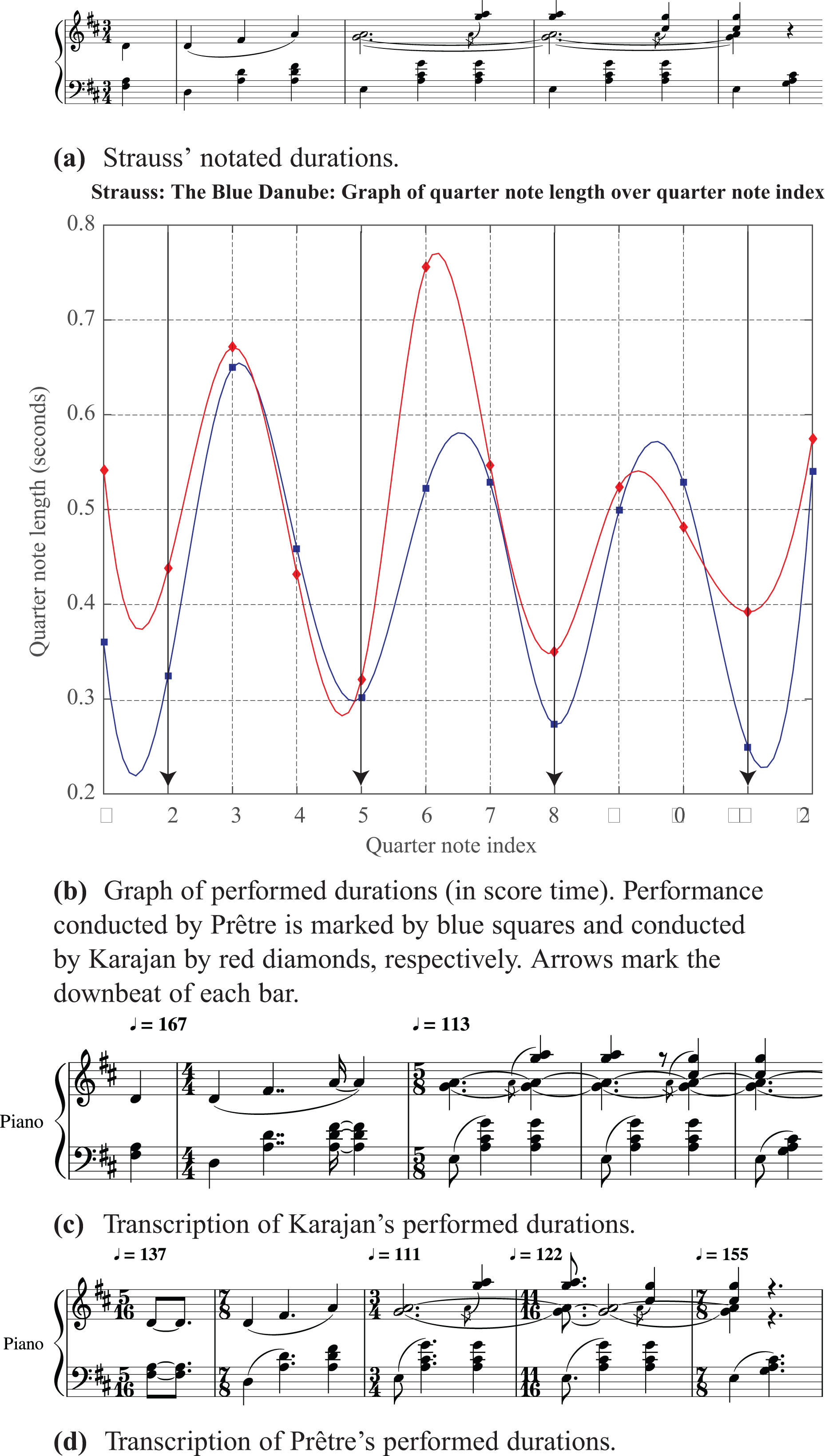
Excerpt from The Blue Danube by Johann Strauss II and analysis and transcription of recorded performances by the Vienna Philharmonic Orchestra conducted by Herbert von Karajan (1987) and Georges Prêtre (2010).

Figure 4(a) shows Strauss’ original notated durations. To extract the performed durations from recorded performances, quarter-note beat onset times (in seconds), ${o_{1}, o_{2}, \dots, o_{N}}$ where N is the total number of onsets, were annotated using Sonic Visualiser (Cannam, Landone, & Sandler, 2010) and checked aurally as well as visually using the audio waveform and spectral information. Beat durations are derived from these onset times, $d_{i} = o_{i + 1} - o_{i}$ , and graphed in Matlab; data interpolation was done using the Matlab spline function. Figure 4(b) shows the resulting graphs generated from performances of The Blue Danube by the Vienna Philharmonic with Herbert von Karajan (1987) and with Georges Prêtre (2010). These particular recordings were chosen because they present two contrasting interpretations of The Blue Danube, which show as divergences in the graphs and the rhythm transcriptions. These differences are all the more interesting because they were created by the same orchestra, albeit 23 years apart, performing under different conductors. In the plot, Figure 4(b), arrows mark the downbeat of each bar. Note that if the music, the score shown in Figure 4(a), was performed literally, exactly as notated, the plot would show only horizontal lines, indicating that all quarter notes have identical durations. This is clearly not the case, as both lines show strong oscillations with varying amplitudes.

The transcription of the performed durations can be described in the form of a heuristic. Suppose the second beat is considered to be early; then the third beat is the one that most closely resembles a full beat duration. Thus, we obtain the baseline beat duration from the third beat, which is assumed to be two or three eighth notes in length. The duration of the third beat served as the reference from which proportional relationships are derived for the preceding beats. Simple ratios—such as 3:2, 2.5:2, 1.5:2, and 2:3—were preferred over more complicated ones. Whether the third beat was two or three eighth notes in length is determined by which interpretation most closely approximated the simpler ratios. Suppose that e_i is the duration of the eighth note when the third beat is i eighth notes long, that is, $e_{i} = d_{b_{3}} / i$ where b_j is the beat index of the j-th beat, $d_{b_{j}}$ is the duration of the b_j-th beat, and $n_{b_{j}}$ is the closest whole number or simple fraction when $d_{b_{j}}$ is divided by e_i. Whether the third beat is two or three eighth notes long is determined by $arg {min}_{i = 2, 3} \sum_{j = 1, 2, 3} ∥ d_{b_{j}} / e_{i} - n_{b_{j}} ∥$ . Note that this technique can be extended to consider other duration categories for the third beat, such as 2.5 eighth notes.

After obtaining the duration ratios, the tempo for any contiguous set of beats, from i to j, is then computed from the total duration, $d = \sum_{k = i}^{j} d_{k}$ , and total quantized score durations, $n = \sum_{k = i}^{j} n_{k}$ , thus the tempo when a beat is two eighth notes long is given by $T = 30 \cdot n / d$ beats/min. The resulting notation is shown in Figures 4(c) and (d). The duration category for the third beat can also be chosen to keep the tempo as unchanging as possible from one bar to the next. For example, the third bar in Figure 4(d) could have been notated with {1.5, 3.5, 2.5} eighth-note durations at basically the same tempo as the preceding bars. However, a metric modulation (change in tempo) gives a simpler notation that keeps the upbeat a quarter note. This simpler notation, which is more friendly to the human eye and requires only a subtle tempo slow-down, is preferred.

Any rhythm transcription necessarily requires some degree of quantization. The original rhythms exists on the real timeline, while the notation is categorical in nature. A transcription thus maps real numbers to duration categories. We are interested in the discrepancy between the real number and the categorical representation. We measure the accuracy of a transcription by the root-mean-square error (RMSE) between the transcribed inter-onset intervals as compared to the inter-onset intervals in the recorded performances. If ${\hat{e}}_{i}$ is the duration of the eighth note given by the tempo at the i th beat, the RMSE is given by

\sqrt{\frac{1}{N} \sum_{i = 1}^{N} {(d_{i} - n_{i} {\hat{e}}_{i})}^{2}}

For the examples shown in Figure 4, the RMSE is 19.1 ms for the Karajan excerpt and 24.9 ms for the Prêtre excerpt, respectively. The numbers are given in Table 1 and graphed in Figure 18 in Appendix A. The small errors show the very slight degree of approximation introduced in the transcription process.

Table 1.

Squared difference between performed and transcribed durations and root-mean-square error (RMSE) (in seconds) for The Blue Danube as performed by the Vienna Philharmonic Orchestra conducted by Herbert von Karajan (1987) and by Georges Prêtre (2010).

Karajan			Prêtre
Perf. dur.	Trans. dur.	Sq. diff.	Perf. dur.	Trans. dur.	Sq. diff.
0.3599	0.3593	0.0000	0.5420	0.5474	0.0000
0.3251	0.3593	0.0012	0.4376	0.4380	0.0000
0.6502	0.6323	0.0003	0.6712	0.6569	0.0002
0.4586	0.4491	0.0001	0.4317	0.4380	0.0000
0.3019	0.2655	0.0013	0.3207	0.2703	0.0025
0.5224	0.5310	0.0001	0.7559	0.8108	0.0030
0.5283	0.5310	0.0000	0.5469	0.5405	0.0000
0.2728	0.2655	0.0001	0.3494	0.3689	0.0004
0.4992	0.5310	0.0010	0.5241	0.4918	0.0010
0.5283	0.5310	0.0000	0.4816	0.4918	0.0001
0.2496	0.2655	0.0003	0.3918	0.3871	0.0000
0.5399	0.5310	0.0001	0.5747	0.5806	0.0000
	RMSE	0.0191		RMSE	0.0249

The difference between the heuristic described here and a more conventional approach, such as transcribing the rhythms by ear, is that the heuristic can be readily translated into a computer program to automate the transcription process. Manual transcription is possible and often desirable for small examples, but scalability is an important consideration for rhythm transcription to be deployable on a large scale for analysis. The method also has the advantage of providing rigorous control over and monitoring of the quantization error.

Many automatic or semi-automatic methods for rhythm transcription exist, see Ycart, Jacquemard, Bresson, and Staworko (2016) and Nakamura, Yoshii, and Sagayama (2017), as well as algorithms for supporting tempo detection (Grosche & Müller, 2011) and tempo change (Quinton, 2017). However, frequency-based methods such as those described by Grosche and Müller (2011) and Quinton (2017) still lack the reactivity required for the frequent meter changes needed to encode free rhythms. The state-of-the-art methods described and evaluated in Nakamura et al. (2017) are designed to recover a score like the one originally written by the composer from the performance. They thus remove the temporal information that is inserted during performance. The work that comes closest to addressing the kind of transcription problem at hand is the interactive rhythm quantification software of Ycart et al. (2016), designed for use by composers as part of Open Music. At present, the software needs further optimization to make it comparable to human efficiency. The method given in this section has the advantage of having been optimized for the special case of the Viennese waltz, which, as it stands, lacks generality. Adaptations tailored to other music styles will be described in the following sections.

In Figure 4, apart from knowing at a glance that the performances are not metronomic, the information embedded in a transcription gives not only the degree of variation, but also the metric modulations, proportional time relations, the precise timing of each note, the distribution of time across the pulses in each bar, and patterns of stress. Figure 4(b) shows Karajan’s more steady (from bar to bar) Viennese waltz rhythm compared with Prêtre’s more variable rhythm, which has the short-long gesture growing larger then shrinking. This observation is reinforced in the notation of Figures 4 (c) and (d). Karajan’s performance could be captured with a constant 5/8 meter after the initial slow start; Prêtre’s performance had to be notated with many more metric modulations—with the beat rate slowing to make the larger gestures that then compress to speed up—and proportional duration category changes. In both cases, the performed durations show marked, and notatable, differences from the original score. The notation thus records the ways in which the score itself is changed and re-shaped by the performer; this is made more obvious by the fact that the original composition and the performed rendition are encoded using the same notational conventions.

Operatic aria

The performer has greatest latitude in creating free-sounding rhythms in solo performance. Among soloists, opera singers are well known for their flexible interpretation of notated rhythms. This second example examines the notation of extreme timing deviations or pulse elasticity in a solo performance of an operatic aria.

Figure 5 shows the duration of each eighth note in an excerpt of “O Mio Babbino Caro” from Giacomo Puccini’s opera, Gianni Schicchi, when performed by Kathleen Battle, Maria Callas, and Kiri te Kanawa. The performed timings of these three recordings have been graphed and analyzed in Chew (2016). The analysis is briefly described here before Callas’ performance is singled out for transcription.

Figure 5.

Eighth-note durations in performances of an excerpt from Puccini’s “O Mio Babbino Caro” by Kathleen Battle, Maria Callas, and Kiri te Kanawa, with tipping points in Callas’ performance highlighted. Data are plotted in score time; vertical gridlines mark the first eighth note of each bar.

As before, the eighth-note beat onsets were annotated and overlaid on the audio signal for inspection in Sonic Visualiser and evaluated aurally for correctness; the eighth-note durations were then obtained from the annotated onsets. This was done for recordings by each of the three sopranos, and the durations plotted on the same graph. To allow for comparisons between the three recorded performances, the three sets of data were plotted in score time, that is, with eighth-note count as the x-axis. Again, interpolation between consecutive duration points was done using the Matlab spline function. The vertical dotted gridlines in the background mark the first eighth note of each bar. The corresponding solo melody is shown beneath the graph itself.

The first thing to note is the large degree of variation in eighth-note durations over the course of even this short excerpt. The baseline eighth-note duration hovers around 0.5 s, indicating that the underlying tempo is approximately 120 eighth notes per minute. In 6/8 time, with three eighth notes to a beat, this translates to a languid pulse of 40 beats per minute. The longest eighth-note duration, corresponding to the highest point in Kiri te Kanawa’s plot, exceeds 5 s, extending almost to 5.5 s. This is a remarkable more than ten-fold increase from the baseline duration. It is such extreme timing deviations that challenge conductors and collaborative artists to virtuosic feats of prediction and adaptation.

While there is a fair degree of commonality in where each performer chooses to invoke the most significant of these excursions from the underlying pulse grid, the ways in which they navigate these and other transitions form unique and often recognizable signatures of the performer or a performance. These time perturbations are the result of practiced choreography to influence the perceived musical context and impose structure on the musical text, to create emphases, and to elicit the desired emotion response from the listener. Such timing variations form the core evidence of the work behind each performance. Thus, it is helpful to be able to see this work represented concretely using an encoding familiar to any musically literate viewer.

In the special case where the stretched pulses coincide with the music structures to elicit a feeling of a roller coaster at the crest of a hill, they are called tipping points, see Chew (2016) or Chew (2017). In Figure 5, cue balls are perched atop each tipping point in Maria Callas’ performance. Not all extreme timing deviations are tipping points, and not all tipping points are signaled by a generous use of time. For an empirical study on what generates tipping points, see Naik and Chew (2017).

Figure 6 focuses on the excerpt within the rectangular box in Figure 5. Figure 6(a) shows the composer’s original notated durations. Figure 6(b) shows Maria Callas’ performed durations in performance (or real) time; listen to this excerpt at https://vimeo.com/127507105. Here, the durations of each eighth note are not plotted against an index of eighth-note counts, but are plotted at the time at which they occur to allow for synchronization with the audio. For a discussion on score time versus performance time, see Chew and Callender (2013). This plot is also interpolated using a spline function.

Figure 6.

Excerpt from “O Mio Babbino” by Giacomo Puccini and Maria Callas’ recorded performance.

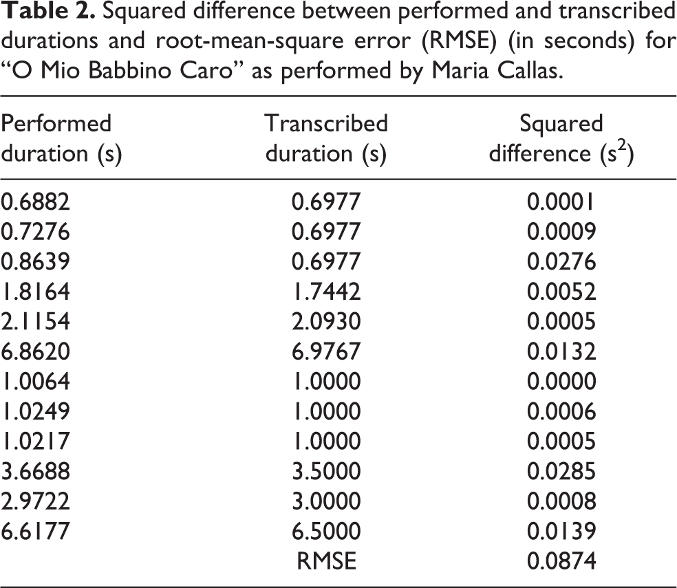
Figure 6(c) shows a transcription of Callas’ recorded performance. The transcription process is straightforward. Because the excerpt begins with a fairly steady (in performance) eighth-note sequence, an underlying pulse grid can be established quickly for the proportional durations. On the repeat of the phrase, the duration of the three-eighth-notes sequence is longer. Hence, the notation was greatly simplified by invoking a metric modulation, from 86 eighth notes per minute to 60 eighth notes per minute, which provided a new unit pulse length rather than persisting with the same unit pulse. The RMSE between the performed and transcribed durations for the notes of the excerpt shown in Figure 6 is 87.4 ms; the precise details are shown in Table 2 and Figure 19 in Appendix A.

Table 2.

Squared difference between performed and transcribed durations and root-mean-square error (RMSE) (in seconds) for “O Mio Babbino Caro” as performed by Maria Callas.

Performed duration (s)	Transcribed duration (s)	Squared difference (s²)
0.6882	0.6977	0.0001
0.7276	0.6977	0.0009
0.8639	0.6977	0.0276
1.8164	1.7442	0.0052
2.1154	2.0930	0.0005
6.8620	6.9767	0.0132
1.0064	1.0000	0.0000
1.0249	1.0000	0.0006
1.0217	1.0000	0.0005
3.6688	3.5000	0.0285
2.9722	3.0000	0.0008
6.6177	6.5000	0.0139
	RMSE	0.0874

From both the graph and the transcription, it is clear that many notes are elongated beyond their notated durations for emphasis and expressive effect. Additional time has been inserted for breaths and to segment the phrases and subphrases. Musically, the first big elongation (the tipping point marked by the leftmost red cue ball in Figure 5) is part of a big ritenuto at the end of the first four bars, the second tipping point stretches the octave leap up to the top A♭, and the third tipping point provides a pause (and breath) before the final ritardando at the last two bars. Unlike conventional ways of marking these expressive gestures, such as by using labels like ritenuto and ritardando, the graph (Figure 6(b)) and notation (Figure 6(c)) show the details of exactly which eighth notes are lengthened, by how much, and which ones not. The notation additionally show the glissandi, marked by distinct note pairs connected by small slurs in the second and fifth bars in Figure 6(b). As indicated by the metric modulation, the two subphrases are performed at different tempi, with the second one a step slower than the first. Visual inspection of Figures 6(c) and 6(a) makes apparent the marked difference between Callas’ performance and the score.

“Happy Birthday”

To show that the literal notation of expressive timing is not confined to classical singing, but also to vernacular forms, we turn our attention to Marilyn Monroe’s (1962) sultry rendition of “Happy Birthday,” performed and recorded live in Madison Square on the occasion of the U.S. President John F. Kennedy’s 45th birthday.

Figure 7(a) shows the conventional notation for “Happy Birthday.” Figure 7(b) shows a graph of the instantaneous tempo at each syllable in Monroe’s rendition of the tune. For greatest precision, the onsets of every syllable were annotated using Sonic Visualiser and checked against the audio signal and spectrogram of the audio signal. Each “Happy” gave the approximate duration of an eighth note and tempo for each new subphrase; sometimes the tempo had to be changed at “to you,” depending on the rate at which the words were sung. The RMSE between the performed and transcribed durations for the notes shown in Figure 7 is 51.5 ms; the details are shown in Table 3 and Figure 20 in Appendix A.

Figure 7.

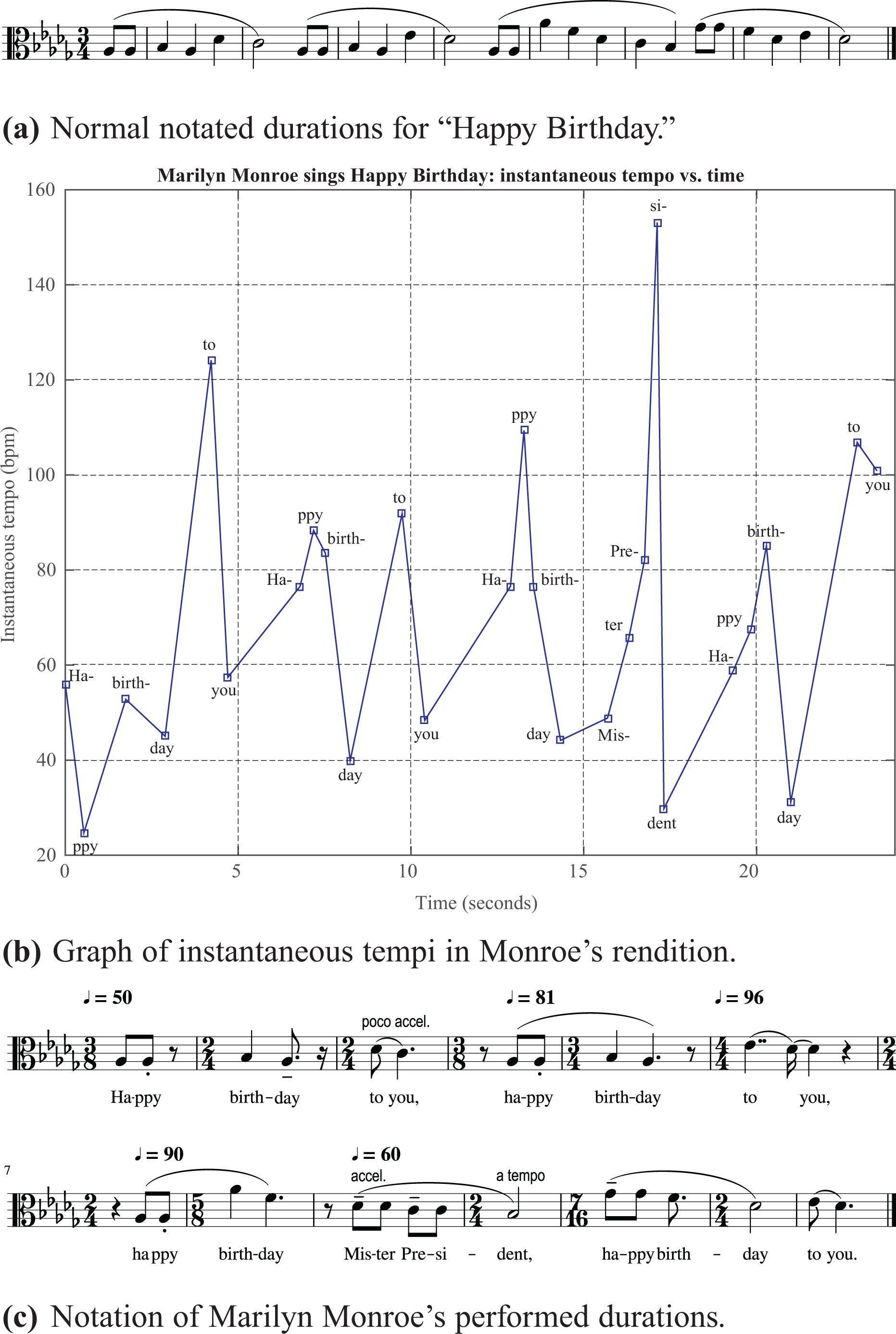
“Happy Birthday” as performed by Marilyn Monroe.

Table 3.

Squared difference between performed and transcribed durations and root-mean-square error (RMSE) (in seconds) for “Happy Birthday” as performed by Marilyn Monroe (1962).

Performed duration (s)	Transcribed duration (s)	Squared difference (s²)
0.5355	0.6000	0.0042
1.2147	1.2000	0.0002
1.1363	1.2000	0.0041
1.3322	1.2000	0.0175
0.4833	0.5172	0.0012
2.0898	2.0690	0.0004
0.3918	0.3704	0.0005
0.3396	0.3704	0.0009
0.7184	0.7407	0.0005
1.5020	1.4815	0.0004
0.6531	0.6250	0.0008
2.4816	2.5000	0.0003
0.3918	0.3333	0.0034
0.2743	0.3333	0.0035
0.7837	0.6667	0.0137
1.3584	1.3333	0.0006
0.6139	0.6000	0.0002
0.4571	0.4545	0.0000
0.3657	0.3659	0.0000
0.1959	0.1961	0.0000
2.0114	2.0000	0.0001
0.5094	0.5000	0.0001
0.4441	0.5000	0.0031
0.7053	0.7500	0.0020
1.9200	2.0000	0.0064
0.5616	0.5000	0.0038
1.1882	1.2500	0.0038
	RMSE	0.0515

Because the syllables map to a variety of duration categories in the score, it is not straightforward to generate a graph of eighth-note durations in a score or real time. Instead, the instantaneous tempo is plotted in real time (as opposed to score time) at the instance of the onset of each syllable. The instantaneous tempo at each syllable, T_s, is computed as a function of the onset times, ${o_{i}}$ (in seconds), and the corresponding syllable’s notated duration, ${s_{i}}$ (in beats), and is given by $T_{s} = 60 \cdot s_{i} / (o_{i + 1} - o_{i})$ . Note that here, local minima signal the pauses or momentary slow-downs, while the peaks mark the fastest-sung syllables. Because Marilyn’s singing of “Happy Birthday” is almost speech-like in its flexible interpretation of time, the transcription led to the simplest notation when invoking multiple metric modulations, practically at every two-word subphrase.

The breathlessness of Marilyn’s singing is marked by the many pauses she takes, which show up as local minima in the plot in Figure 7(b). The many pauses break the usual flow of the melody as well as the phrases in the text. For example, there is a short breath break after almost every instance of the words “Happy birthday.” These breath breaks register as rests in the notation of the performed durations. Portamenti in the sung melody are labeled with slurs in the third, sixth, and last bars. The tempo changes frequently, practically every time the voice re-enters following a breath break. The first “to you” pushes forward (poco accel.), the second “to you” holds back—the glissando arrives at the note before the “you” is vocalized, almost imperceptibly. In the next phrase, the octave leap builds to the climax, which is at a stately 60 beats/min but accelerates to the end of “Mister President” before the final “Happy birthday.”

These three examples demonstrate how performed durations, both carefully sculpted ones and those due to chance, can be captured through transcription using conventional music notation. The following section extends this practice to the transcription of heart rhythms in ECGs of cardiac arrhythmias.

Abnormal heart rhythms

This section considers the transcription of arrhythmic heartbeats using conventional music notation. When the normal electrical activity in the heart is disrupted or altered, arrhythmia results and the heart can beat irregularly, or excessively fast or slow. The ECGs of a heart in sinus (normal) rhythm can make for decidedly uninteresting transcriptions, but the abnormal heart rhythms of arrhythmia are much more varied, offering the potential for producing highly musical rhythm transcriptions.

Take, for example, the trigeminy rhythm, an abnormal heart rhythm in which every third beat is a premature ventricular contraction. Each premature ventricular contraction is followed by a full compensatory pause (a skipped beat) because the heart is still in its refractory period and cannot respond to a stimulus to initiate the next beat. Premature ventricular contractions tend to occur in repeated patterns, aptly named bigeminy (every other beat), trigeminy (every third beat), quadrigeminy (every fourth beat), and so on.

Figure 8 shows a trigeminy rhythm and its transcription. One can imagine extensions to the other premature ventricular contraction rhythms, such as the bigeminy and the quadrigeminy. Note the resemblance of the trigeminy rhythm—regular beat, early beat followed by a compensatory pause, regular beat—to a prototypical Viennese waltz rhythm. The onset of each beat is given by the peak, also known as the R of each QRS complex, in the signal of the upper graph. Given that the standard chart speed is 25 mm/s and a three-beat period is 56 mm on the chart, a beat is $(56 / 25) / 3$ s long and the tempo is given by $60 / ((56 / 25) / 3) \approx 80$ beats/min. This demonstrates how the tempo is computed in the examples to follow. The RMSE between the R–R intervals and the transcribed durations for Figure 8 is 24.8 ms; the details are shown in Table 4 and Figure 21 in Appendix B.

Figure 8.

ECG and transcription of a trigeminy rhythm. (ECG of trigeminal premature ventricular contractions [Online image]. (2013). Retrieved April 16, 2017, from http://floatnurse-mike.blogspot.com/2013/05/ekg-rhythm-strip-quiz-123.html.

Figure 9.

ECG and transcription of atrial fibrillation excerpt Thu 20-07-45 VT 5 beats 210 beats/min (Summary of event) 1 min HR 109 beats/min.

Table 4.

Squared difference between ECG and transcribed durations and root-mean-square error (RMSE) (in seconds) for trigeminy example.

R–R interval (s)	Transcribed duration (s)	Squared difference (s²)
0.7000	0.7500	0.0025
0.5167	0.5000	0.0003
1.0125	1.0000	0.0002
0.7208	0.7500	0.0009
0.4792	0.5000	0.0004
1.0167	1.0000	0.0003
0.7708	0.7500	0.0004
0.5000	0.5000	0.0000
	RMSE	0.0248

The next transcription examples are also derived from surface ECGs; they comprise short summaries from a continuous 18-hour recording taken using a three-lead Holter monitor and show interesting states of atrial fibrillation.

Mixed Meters

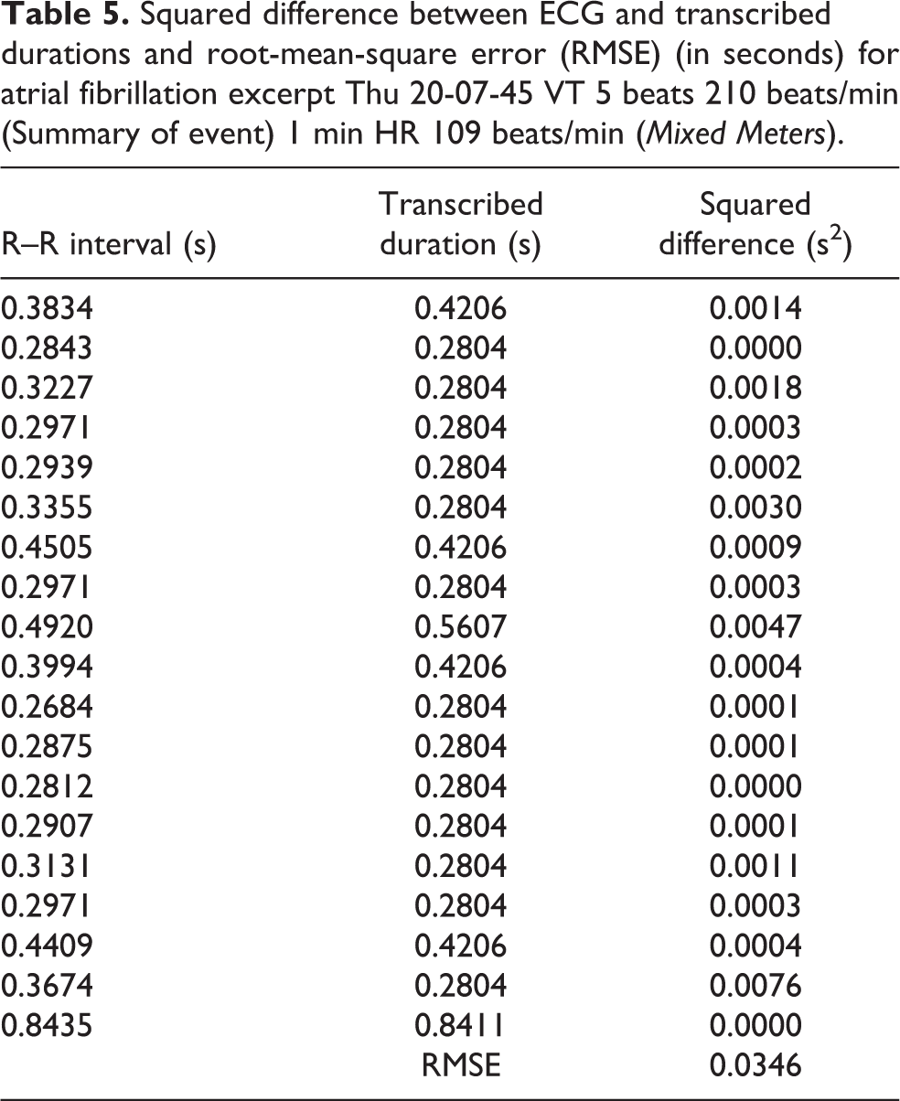
Figure 9 shows the first ECG excerpt and the corresponding transcription of the rhythm. In this example, beats that are slightly more prominent (having greater voltage change) in the ECG are given tenuto-staccato articulation markings; R–R intervals that are slightly short of the full value of a beat duration are marked staccato and R–R intervals that are slightly longer than the full beat value are marked tenuto. The meter changes are assigned to group beats with similar morphology, such as the six wide complex beats in the middle of the sequence, and repeated rhythm patterns, such as the 3 : 2 : 2 pattern. The RMSE between the R–R intervals in the ECG trace and the transcribed durations is 34.6 ms; the details are shown in Table 5 and Figure 22 in Appendix B.

Table 5.

Squared difference between ECG and transcribed durations and root-mean-square error (RMSE) (in seconds) for atrial fibrillation excerpt Thu 20-07-45 VT 5 beats 210 beats/min (Summary of event) 1 min HR 109 beats/min (Mixed Meters).

R–R interval (s)	Transcribed duration (s)	Squared difference (s²)
0.3834	0.4206	0.0014
0.2843	0.2804	0.0000
0.3227	0.2804	0.0018
0.2971	0.2804	0.0003
0.2939	0.2804	0.0002
0.3355	0.2804	0.0030
0.4505	0.4206	0.0009
0.2971	0.2804	0.0003
0.4920	0.5607	0.0047
0.3994	0.4206	0.0004
0.2684	0.2804	0.0001
0.2875	0.2804	0.0001
0.2812	0.2804	0.0000
0.2907	0.2804	0.0001
0.3131	0.2804	0.0011
0.2971	0.2804	0.0003
0.4409	0.4206	0.0004
0.3674	0.2804	0.0076
0.8435	0.8411	0.0000
	RMSE	0.0346

The toggle between 7/8, subdivided as 3 : 2 : 2, and 5/8, subdivided as 3 : 2, meters is reminiscent of the third movement in Libby Larsen’s Penta Metrics (2004). The composer describes the piece as a buoyant dance built around the 7/8 pattern: three beamed eighth notes, eighth note + eighth note rest, eighth note + eighth note rest. Highlighted in the transcription are the patterns of three onsets separated by three-eighth-note and two-eighth-note intervals that are part of the the 3 : 2 : x rhythmic motif. Note that the notation makes these patterns readily discernible.

Figure 10 shows the score of a short composition based (strictly) on the rhythm. It is made up of fragments cannibalized from Penta Metrics, movement III, sometimes transposed so as to fit with the local tonal context. For example, the first bar corresponds to the first bar of Penta Metrics III, the third bar corresponds to the second bar, and the ending chord is identical to that in Larsen’s piece. In between, Bars 2, 4, 5, and 6 are a mix of material, chords and descending octaves, from the sequences in Bars 57 to 60 and Bars 42 to 44, shown in Figures 11(b) and 11(a), respectively.

Figure 10.

Composed fragment based on Thu 20-07-45 VT 5 beats 210 beats/min (Summary of event) 1 min HR 109 beats/min and Libby Larsen’s Penta Metrics, movement III.

Figure 11.

Excerpts from Libby Larsen’s Penta Metrics, movement III.

A video comparing the ECG and rhythm transcription, and the collaged Mixed Meters can be viewed at https://vimeo.com/257248109.

Siciliane

Figure 12 shows the second ECG excerpt and the corresponding transcription of the rhythm. For this example, the most prominent peak in the ECG sequence is highlighted with an accent on the corresponding note, and the wide complex beat with a tenuto mark; other ways to differentiate these waveform details are also possible. The notation in the middle section is simplified by invoking a metric modulation from 94 beats/min to 126 beats/min. This makes the new quarter note 3/4 the value of the previous quarter note, a 25% reduction in time for a beat or a 33% increase in tempo or beat rate. A slight acceleration (marked poco accel.) indicates that the duration of the second beat in the penultimate bar is slightly shorter than the tempo might suggest; the acciaccatura tied to the final note prompts the early onset of the final note, achieving the effect of shortening the penultimate note. The changing meters are chosen to accommodate the different grouping structures. The RMSE between the R–R intervals in the ECG trace and the transcribed durations for Figure 12 is 53.0 ms; the details are given in Table 6 and Figure 23 in Appendix B.

Figure 12.

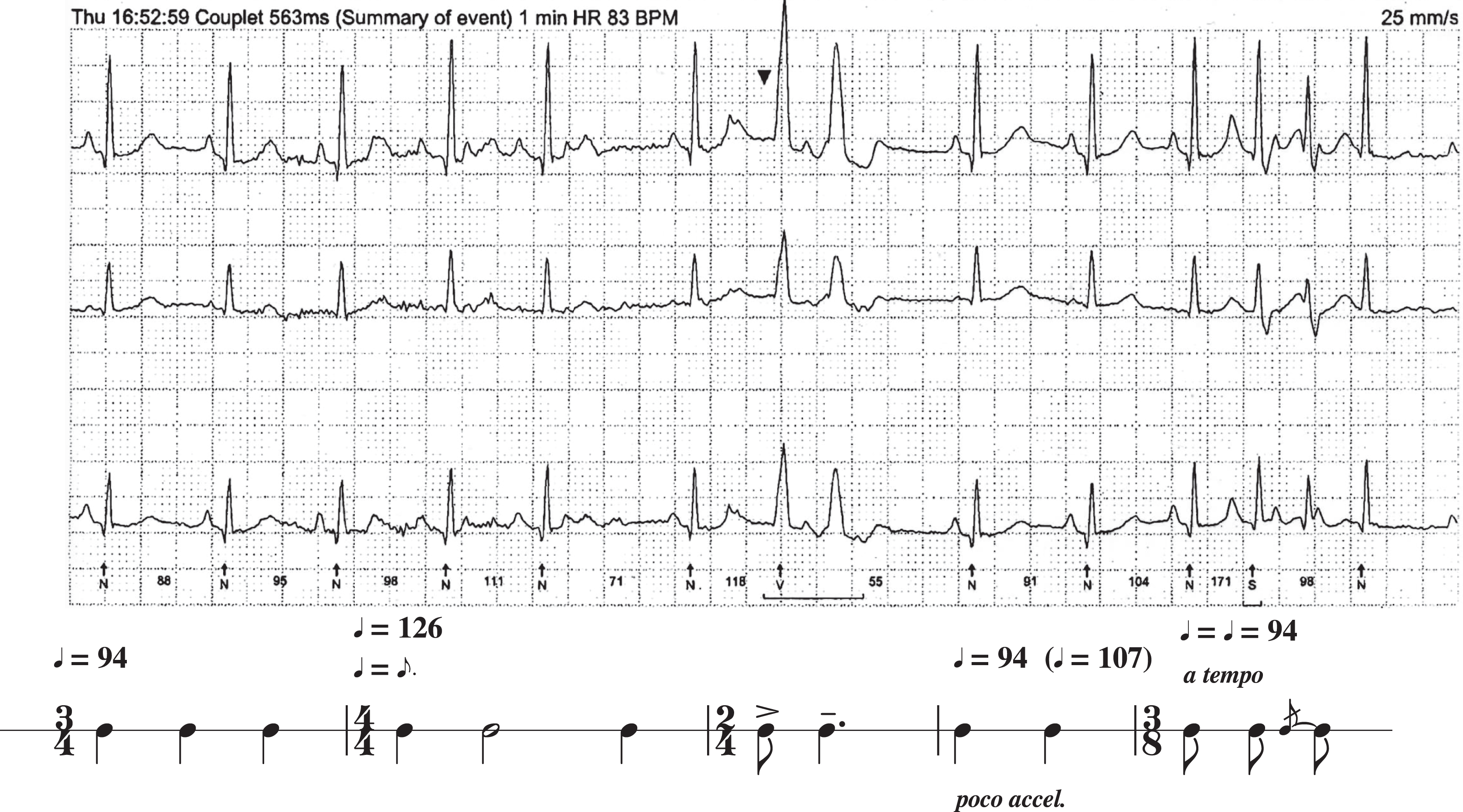
ECG and transcription of atrial fibrillation excerpt Thu 16-52-59 Couplet 563 ms (Summary of event) 1 min HR 83 beats/min.

Table 6.

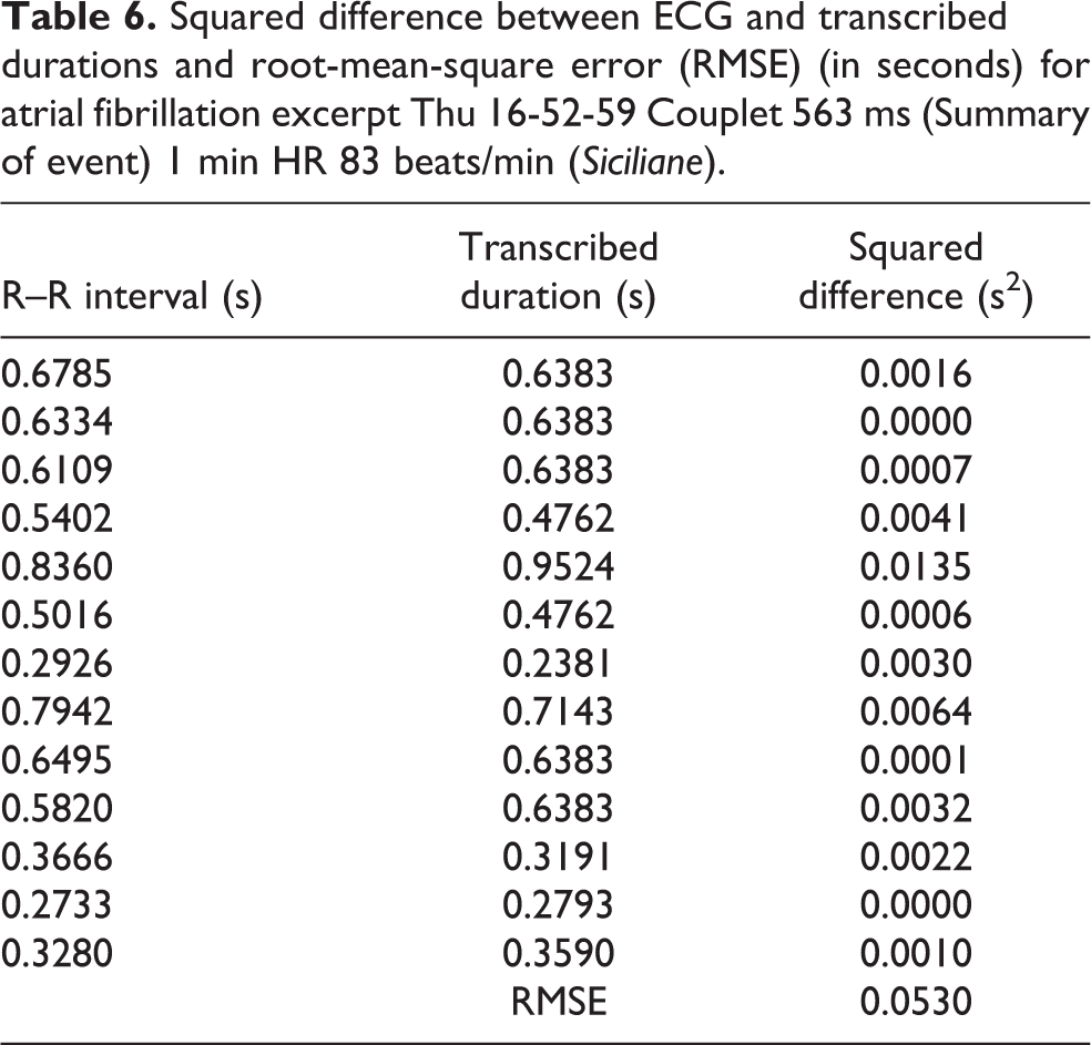
Squared difference between ECG and transcribed durations and root-mean-square error (RMSE) (in seconds) for atrial fibrillation excerpt Thu 16-52-59 Couplet 563 ms (Summary of event) 1 min HR 83 beats/min (Siciliane).

R–R interval (s)	Transcribed duration (s)	Squared difference (s²)
0.6785	0.6383	0.0016
0.6334	0.6383	0.0000
0.6109	0.6383	0.0007
0.5402	0.4762	0.0041
0.8360	0.9524	0.0135
0.5016	0.4762	0.0006
0.2926	0.2381	0.0030
0.7942	0.7143	0.0064
0.6495	0.6383	0.0001
0.5820	0.6383	0.0032
0.3666	0.3191	0.0022
0.2733	0.2793	0.0000
0.3280	0.3590	0.0010
	RMSE	0.0530

This excerpt is slower than the first one, and the long half note in the second bar requires a melodic profile that will fit with this temporal structure. The melody that comes to mind is that of the “Siciliane” in Johann Sebastian Bach’s Flute Sonata No. 2 in E♭ major, BWV 1031, and the piece provides the material for the short composition shown in Figure 13. The original rhythm of the “Siciliane” is lyrical and straightforward, and close to the atrial fibrillation rhythm, but not the same. The melodic profile fits the transcribed rhythm well. Small adjustments are made to the melody so that it fits the rhythm. Figure 14 shows the original melody and the one that has been tweaked to fit the transcribed rhythm. The new melody uses Bars 1, 2, and 4 of the original melody. A passing note was added in the third bar of the modified melody to fit the transcribed rhythm, and two notes from the last bar were inserted to provide a bridge to the concluding bar.

Figure 13.

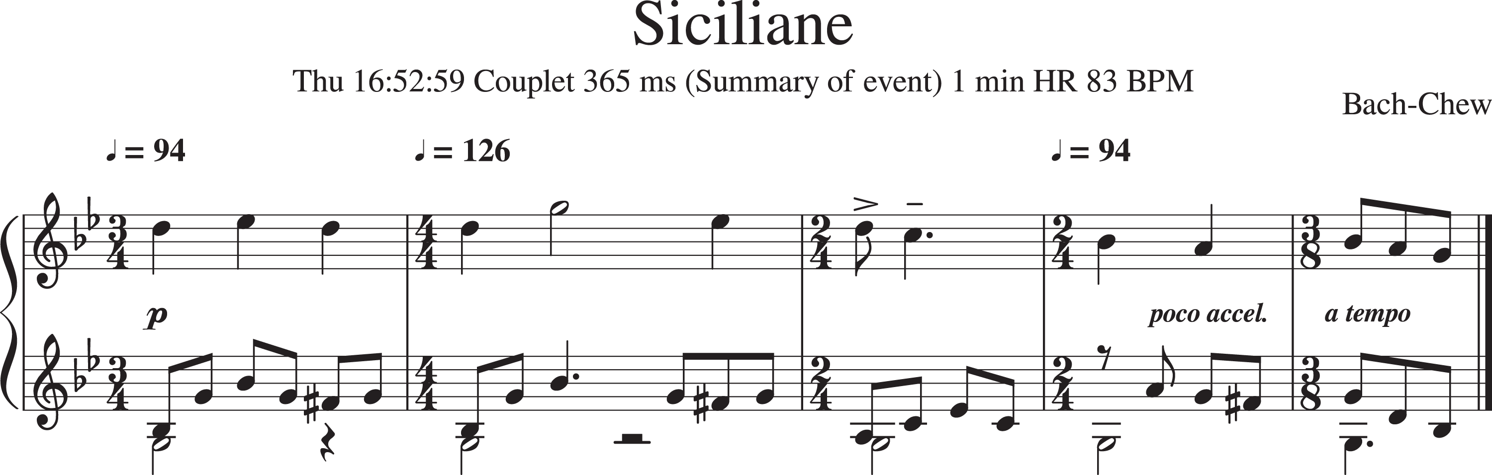
Composed fragment based on transcription of Thu 16-52-59 Couplet 563 ms (Summary of event) 1 min HR 83 beats/min and J. S. Bach’s “Siciliane” from his Flute Sonata No. 2 in E♭ major, BWV 1031.

Figure 14.

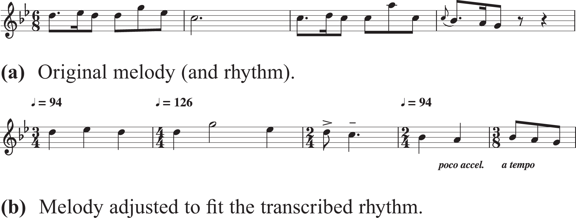
Excerpt from Bach’s “Siciliane” and its modification to fit the transcribed atrial fibrillation rhythm.

An animation showing the correspondence between the ECG and the rhythm transcription, and between the modified Siciliane and the ECG can be viewed at https://vimeo.com/221351463.

Tango

Figure 15 shows the third and final ECG excerpt and the corresponding transcription of its rhythm. As before, the most prominent peaks in the ECG are assigned accent marks; the wide complex beats are given tenuto marks, as are notes of duration slightly longer than their notated values. The RMSE between the R–R intervals in the ECG and the transcribed durations is 40.1 ms; the details are given in Table 7 and Figure 24 in Appendix B.

Figure 15.

ECG and transcription of atrial fibrillation excerpt Thu 17-38-26 VT 4 beats 200 beats/min (Summary of event) 1 min HR 105 beats/min.

Table 7.

Squared difference between R–R intervals in ECG and transcribed durations and root-mean-square error (RMSE) (in seconds) for atrial fibrillation excerpt Thu 17-38-26 VT 4 beats 200 beats/min (Summary of event) 1 min HR 105 beats/min (Tango).

R–R interval (s)	Transcribed duration (s)	Squared difference (s²)
0.3205	0.3191	0.0000
0.4647	0.4800	0.0002
0.4455	0.4800	0.0012
0.3077	0.3191	0.0001
0.4487	0.4800	0.0010
0.5032	0.4800	0.0005
0.3205	0.3191	0.0000
0.3910	0.3191	0.0052
0.4551	0.4800	0.0006
0.3397	0.3191	0.0004
0.2853	0.3191	0.0011
0.2949	0.3191	0.0006
0.2949	0.3191	0.0006
0.3045	0.3191	0.0002
0.4199	0.3191	0.0101
0.5000	0.4800	0.0004
0.3269	0.3191	0.0001
0.3077	0.3191	0.0001
0.5577	0.4800	0.0060
0.4199	0.4800	0.0036
	RMSE	0.0401

Immediately apparent in the transcription are the 3 : 3 : 2 rhythmic pattern, characteristic of the tango, and variations on this pattern, 2 : 3 : x. Capitalizing on the tango reference, the material for the short composition draws from a cadenza-like piano solo in Astor Piazzolla’s Le Grand Tango for cello and piano (1982). The original excerpt from Piazzolla’s piece that provided material for the short composition in Figure 16 is given in Figure 17. In the modified score, the third iteration of the descending sequence is reduced to fit the 7/8 bar by removing the triplet figure. A bridge bar is inserted before material from the first and third bars are combined to reach the concluding bar, which also draws from material in the third bar but with a different finish.

Figure 16.

Composed fragment based on transcription of Thu 17-38-26 VT 4 beats 200 beats/min (Summary of event) 1 min HR 105 beats/min and Astor Piazzolla’s Le Grand Tango.

Figure 17.

Excerpt from Piazzolla’s Le Grand Tango used to fit the atrial fibrillation rhythm.

A video showing the ECG, rhythm transcription, and adapted Tango can be viewed at https://vimeo.com/257253528.

Conclusions and discussions

Having traversed a variety of transcription examples ranging from extreme rhythmic flexibility in performance and the natural flounderings of sight-reading (extreme in a different sense), to the dance-like rhythms of premature ventricular contractions and atrial fibrillation, it is time to reflect on what it means to be able to turn these rhythms accurately to music notation.

A symbolic representation can be used to encode knowledge that can serve as input to machine analysis of these time sequences, thus opening up new approaches for analyzing performed music and arrhythmia sequences. Further work needs to be done to gauge the stability of the transcriptions. Distance metrics can be devised to quantify distances between notations created by different transcribers for the same time sequence to determine consistency. Some key applications of the representation include large-scale deployment of motif detection, similarity assessment, and style classification. For example, after transforming heart period tachograms to elementary rhythm patterns, Bettermann et al. (1999) used a hierarchical pattern scheme to compute the predominance and stability of rhythm pattern classes. Further analyses of the transcribed rhythms could reveal hierarchical structure, like that in Lerdahl and Jackendoff (1996).

The main challenge, for both music performance and cardiac arrhythmia, lies in determining what it is we wish to represent. What are the essential structures of the information streams? What do they mean? Which of these structures are variable and subjective and which are fixed and invariant?

Ideally, transcription should reveal the essential background structure of the temporal experience… In that sense, transcription is a form of analysis in itself. The difficulty of transcribing free rhythm may result from the inadequate nature of the notational system but, at the same time, it signals a deeper analytical problem. Graphic signs can be easily invented once it is clear what we want to represent.

Frigyesi (1993, pp. 60–62)

The changing meters, metric modulations, and detailed note groupings and subgroupings—for example, through the beaming of notes—lead to a number of questions. What can be notated but is not? What is notated and why? Which structures are the result of subjective interpretation and which are fundamental to the temporal sequence? The reality of the metrical groupings implied in each transcription needs to be further tested, for example, by comparing them with expert annotations. More features can be incorporated and larger numbers of transcriptions made to better understand the kinds of patterns that emerge. The transcriptions of abnormal heart rhythms can also serve as new sources of natural-sounding musical rhythms.

The transcriptions of the atrial fibrillation excerpts reveal the vast differences between experiences of irregular heartbeats at different times of the day. Mixed Meters was recorded in the evening at 20:07:45, the Siciliane and the Tango in the late afternoon, at 16:52:59 and 17:39:26, respectively. The rhythms differ not only in rate but also in rhythmic content. Conventional ways of describing atrial fibrillation as simply a condition with irregular heartbeats due to fibrillation in the upper (atrial) chambers of the heart fails to capture the finer features of these time-varying rhythmic structures. It may be that, as for musical styles, information encoded in these rhythmic patterns can be used to distinguish between different forms or phenotypic subtypes of atrial fibrillation, which may be helpful for disease stratification with impact on medical diagnostics and therapeutics.

Footnotes

Acknowledgments

This article is inspired by personal experiences with music performance and cardiac arrhythmias. I am grateful to Dr. Edward Rowland and Professor Pier Lambiase and their respective clinical and catheterization laboratory teams for treating and curing my arrhythmias; Dr. Jem Lane for sharing the story of his Christmas party quiz where he made his colleagues guess arrhythmia types by playing them music of different tempi—this prompted me to create more precise and tangible connections between musical and abnormal cardiac rhythms; and Matron Carolyn Brennan who likens atrial fibrillation to free jazz. Dr. Zongbo Chen helped retrieve my data for the early transcription experiments. Last but not least, Professor Peter Child and Lina Viste Grønli concocted and included me in the Practicing Haydn project, which started me on this marvelous journey.

Declaration of conflicting interests

The author declared no potential conflicts of interest with respect to the research, authorship, and/or publication of this article.

Funding

The author received no financial support for the research, authorship, and/or publication of this article.

Peer review

Ian Pace, City, University of London, Department of Music. Jonathan Berger, Stanford University, Department of Music.

One anonymous reviewer.

Appendix A: Precision of performed music transcriptions

This section contains tables and graphs documenting the difference between the transcriptions and original rhythms derived from the recorded performances and ECGs. The differences are plotted as stem graphs and the tables provide the details of the RMSE calculations. Table 1 provides the numbers for the error calculations for Karajan’s and Prêtre’s recordings of The Blue Danube, with the corresponding stem plots in Figure 18. Table 2 gives the numbers for Maria Callas’ performance of “O Mio Babbino Caro”, with the stem plot in Figure 19; and Table 3 that for Marilyn Monroe’s rendition of “Happy Birthday,” with a stem plot in Figure 20.

Appendix B: Precision of ECG rhythm transcriptions

This section contains tables and graphs documenting the difference between the R–R intervals derived from the ECG traces and the transcribed durations. The squared error between the two are given, as well as the RMSE, in the tables, and stem plots of the difference are given in the figures. Table 4 provides the numbers for the error calculations for the trigeminy example and Figure 21 the corresponding stem plot. Table 5 provides the numbers for the error calculations for the atrial fibrillation excerpt that formed the basis of Mixed Meters, with the corresponding stem plot in Figure 22. Table 6 gives the numbers for the atrial fibrillation excerpt that became Siciliane, with the corresponding stem plot in Figure 23. Table 7 gives the numbers for the atrial fibrillation excerpt for the Tango, with the corresponding stem plot in Figure 24. Not reflected in the numbers and graphs are the effects of the accents and articulation markings incorporated in the transcriptions that mark amplitude (voltage) changes, waveform morphology, or slightly elongated or shortened durations.

References

Ballora

Pennycook

Ivanov

P. C.

Glass

Goldberger

A. L.

(2006). Heart rate sonification: A new approach to medical diagnosis. Leonardo, 37, 41–46.

Bamberger

(2000). Developing musical intuitions: A project-based introduction to making and understanding music complete package. Oxford: Oxford University Press.

Bartlette

Headlam

Bocko

Velikic

(2006). Effects of network latency on interactive musical performance. Music Perception, 24, 49–62.

Bartók

(1942). Photos of Béla Bartók’s transcriptions. Cambridge, MA: Milman Parry Collection of Oral Literature, Harvard College. Retrieved from https://mpc.chs.harvard.edu/gallery/bartok_transcrpt.html

Beaudoin

Kania

(2012). A musical photograph? The Journal of Aesthetics and Art Criticism, 70, 115–127.

Berger

(2016). Vocal materiality and expression in intentionally compromised vocal physiology: The cause and effect of the castrato superstar Luigi Marchesi. Music & Politics, 10. doi: http://dx.doi.org/10.3998/mp.9460447.0010.203

Bettermann

Amponsah

Cysarz

van Leeuwen

(1999). Musical rhythms in heart period dynamics: A cross-cultural and interdisciplinary approach to cardiac rhythms. American Journal of Physiology, 77, H1762–H1770.

Bresson

Assayag

(2011, 11–12). OpenMusic: Visual programming environment for music composition, analysis and research. 19th ACM International Conference on Multimedia (pp. 743–746). New York: ACM.

Callender

(2014). Performing the irrational: Paul Usher’s arrangement of Nancarrow’s Study No. 33, Canon 2:

\sqrt{2}

. Music Theory Online, 20, Retrieved from http://mtosmt.org/issues/mto.14.20.1/mto.14.20.1.callender.html

10.

Cannam

Landone

Sandler

(2010). Sonic Visualiser: An open source application for viewing, analysing, and annotating music audio files. ACM Multimedia 2010 International Conference (pp. 1467–1468). New York: ACM.

11.

Chafe

Cáceres

J.-P.

Gurevich

(2010). Effect of temporal separation on synchronization in rhythmic performance. Perception, 39, 982–992.

12.

Chamberlain

D. S.

(1970). Philosophy of music in the Consolatio of Boethius. Speculum, 45, 80–97.

13.

Cheng

Chew

(2008). Quantitative analysis of phrasing strategies in expressive performance: Computational methods and analysis of performances of unaccompanied Bach for solo violin. Journal of New Music Research, 37, 325–338.

14.

Chew

(2016). Playing with the edge: Tipping points and the role of tonality. Music Perception, 33, 344–366.

15.

Chew

(2017). The mechanics of tipping points: A case of extreme elasticity in expressive timing. In Pareyon

Pina-Romero

Agustín-Aquino

O. A.

Lluis-Puebla

(Eds.), The musical-mathematical mind: Patterns and transformations, pp. 79–88. Cham: Springer.

16.

Chew

Callender

(2013). Conceptual and experiential representations of tempo: Effects on expressive performance comparisons. In: Yust

Wild

Burgoyne

(Eds.), Lecture Notes in Artificial Intelligence: Vol. 7937 (pp. 76–87), Berlin: Springer.

17.

Chew

Child

Grønli

L. V.

(2013). Practicing Haydn: Piano Sonata in E♭ Hob XVI:45, Finale. Retrieved from https://d3mdhum531ctfj.cloudfront.net/exhibitions/Lina_V_Gronli/Practicing_Haydn_Score-1.pdf

18.

Chew

Sawchuk

A. A.

Zimmerman

Stoyanova

Tosheff

Kyriakakis

Volk

(2004). Distributed immersive performance. Proceedings of the 2004 Annual National Association of the Schools of Music (pp. 85–94). Reston: National Association of Schools of Music.

19.

Clayton

M. R. L.

(1996). Free rhythm: Ethnomusicology and the study of music without metre. Bulletin of the School of Oriental and African Studies, University of London, 59, 323–332.

20.

Coltrane

(1999). John Coltrane improvised saxophone solos. (Transcribed by Sickler

). Los Angeles: Alfred Publishing Co.

21.

Cook

(1987). Structure and performance timing in Bach’s C major Prelude (WTCI): An empirical study. Music Analysis, 6, 257–272.

22.

Cook

(2013). Beyond the score: Music as performance. Oxford: Oxford University Press.

23.

Davids

(1995). Heartsongs: Musical mappings of the heartbeat. Wellesley, MA: Ivory Moon Recordings.

24.

Ellington

(1971). Concerto for Cootie: From the study scores series: the Ellington orchestra. (Transcribed by Berger

& Campbell

). Los Angeles: United Artists Music.

25.

Evans

(1967). Bill Evans plays. New York: Ludlow Music.

26.

Farbood

(2004). Hyperscore: a graphical sketchpad for novice composers. IEEE Computer Graphics and Applications, 24, 50–54.

27.

Field

(2010). Music of the Heart. The Lancet, 376, 2074.

28.

Frigyesi

(1985). Between rubato and rigid rhythm: A particular type of rhythmical asymmetry as reflected in Bartók’s writings on folk music. Studia Musicologica Academiae Scientiarum Hungaricae, 24, 327–337.

29.

Frigyesi

(1993). Preliminary thoughts toward the study of music without clear beat: The example of “flowing rhythm” in Jewish “Nusah.” Asian Music, 24, 59–88.

30.

Grønli

L. V.

Child

Chew

(2013). Practicing Haydn. Kunsthall Stavanger, 10 November 2013. Retrieved from https://kunsthallstavanger.no/en/exhibitions/practicing-haydn

31.

Grosche

Müller

(2011). Tempogram toolbox: MATLAB implementations for tempo and pulse analysis of music recordings. International Conference on Music Information Retrieval. Victoria: International Society for Music Information Retrieval.

32.

Herremans

Chew

(2017). MorpheuS: Generating structured music with constrained patterns and tension. IEEE Transactions on Affective Computing. doi: 10.1109/TAFFC.2017.2737984

33.

Hold

(1970). The notation of bird-song: A review and a recommendation. International Journal of Avian Science, 112, 151–172.

34.

Hope

Vickery

(2015). The Decibel Scoreplayer—A digital tool for reading graphic notation. In International Conference on Technologies for Music Notation and Representation. Paris, France: Institut de Recherche en Musicologie (IReMus).

35.

Houle

(2000). Meter in music, 1600–1800: Performance, perception, and notation. Bloomington: Indiana University Press.

36.

Jarrett

(1991). Keith Jarrett: The Köln Concert: Original transcription, piano. (Transcribed by Kishinami

& Yamashita

), ED7700. Mainz: B. Schott Söhne.

37.

Knyt

E. E.

(2010). Ferruccio Busoni and the ontology of the musical work: Permutations and possibilities. (PhD dissertation). Stanford University, Stanford.

38.

Kosta

Bandtlow

Chew

(2014). Practical implications of dynamic markings in the score: Is piano always piano? 53rd Audio Engineering Society International Conference on Semantic Audio. New York: Audio Engineering Society.

39.

Laennec

R. T. H.

(1826). Traité de l’auscultation médiate et des maladies des poumons et du coeur. Nouvelle Édition, Brussels: La Librairie Médicale et Scientifique.

40.

Lerdahl

Jackendoff

R. S.

(1996). A generative theory of tonal music. Cambridge: MIT Press.

41.

Marchesi

(1792). Air de Zingarelli, Ms. BC 11550. (Transcription by Pichl

). Brussels: Bibliothque des Conservatoires royaux de Bruxelles.

42.

Marsh

(1994). Heroic motives: Roger Marsh considers the relation between sign and sound in ‘complex’ music. The Musical Times, 135, 83–86.

43.

McKee

(2011). Decorum of the minuet, delirium of the waltz: A study of dance-music relations in 3/4 time. Bloomington: Indiana University Press.

44.

Meireles

A. R.

Simões

A. R. M.

Ribeiro

A. C.

de Medeiros

B. R.

(2017). Musical speech: A new methodology for transcribing speech prosody. Interspeech (pp. 334–338). Stockholm, Sweden: International Speech Communication Association.

45.

Messiaen

(1956). Oiseaux Exotique for piano and small orchestra. Vienna: Universal Edition.

46.

Monroe

(1962). “Happy Birthday”, 19 May 1962, Madison Square Garden, New York, U.S. Retrieved from https://youtu.be/EqolSvoWNck

47.

Moody

G. B.

(2013). LightWAVE: Waveform and annotation viewing and editing in a Web browser. Computing in Cardiology Conference. (pp. 17–20). Piscataway: IEEE.

48.

Morton

(1986). Ferdinand “Jelly Roll” Morton: The collected piano music. (Transcribed by Dapogny

). New York: G. Schirmer.

49.

Naik

Chew

(2017). Tipping points, pulse elasticity and tonal tension: An empirical study on what generates tipping points. International Conference on Music Information Retrieval. Victoria: International Society for Music Information Retrieval. Retrieved from https://ismir2017.smcnus.org/lbds/Naik2017.pdf

50.

Nakamura

Yoshii

Sagayama

(2017). Rhythm transcription of polyphonic piano music based on merged-output HMM for multiple voices PDF external site demo. IEEE/ACM Transactions on Audio, Speech and Language Processing, 25, 794–806.

51.

Ohriner

(2016). Metric ambiguity and flow in rap music: A corpus-assisted study of Outkast’s Mainstream (1996). Empirical Musicology Review, 11, 153–179.

52.

Orzessek

Falkner

(2006). Sonification of autonomic rhythms in the frequency spectrum of heart rate variability. 12th International Conference on Auditory Display. London, UK.

53.

Parker

(1978). Charlie Parker Omnibook. (Transcribed by Aebersold

& Stone

). New York: Atlantic Music Corporation.

54.

Philip

(1992). Early recordings and musical style: Changing tastes in instrumental performance, 1900–1950. Cambridge: Cambridge University Press.

55.

Prêtre

(2010). The Blue Danube, Vienna Philharmonic New Year’s Concert, Vienna, Austria. Retrieved from https://youtu.be/NlFBWo-Cbz8

56.

Qiu

Hong

(2016). A novel method for mining semantics from patterns over ECG data. Workshops of the Thirtieth AAAI Conference on Artificial Intelligence: Expanding the Boundaries of Health Informatics Using AI. Palo Alto: Association for the Advancement of Artificial Intelligence.

57.

Quinton

(2017). Towards the automatic analysis of metric modulation (PhD dissertation), Queen Mary University of London, London.

58.

Repp

(1992). Analysis of timing in music performance. Journal of the Acoustic Society of America, 92, 2546–2568.

59.

Sborgi Lawson

F. R.

(2012). Consilience revisited: Musical and scientific approaches to Chinese performance. Ethnomusicology, 56, 86–111.

60.

Segall

H. N.

(1962). Evolution of graphic symbols for cardiovascular sounds and murmurs. British Heart Journal, 24, 1–10.

61.

Silva

Moody

G. B.

(2014). An open-source toolbox for analysing and processing PhysioNet databases in MATLAB and Octave. Journal of Open Research Software, 2, e27. Retrieved from https://physionet.org/physiotools/wfdb.shtm

62.

Simões

A. R. M.

Meireles

A. R.

(2016). Speech prosody in musical notation: Spanish, Portuguese and English. Speech Prosody. Baixas: International Speech Communication Association.

63.

Siraisi

N. G.

(1975). The music of pulse in the writings of Italian academic physicians (fourteenth and fifteenth centuries). Speculum, 50(4), 689–710.

64.

Spiro

Gold

Rink

(2016). Musical motives in performance: A study of absolute timing patterns. In Smith

J. B. L.

Chew

Assayag

(Eds.): Mathematical conversations: Mathematics and computation in performance composition (pp. 109–128). Singapore: World Scientific.

65.

Steele

(1775). An essay towards establishing the melody and measure of speech. Menston: Scholar Press Ltd.

66.

Syed

Stultz

Kellis

Indyk

Guttag

(2010). Motif discovery in physiological datasets: A methodology for inferring predictive elements. ACM Transactions on Knowledge Discovery Data, 4, 2.

67.

Todd

N. P. M.

(1992). The dynamics of dynamics: A model of musical expression. Journal of the Acoustical Society of America, 91, 3540–3550.

68.

Tucker

(1982). Behind the beat with Mark Tucker. American Music Review, 12, 11.

69.

von Karajan

(1987). The Blue Danube, Vienna Philharmonic New Year’s Concert, Vienna, Austria. Retrieved from https://youtu.be/I-X3C1w77Eg

70.

Votava

Berger

(2011). The Heart Chamber Orchestra: An audio-visual real-time performance for chamber orchestra based on heartbeats. eContact!—Online Journal of the Canadian Electroacoustic Community, 14. Retrieved from http://econtact.ca/14_2/votava-berger_hco.html

71.

Yang

Chew

Rajab

(2013). Vibrato performance style: A case study comparing erhu and violin. 10th International Symposium on Computer Music Multidisciplinary Research (pp. 904–919). Marseille, France: Laboratoire de Mécanique et d'Acoustique.

72.

Ycart

Jacquemard

Bresson

Staworko

(2016). A supervised approach for rhythm transcription based on tree series enumeration. International Computer Music Conference. San Francisco: International Computer Music Association.

73.

Yokohama

(2002). Heart rate indication using musical data. IEEE Transactions on Biomedical Engineering, 49, 729–733.

Notating disfluencies and temporal deviations in music and arrhythmia

Abstract

Keywords

Introduction

Transcription

Representing performed music

Musica humana

Transcription process

Rhythmic disfluencies

Choreographed rhythms

Viennese waltz

Operatic aria

“Happy Birthday”

Abnormal heart rhythms

Mixed Meters

Siciliane

Tango

Conclusions and discussions

Footnotes

Acknowledgments

Declaration of conflicting interests

Funding

Peer review

Appendix A: Precision of performed music transcriptions

Appendix B: Precision of ECG rhythm transcriptions

References