Sage Journals: Discover world-class research

Abstract

Segmenting continuous sensory input into coherent segments and subsegments is an important part of perception. Music is no exception. By shaping the acoustic properties of music during performance, musicians can strongly influence the perceived segmentation. Two main techniques musicians employ are the modulation of tempo and dynamics. Such variations carry important information for segmentation and lend themselves well to numerical analysis methods. In this article, based on tempo or loudness modulations alone, we propose a novel end-to-end Bayesian framework using dynamic programming to retrieve a musician's expressed segmentation. The method computes the credence of all possible segmentations of the recorded performance. The output is summarized in two forms: as a beat-by-beat profile revealing the posterior credence of plausible boundaries, and as expanded credence segment maps, a novel representation that converts readily to a segmentation lattice but retains information about the posterior uncertainty on the exact position of segments’ endpoints. To compare any two segmentation profiles, we introduce a method based on unbalanced optimal transport. Experimental results on the MazurkaBL dataset show that despite the drastic dimension reduction from the input data, the segmentation recovery is sufficient for deriving musical insights from comparative examination of recorded performances. This Bayesian segmentation method thus offers an alternative to binary boundary detection and finds multiple hypotheses fitting information from recorded music performances.

Keywords

Bayesian inference probabilistic segmentation music expressivity music performance musical prosody

Introduction

Music is increasingly viewed as performance (Cook, 2014), in contrast to the long-held view of music as artifact, as writing, as score. However, studying the ephemeral medium of music as it unfolds in time poses significant challenges. Extracting meaningful musical structures from musical performance lacks the constants afforded by the notated score. Finding musical structures relevant to the act and perception of performance adds complexity to the undertaking. While tools exist to extract features and basic musical structures from recorded performances, turning these extracted parameters into pertinent representations of the music remains an important computational challenge. Here, we propose a way to abstract, in a nuanced way, the performer's projected structural understanding of the music s/he is playing, and to compare any two such structural representations.

When performing a piece, musicians not only have in mind the notes they are about to play, but also some intuitions as to how the musical material such as notes group together into coherent ideas (Gody et al., 2010), how they relate one to another (Lewin, 2007), and which ideas could be made more prominent and others sublimated (Cadwallader, 1998) during performance (Mazzola, 2011). Some of these intuitions may derive from experience, some may be formulated in real-time amid performance, parts of it may coalesce into some mental conceptions of the music. All these notions serve to guide the performer's expressive choices (Rink, 1995), which in turn influence how the listener hears the music (Clarke, 2005). Using the tools at their disposal, within the constraints of the physical properties of their instrument, the performance conventions they wish to adopt (or reject), their own bodily form and technical abilities, performers manipulate timing, articulation, and dynamics to shape the music (Leech-Wilkinson, 2017) to convey segmentation, prominence, and affect (Palmer & Hutchins, 2006) to the listener. These functional acoustic variations are referred to as musical prosody.

The varying of tempo (beat rate) and loudness (perceived sound pressure) form a main focus of performance research (Chew, 2023; Langner & Goebl, 2003; Kosta et al., 2016, 2018a). A well-documented practice is the arching of tempo and/or dynamics to mark phrases. Performers tend to convey phrases through accelerando–deccelerando and crescendo–decrescendo patterns (Todd, 1992; Gabrielsson, 1987), which also serve as cues for how the performer or listener segments the musical material.

The phrases that performers highlight in this way are approximately nonoverlapping and cover the whole piece; hence, defining a segmentation. In this article, we focus on the problem of recovering such a segmentation from the prosody in a recorded music performance. The question we ask is: Given a recorded performance, can we reverse engineer it to uncover the performer's segmentation of the piece from the musical prosody alone, without the notes?

Segmentation is an important part of perception (Zacks & Swallow, 2007), and it is no surprise that it is widely studied in multimedia research, including for images (Haralick & Shapiro, 1985), video (Koprinska & Carrato, 2001), and audio (Sakran et al., 2017). In particular, music segmentation has received a lot of attention (Paulus et al., 2010; Nieto et al., 2020), with most automatic approaches partitioning the music according to criteria of repetition (Guichaoua, 2017; Lascabettes et al., 2022b) and novelty (Lascabettes et al., 2022a). Relatively few methods have focused on musical prosody as a source of algorithmic segmentation cues. Widmer and Tobudic (Widmer & Tobudic, 2003) fit quadratic models to performance features (instantaneous tempo and loudness)¹ given a known multilevel segmentation; while their aim was not to segment the music, this work highlighted the correspondence between phrase arcs and segmentation boundaries. Chuan and Chew (2007) turned the approach around by introducing joint estimation of segmentation boundaries and parameters for an arc model, which yields a segmentation solution rather than requiring one. This was later refined by Stowell and Chew (2013) who added a Bayesian prior to steer the estimation toward more plausible solutions. Like Chuan and Chew (2007) and Stowell and Chew (2013), we choose to focus exclusively on loudness and instantaneous tempo data, discarding all direct score information. This represents a deeper conceptual shift than what might be immediately obvious. By focusing on musical prosody alone, what is being segmented is no longer the piece as written in the score, but the acoustic performance as realized by the musician. Although, as we can observe in our results, the score structure can be partially carried over through the performance, the extracted structure is of a different nature, barring direct comparisons with repetition- and novelty-based methods. Another characteristic which sets this work apart from most of the existing literature, including that on performance segmentation is that, unlike previous methodologies, we use an end-to-end Bayesian approach, aiming for a credence-based, multiple solution output rather than a single solution.

Indeed, research shows that listeners, when asked to judge the segmentation of a recorded piece of music, sometimes disagree about the exact placement of the boundaries and their existence or relevance (Smith et al., 2014; Wang et al., 2017; Nieto et al., 2020). This indicates that the segmentations that performers project may not be perceived universally the same way. Since part of the disagreement can be traced to listeners focusing on different aspects of the music (Smith et al., 2014; Smith & Chew, 2017) such as rhythm, melody, harmony, or timbre, it seems illusory to expect to recover a sole best projected segmentation based on only one or two features. This calls for a representation of segmentation results that allows for multiple plausible solutions. In short, prior work on music segmentation typically attempts to output a final best guess of the segmentation; even those adopting a Bayesian approach ultimately only output a best answer. In contrast, we aim to provide a more nuanced representation of the segmentation solution in which multiple segmentation hypotheses can co-exist. Such an approach has proven useful in cases where insufficient data is available, as in Rupprecht et al. (2017) for computer vision. These segmentation hypotheses can then be refined, either based on a manual complementary analysis or by using additional sources of data.

To achieve this goal of returning multiple solutions, we adopt a Bayesian framework. Bayesian approaches have been applied to problems in music such as beat tracking (Degara et al., 2011), and key finding and meter induction (Temperley, 2007). In our Bayesian context, we examine all possible segmentations and let those that are supported by the performance features rise to the fore. The total number of segmentations is exponential according to the number of possible segmentation points, which makes a naïve approach both unusable and computationally intractable. By focusing on the credence of individual boundaries or individual segments, we are able to use a new dynamic programming algorithm to compute these probabilities efficiently.

Focusing on the credence of individual segments, we propose a new representation of the multiple segmentation hypotheses, which we call the expanded segment credence map. This map provides an overview of the flow of segments one into another, analogous to a segmentation lattice, a directed graph where each node represents a plausible segment and is connected to the other plausible segments that start when it ends. In contrast to the lattice where each node is a discrete segment, we do not discard nuance about the endpoints of segments, such as whether there remains uncertainty about the existence or exact location of any given boundary.

We also introduce a method based on unbalanced optimal transport to compare two segmentations resulting from two performances. The use of unbalanced optimal transport provides a temporal tolerance between boundaries and flexibility in the number of boundaries between two segmentations derived from performances. Therefore, this distance provides a method of measuring similarity between two musical performances, taking only the segmentation induced in the performance into account. In addition to measuring similarity, this distance highlights where estimates agree or disagree. This allows us to understand similarities between the ways different performers conceptualize the music to produce the recorded performances.

To test the algorithm and demonstrate its use on real data, we use selected recordings from the MazurkaBL dataset (Kosta et al., 2018b), which contains about 2000 performances across Chopin's 49 mazurkas and the corresponding loudness and instantaneous tempo data. As Romantic-era solo piano pieces, almost all of the performer's expressiveness lies in the dynamics, pedal, and timing (including rubato) modulations, which are each sequentially quantifiable.

The remainder of the article is organized as follows: the first section presents the Bayesian model we use to assign credence to segmentations, as well as the recursive formulae which lets us compute these credences efficiently; the next section shows how this information can be processed to be accessible to humans and shares a few insights that arise from direct examination of the outputs; our penultimate section proposes the use of unbalanced optimal transport to reveal similarities and differences between segmentations from different interpretations of the same piece; finally, we provide some concluding remarks and point to applications and leads for future developments of this method.

Modeling and Boundary Credence Estimation

We have assumed that a performance is driven (in part) by the performer's segmentation of the piece. However, this segmentation is not directly accessible, as it resides in the performer's mind: it can only be inferred from the data that it has influenced, in particular the tempo and loudness of the performed music, which are readily quantifiable. Thus, we use Bayesian inference to update, using observed data, a model of the plausible segmentations. For the Bayesian inference, we also need a model of how segmentation is going to drive the data. This model we use comprises of two parts: an overall theory of the behavior of segments, and a model of how segmentation decisions affect the prosody.

First, we need an overall model (a theory) of which segmentations are likely before observing any data. This is similar in a broad sense to the method employed in Sargent et al. (2017). For example, using their overall model, a segmentation that would divide a piece into a few very short segments and a very long one seems unlikely to be correct, whereas a segmentation comprising segments of similar and phrase-length sizes could be much more plausible, before even considering the data.

Second, a specific model describing how a given segmentation affects the performance data is also required. Loudness and/or tempo have been shown to exhibit arch shapes delineating phrases (Todd, 1992; Gabrielsson, 1987), particularly in romantic era music. Examples of phrase marking tempo arcs in Artur Schnabel's recording of Beethoven's “Moonlight” Sonata, with accelerations at the beginnings of phrases and deccelerations near the end, can been seen in Figure 1. Empirically, while the edges of some phrases may be clear, others are less obvious. As a compromise between model complexity and modeling error,² a piecewise concave quadratic model has been chosen as the specific model. This specific model drives the data and the kinds of arcs that we are likely to see.

Figure 1.

(a) Instantaneous tempo in Artur Schnabels performance of Beethoven’s “Moonlight” Sonata with corresponding score (m. 115); and (b) with three levels of tempo arcs at the initial four bars outlined on the plot. Reproduced from Chew (2016a) (Figure 5, p. 133, and Figure 6, p. 135).

In this article, we shall assume that arcs are independent one from another, that is, that modulations in one arc do not affect those in others, and that the plausibility of an arc depends only on its beginning and end. This assumption is somewhat unrealistic, as a performer may be more likely to shape a repeated section in the same way (or conversely in a contrasting fashion) across all its occurrences, but it is necessary for our use of dynamic programming to break down the computations in a tractable way. An added benefit of this independence assumption is that it ensures that the overall and specific models are decoupled, meaning that either model can easily be replaced by an alternate model without major repercussions.

This two-tiered model mirrors the one used in Stowell and Chew (2013), with minor changes to the priors. The main difference is the goal of the computations. In the current method, our objective is to look for the posterior credence of all segmentations, summarized through credence values on the arcs or boundaries, rather than to seek the segmentation of maximal credence.

In the following subsections, we first describe the input and output of the method and the underlying assumptions; we then show how this output can be efficiently computed from the segmentation prior and the segment-wise data likelihood; we conclude by describing the arc model we use to compute these likelihoods.

Problem Statement and Notations

We view the prosodic feature extracted from the recorded performance as a sequence of N instantaneous tempo or loudness values $D$ , each corresponding to the value at a beat. We denote $D [i, j]$ as the sequence slice from indices i to and including j ( $0$ -indexed).

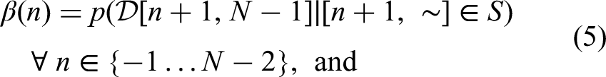
We consider that the performance segmentation consists of a succession of nonoverlapping, consecutive intervals that can only change on the beat. Notation-wise, we represent this as a set S of integer intervals; if $[i, j] \in S$ , there is an arc starting at data index i and ending at j, and the next arc (if there is one) would start at data index $j + 1$ . We introduce shorthands $[i, \sim] \in S$ and $[\sim, j] \in S$ to signify that an arc starts at index i (respectively ends at $j$ ), regardless of its other end (that is to say, $[i, \sim] \in S g t \Leftrightarrow g t \exists k : [i, k] \in S$ ).³

Our aim is to infer information about the posterior credence of S, mainly by marginalizing against boundaries to obtain posterior boundary credences $p ([\sim, j] \in S ∣ D)$ or against arcs to obtain posterior arc credences $p ([i, j] \in S ∣ D)$ . We refer to the sets of these values as the boundary credence profile and the arc credence matrix of a piece, respectively, although the matrix will be further transformed for the sake of visualization.

The assumption of independence across arcs is formalized in two ways, one for the data and one for the prior:

\begin{aligned} \forall n, D [0, n] ⊥ ⊥ D [n + 1, N - 1] ∣ [\sim, n] \in S \\ \forall k, l, i, j s . t . k < l < i < j, \end{aligned}

(1)

p ([i, j] \in S ∣ [i, \sim] \in S, [k, l] \in S) = λ (i, j)

(2)

where

λ (i, j) = p ([i, j] \in S ∣ [i, \sim] \in S)

. In less formal terms, this means that the data before a boundary has no effect on the data after that boundary, and that the prior on the end of a segment does not depend on previous segments.

Finally, we assume that the first and last beats are respectively the first and the last beats of the first and last arcs, that is, $[0, \sim] \in S$ and $[\sim, N - 1] \in S$ . The $λ$ function is then sufficient to define the entire prior on the segmentations⁴ and operates as a parameter for the method. We use functions that are translation invariant, meaning they act as a prior on the length of any segment, but this is not a requirement.

Adapted Forward–Backward Algorithm

Here we show how the posterior marginals can be computed efficiently by using a similar process to that of the forward–backward algorithm, which bears resemblance to some Bayesian changepoint detection algorithms (Rigaill et al., 2012; Fearnhead & Liu, 2011).

By applying Bayes’ formula, we have the following:

p ([\sim, n] \in S ∣ D) = \frac{p (D ∣ [\sim, n] \in S) p ([\sim, n] \in S)}{p (D)} .

(3)

None of these terms are trivial to compute. However, using the assumption that data across arcs are independent, we can rewrite Equation 3 using the so-called forward and backward quantities

α (n)

and

β (n)

, defined as⁵

α (n) = p (D [0, n], [\sim, n] \in S) \forall n \in {0 \dots N - 1},

(4)

β (n) = p (D [n + 1, N - 1] ∣ [n + 1, \sim] \in S) \forall n \in {- 1 \dots N - 2}, and

(5)

p ([\sim, n] \in S ∣ D) = \frac{α (n) β (n)}{α (N - 1)} \forall n \in {0 \dots N - 1} .

(6)

where

α

= joint probability between the prior credence of a boundary and the joint probability of the data up to that boundary; and

β

= probability of observing the data from a boundary to the end, conditioned on that boundary being present. Broadly speaking,

α

and

β

split the probability of observing the overall data according to a hypothetical boundary at n, and combine to give the credence value p. Boundaries are not truly random variables. The Bayesian approach treats such unknowns as distributions. Since we are not predicting random processes, which have associated probabilities, the computations work with credences, which express a belief. For example, p can be a posterior credence (as in Equation 6) or a prior credence (as in Equation 3).

Recursive formulae can be derived (see supplementary material) for these new quantities, using $κ (i, j) = p (D [i, j] ∣ [i, j] \in S)$ as represented by

α (n) = \sum_{i = 0}^{n - 1} α (i - 1) \times λ (i, n) \times κ (i, n), and

(7)

β (n) = \sum_{i = n + 2}^{N - 1} β (i) \times λ (n + 1, i) \times κ (n + 1, i),

(8)

showing that both quantities can be computed respectively forward and backward by summing, over possible arcs, their previously computed values, weighted by the prior on that arc and the likelihood of the corresponding data slice. This can be done efficiently using dynamic programming, especially if the prior is null for arcs over a maximum length.⁶

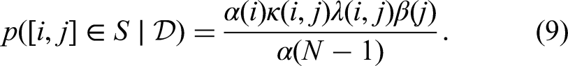
In addition, we can once again use the independence of data across arcs to get posterior marginals on each arc using

p ([i, j] \in S ∣ D) = \frac{α (i) κ (i, j) λ (i, j) β (j)}{α (N - 1)} .

(9)

Provided we have a specific model and algorithm that can yield the

κ (i, j)

for all relevant pairs, we can thus compute efficiently the posterior credences. The next subsection describes one such model.

Arc Model

The arc-level model is a standard Bayesian polynomial model, like the one in Bishop (2006), whose notation we largely borrow. The main difference in the approach is that we are not ultimately interested in the model parameters, but in the likelihood of the segment's data.

Throughout this section, we work under the assumption that there is an arc from index i to index j, with $j > i$ . To insulate the arc model from the global considerations, set $t = D [i, j]$ and $x$ as the normalized score time within the arc, that is,

x = {(\frac{k}{j - i})}_{k \in {0, \dots, j - i}} .

(10)

All variables defined in this section are then done so with respect to i and j, apart from the prior parameters

μ

Σ

and

η

, which are constant across all arcs.

First we assume that there is an ideal tempo series $y$ , representing the performer's intended tempo curve for the phrase, from which the observed data $t$ deviates by $ϵ$ . This deviation term is meant to encapsulate a variety of sources, such as finer-scale modulation (e.g., note-level rubato, beat annotation/extraction error, and execution error), and is modeled as independent, centered Gaussian noise, with a fixed variance $η$ as represented using

\begin{aligned} t = y + ϵ, \\ ϵ \sim N (0, η I), \end{aligned}

(11)

where

I

= identity matrix of the appropriate size.

We then model the ideal tempo as a quadratic function of score time, with independent Gaussian priors on its parameters using

\begin{matrix} y = Φ_{x} w, & (12) \\ w \sim N (μ, Σ), & (13) \\ Φ_{x} := [\begin{matrix} x_{0}^{2} & x_{0} & 1 \\ ⋮ & ⋮ & ⋮ \\ x_{N - 1}^{2} & x_{N - 1} & 1 \end{matrix}], & (14) \end{matrix}

where

x_{0}, \dots, x_{N - 1}

= individual values of x, μ and Σ, respectively, holding the means and (diagonal) covariance matrix of the priors on the quadratic, linear, and constant coefficients (in that order).

In summary, rewriting Equation 11 using Equation 12, we have that the distribution of $t$ given $w$ is

p (t ∣ w) = N (t | Φ_{x} w, η I)

(15)

which, marginalizing against

w

, yields

p (t ∣ w) = N (t | Φ_{x} μ, η I + Φ_{x} \sum {Φ_{x}^{}}^{T}) .

(16)

Inserting this formula as

κ (i, j)

into Equations 7 and 8, we can now proceed with the Bayesian updating of priors.

Output of the Proposed Model

In this section, we start with a brief description of the priors that we use in the computations for the remainder of this article and how they were set. We then show how the added complexity of the nuanced credence output can be handled through a few transformations and adequate visualizations. Finally, we comment on a few examples to exhibit how they can be used to extract knowledge about the performances.

Prior Setup

As always with Bayesian methods, the output is dependent on the priors. For the method, we need to select priors for likely segment lengths, phrase arc parameters, and noise.

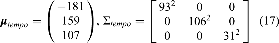
Tempo and loudness arc priors: in order to set reasonable priors, tempo and loudness arc boundaries were manually annotated for 37 performances across four pieces (initially 40, but three were discarded as the corresponding machine-generated beat annotations proved to be incorrect). Maximum likelihood estimates were then fitted to each arc in order to infer the corresponding model parameters, whose mean and variance were then used to construct the different priors. The resulting prior parameters were

μ_{t e m p o} = (\begin{matrix} - 181 \\ 159 \\ 107 \end{matrix}), Σ_{t e m p o} = [\begin{matrix} 93^{2} & 0 & 0 \\ 0 & 106^{2} & 0 \\ 0 & 0 & 31^{2} \end{matrix}]

(17)

η_{t e m p o} = 18.1, η_{l o u d} = 0.039,

(18)

μ_{l o u d} = (\begin{matrix} - 0.73 \\ 0.68 \\ 0.41 \end{matrix}), Σ_{l o u d} = [\begin{matrix} {0.55}^{2} & 0 & 0 \\ 0 & {0.60}^{2} & 0 \\ 0 & 0 & {0.19}^{2} \end{matrix}] .

(19)

We will demonstrate the model using tempo or loudness features. It is possible to run the model on both tempo and loudness features at once. However, as tempo and loudness variations are far from independent of each other, it is not sufficient to simply append their two priors; doing so leads to overconfident boundaries. Assuming independence between tempo and loudness leads to similar patterns in these features strongly reinforcing each other, whereas the reinforcement should be weak since the similarity is to be expected. Fixing this problem likely requires a more detailed setup of the covariance between features, which we leave for future work.

Segment length priors: for the prior on segment length, we have used a discretized Gaussian distribution, cut off at 30 beats, with mean 14.7 and standard deviation 5.95 (again set according to the 37 manual annotations).

These priors are wide, which is expected as the arcs can exhibit highly different shapes and expectations; priors that are too strict would likely result in poor segmentations. Overall, this means that posterior credences are mainly driven by the goodness of the arc fits, and that the priors only have a limited regularization role.

Visual Representations

Boundary credence can be readily visualized. They yield one real value per beat, similar to the input data, which can be plotted sequentially on the same graph, such as in Figure 2. An interesting complement to that information is to look at a moving window sum of the boundary credences. If the window is small enough, the corresponding boundaries are incompatible. For two close boundaries to coexist, there would need to be a very short segment between them, which would either fall below the minimum segment length or be extremely unlikely a priori, to the extent of being negligible. This means that the moving sum represents the posterior credence of having a boundary within that window.

Figure 2.

Tempo (red, upper curve), posterior boundary credence (solid blue) and its five-beat moving sum (dashed blue) for Csalog's interpretation of Mazurka 6-2. Background colors and letters reflect a reference score annotation by Witkowska-Zaremba (2000) (we divided their C section into C and C′ to keep segment lengths consistent).

This windowed sum could be used to reduce the nuanced output to a more familiar best guess of where boundaries are; for example, by selecting the peaks, on which the well-established segmentation evaluation techniques could be applied. In particular, this enables one to tune the guess directly to the level of tolerance used for the Boundary Hit Rate (Turnbull et al., 2007; Levy & Sandler, 2008).

Another use case of the moving sum is to easily distinguish boundaries that are almost certain, but for which there is still uncertainty about the exact location, from boundaries that are merely plausible, but could be optional as the two segments it delimits could be merged. Examples of the latter can be found around the mid-point of both B sections in Figure 2.

When looking at ambiguous structures, a richer view is to consider the posterior credences of segments, as they show how boundaries can chain together according to the alternative segmentations. However, they are harder to visualize efficiently and require some additional processing. In the next paragraphs, we shall introduce representations to visualize the segment credence outputs of the algorithm.

Segment credence matrix: a naive representation of the raw credence values for all possible segments is the segment credence matrix, $A_{i, j} = p ([i, j] \in S ∣ D)$ . However, this is simple but inefficient, as all nonzero values will be located close to the diagonal, with most of the matrix representing impossible segments [e.g., Figure 3(a)].

Figure 3.

Posterior segment credence for Csalog's interpretation of Mazurka 6-2: (a) raw segment credence matrix (A); (b) segment credence map (B, Eq. 20); (c) expanded segment credence map (C, Eq. 21); superimposed on the expanded credence map is a manual conversion of the map to a segmentation lattice, with bolder transitions being more credible. A candidate segment is highlighted throughout the different representations.

Segment credence map: the segment credence map is a first step toward an efficient representation by transforming the indexing from start and end position to start position and length of segment, that is

B_{i, j} = p ([i, i + j] \in S ∣ D) .

(20)

Here, B is essentially the same as A, but instead of indexing by the start and end positions of the arc, it is indexed by the start and length. An advantage of this transformation is that the values need only to be computed for acceptable segments. However, it may still be hard to see where each hypothetical segment ends. In addition, many values will still be practically null [Figure 3(b)].

Expanded segment credence map: we can take advantage of the segment credence map's sparsity by “spreading” each data point over its represented length to obtain the expanded segment credence map using

C_{i, j} = \sum_{k = 0}^{j} B_{i - j + k, j} .

(21)

An example of this expanded segment credence map is the background of the bottom representation in Figure 3. Since the summed probabilities are disjoint, this matrix has a strict interpretation, namely, each

(i, j)

value gives the probability that beat i is in a segment of length j. However, the insight from this representation comes not from its admittedly confusing definition but from visual inspection. One can think of each nonzero region as a possible segment: the greater the region's vertical span, the more uncertain its exact boundaries. Vertical region edges indicate sharp boundaries; sloped region edges mark uncertain boundaries.

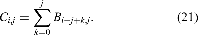
Segmentation lattice: the expanded segment credence map can be manually abstracted as a segmentation lattice, as shown superimposed on the representation in Figure 3(c). The lattice links pairs of segments that end and begin on successive beats. It provides an overview of the alternative segmentations, but discards information about the precise location of boundaries. Although the segmentation lattice was manually created in this case, its construction could likely be automated.

Musical Meaning of Outputs

Here, we discuss two sets of results of the segmentation extraction method. The first shows differences in interpretations of the same musical piece, and the second highlights the detection of expressive gestures in recorded performances.

Differences in Interpretations of the Same Musical Piece

Figure 4 shows the instantaneous tempo values and their derived boundary credence for Gbor Csalog's and Arthur Schoonderwoerd's interpretations of Chopin's Mazurka 06-2. The immediate observation is that, in both cases, boundaries are recovered where section changes occur; the remaining boundaries occur in the middle of sections, where a reference segmentation at a finer scale could have put boundaries. It is not surprising that the performances’ segmentations align well with a score-based segmentation, as the score's structure plays a large role in determining which patterns or groupings can be emphasized. There are nonetheless many differences between the segmentations projected by each performer.

Figure 4.

Computed boundary credence (in blue, lower curves) for interpretations of Mazurka 6-2 by: (a) Csalog; and (b and c) Schoonderwoerd. These are based on tempo (a and b) and loudness (c). The input data is shown in red (upper curves). Csalog makes more tempo boundaries than Schoonderwoerd. Csalog's extra boundaries tend to be in the middle of sections; Schoonderwoerd also marks these boundaries but through loudness.

In this instance, based on tempo, the model suggests that Csalog's performance mostly emphasizes four-bar groupings as seen in Figure 4(a), in contrast for example to Schoonderwoerd's performance, for which the four-bar groupings are visible in the raw data but are overshadowed by stronger eight-bar tempo arcs as shown in Figure 4(b). In the broader scheme, Schoonderwoerd also uses dynamics to demarcate four-bar subsections, as shown in Figure 4(c), which is picked up by the algorithm when run on loudness.

The output also shows that some boundaries are more precisely located than others. For instance, the position of the boundary around beat 168 is sharply defined to within a beat; whereas the next boundary, while still strongly detected overall, is spread out with a loosely defined location. This difference in boundary sharpness can also be observed between the tempo-based and loudness-based segmentations of Schoonderwoerd's performance, mainly due to the smoother nature of the loudness data in MazurkaBL. With smoother data, the Gaussian noise accounts for less of the variation, leading to tighter fits and thus more confident arc boundaries.

Another interesting feature of Csalog's performance is the weaker boundaries around beats 84, 132, and 156, none of which sum close to 1, reflecting some ambiguity in the structure. Indeed, Csalog weakly marks the four-bar groupings at these points, but the much higher prominence of the eight-bar arcs could justify skipping the lower-scale boundaries. This is very visible in the segmentation lattice in Figure 3(c), where the predominant path uses short segments for the A sections (except the one from beats 144 to 168) and long segments for the other sections, while still showing the alternative long and short sections, respectively.

Music Expressivity Visualized with Boundary Credence

Figure 5 shows the tempo-based output for two performances of Mazurka Op. 24-3: Rubinstein's 1966 recording and Fiorentino's recording. Interestingly, the resulting segmentations diverge from expert annotations while largely agreeing with one another.⁷ The explanation lies in the presence of tipping points (Chew, 2016b)—elongations of time for expressive effect—in the A sections. Where boundaries are detected correspond to mid-phrase fermate in the score. Indeed, there are tempo arcs starting and ending on these notes, but they arguably do not constitute phrase boundaries, and are in effect temporal tipping points. This result shows that the recovery of the interpreter's segmentation only works so long as the mapping between tempo (or loudness) arcs and musical groupings is not disrupted by other expressive effects. In this case, swapping out the arc model for another that would map correctly to the groupings could be envisioned. Nevertheless, it is interesting to recover expressive gestures such as tipping points, which are a form of musical thresholds.

Figure 5.

Temporal tipping points (suspensions of time flow for expressive effect) found in most performances of Mazurka 24-3 detected as peaks. Examples by: (a) Rubinstein 1966; and (b) Fiorentino. Reference sectional annotation by Witkowska-Zaremba (2000) shown in background (section C is a codetta rather than a proper section).

Manual comparison of posterior boundary and segment credences, as we have been doing in this section, is useful and can be enlightening, but it is unscalable to large databases such as MazurkaBL and its 2000 recordings for which tens of thousands of pairwise comparisons could be drawn, before even considering cross-piece and cross-feature comparisons. In the next section, we show how we can automatically grade the similarity between performed structures and identify where and how they differ.

Distance Based on Unbalanced Optimal Transport to Compare Boundary Credences

In this section, we propose a model to obtain similarities and differences between boundary credences. More precisely, we use unbalanced optimal transport to compute the proximity between the projected segmentations of two performances of the same piece. We then illustrate this method, first by applying it to one of the earlier examples, then systematically to large subsets of the MazurkaBL data set.

Unbalanced Optimal Transport-Based Distance Model

Motivation

With respect to the boundary credence of a given performance, a musician creating another performance may choose to make boundary credence peaks at different locations and with different shapes. For example, compared with Csalog's interpretation in Figure 4, Schoonderwoerd chose to create about half as many boundary credence peaks through tempo modulations, marking eight-bar-long phrases instead of four for Csalog. In addition, the peaks in Schoonderwoerd's interpretation have a different shape from those in Csalog's interpretation. Therefore, we propose to quantify the distance between two credence profiles by taking into account the possibility of having a different number of peaks and different shapes for each peak. The two different costs to be accounted for in the distance are:

Cost of deforming one peak into another: when peaks from boundary credence of two different interpretations are found at almost the same locations, they may be of different shapes, eliciting different perceptions from listeners. For example, the perception of a peak can change with a longer or shorter pause between two musical phrases.

Cost of destroying or creating peaks: when a peak is not matched in the comparative performance, this indicates different ways of grouping the music material. The presence or absence of peaks changes the locations and lengths of the musical phrases projected by the performer.

Consequently, each peak is deformed or destroyed and we choose to compute the distance between two boundary credences as the sum of the deformations of the matched peaks into one another and the unmatched peaks that are destroyed or created.

These deformations are computed based on unbalanced optimal transport that is a mathematical theory related to optimal transport (Monge, 1781; Kantorovich, 1942; Villani et al., 2009). Optimal transport studies how to transform points from a starting set to an ending set, while minimizing the total cost of transport, where the quantities of the starting and ending set are the same. Unbalanced optimal transport refers to a situation in which the quantities to be transported and the costs of transport are not balanced among the different sources and destinations. In our case, we are interested in moving the area under a boundary credence to the area under another boundary credence with minimal effort. However, we add the condition that the area under each peak can be transformed to at most one peak. This condition allows us to determine which peaks are similar or different between two boundary credences, which indicate the choices in the way the music is segmented through performance. This method based on unbalanced optimal transport is illustrated in Figure 6, and we mathematically formalize this distance in the next subsection.

Figure 6.

Illustration of the unbalanced optimal transport-based distance between two boundary credences f and $g$ . Solid red rectangles indicate matched peaks; dotted blue rectangles mark unmatched peaks.

Mathematical Formulation

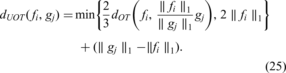
Let f and g be two boundary credences as represented in Figure 6. Each boundary credence normally comprises a series of peaks, that is, $f = {f_{i}}_{i \in I}$ and $g = {g_{j}}_{j \in J}$ , where I and J are indices of a set. We isolate the peaks within each boundary credence using a threshold set at $0.01$ —values above $0.01$ are part of some peak, and those below are not. We have found this value to be sufficient to isolate distinct peaks while discarding only negligible parts of the result. Regions above the threshold give the isolated peaks as illustrated in Figure 6 with $f = {f_{1}, f_{2}, f_{3}, f_{4}}$ and $g = {g_{1}, g_{2}, g_{3}}$ . Given $f_{i}$ a peak (which is a discrete function), recall that the distribution function $F_{i}$ of $f_{i}$ , and the area under the peak $∥ f_{i} ∥_{1}$ of $f_{i}$ are defined by

F_{i} (n) = \sum_{k = - \infty}^{n} f_{i} (k), ∥ f_{i} ∥_{1} = \sum_{k = - \infty}^{\infty} | f_{i} (k) | .

(22)

Let

f_{i}

and

g_{j}

be two peaks such that

∥ f_{i} ∥_{1} = ∥ g_{j} ∥_{1}

. The distance associated with discrete optimal transport⁸

d_{O T}

(Werman et al., 1985) between

f_{i}

and

g_{j}

, in the one-dimensional case, is written as

d_{O T} (f_{i}, g_{j}) = \sum_{n = - \infty}^{\infty} | F_{i} (n) - G_{j} (n) | .

(23)

From an algorithmic point of view, distribution functions can be readily computed, so it is straightforward to obtain the optimal transport distance between two peaks.

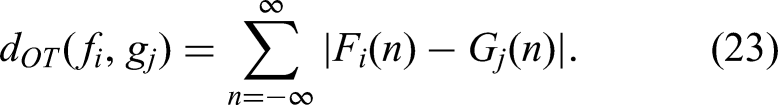
The two peaks may be temporally very distant, in which case it is preferable to destroy the area rather than move it. To do this, we use the unbalanced optimal transport (Chizat et al., 2018). Let $f_{i}$ and $g_{j}$ be two peaks such that $∥ f_{i} ∥_{1} = ∥ g_{j} ∥_{1}$ , we define the unbalanced optimal transport distance when peaks have the same area by

d_{U O T} (f_{i}, g_{j}) = min {\frac{2}{3} d_{O T} (f_{i}, g_{j}), ∥ f_{i} ∥_{1} + ∥ g_{j} ∥_{1}} .

(24)

According to this definition, if the minimum is

\frac{2}{3} d_{O T} (f_{i}, g_{j})

, it means that it is less costly to transform the area of one peak into another, but if the minimum is

∥ f_{i} ∥_{1} + ∥ g_{j} ∥_{1}

, it means that it is less costly to destroy the area of both peaks.

We now explain the $2 / 3$ factor. Because creating or removing a peak translates to a larger musical change than modifying the shape of a peak, we choose to reduce the modification cost between two peaks by a factor of $\frac{2}{3}$ . This factor means that it is as costly to match two identical peaks three beats apart with optimal transport as it is to destroy each of the peaks. In other words, the limit for deforming peaks is three beats, that is, one bar in case of Mazurkas. Mathematically, if $f_{i} = δ_{i^{'}}$ and $g_{j} = δ_{j^{'}}$ where $δ$ is the discrete dirac function (i.e., $δ_{i^{'}} (k) = 1$ if $k = i^{'}$ and $0$ elsewhere), then $d_{U O T} (f_{i}, g_{j}) = min (\frac{2}{3} | i^{'} - j^{'} |, 2)$ . Therefore, if $| i^{'} - j^{'} | > 3$ , that is, the two peaks are separated by more than three beats, then $d_{U O T} (f_{i}, g_{j}) = 2 = ∥ f_{i} ∥_{1} + ∥ g_{j} ∥_{1}$ , so it costs less to destroy both peaks than to deform one into the other. On the other hand, if $| i^{'} - j^{'} | < 3$ , that is, both peaks are less than three beats away, then $d_{U O T} (f_{i}, g_{j}) = \frac{2}{3} | i^{'} - j^{'} | = \frac{2}{3} d_{O T} (f_{i}, g_{j})$ and the cost of transforming one peak into the other is lower than destroying the peaks.

Finally, when two peaks, $f_{i}$ and $g_{j}$ , do not have the same area—for example, with $∥ f_{i} ∥_{1} \leq∥ g_{j} ∥_{1}$ —we scale the area of $g_{j}$ with the factor $\frac{∥ f_{i} ∥_{1}}{∥ g_{j} ∥_{1}}$ so that the two peaks have the same area and we add a term to signify the cost of the area lost, $∥ g_{j} ∥_{1} - ∥ f_{i} ∥_{1}$ , as already proposed by Gromov for the optimal transport formula when areas are different (Gromov et al., 1999, chapter 3 1/2, section B, p. 117). Suppose $f_{i}$ and $g_{j}$ are such that $∥ f_{i} ∥_{1} \leq ∥ g_{j} ∥_{1}$ , we define the distance associated with the unbalanced optimal transport between $f_{i}$ and $g_{j}$ by

\begin{aligned} d_{U O T} (f_{i}, g_{j}) = & min {\frac{2}{3} d_{O T} (f_{i}, \frac{∥ f_{i} ∥_{1}}{∥ g_{j} ∥_{1}} g_{j}), 2 ∥ f_{i} ∥_{1}} \\ + (∥ g_{j} ∥_{1} - ∥ f_{i} ∥_{1}) . \end{aligned}

(25)

Referring back to Figure 6, some f peaks are matched and moved to g peaks (solid red rectangles) and others are destroyed (dotted blue rectangle). Recall that each peak can only be matched once. We use a dynamic time warping algorithm to determine which peaks of f should be matched, or not, with those of g by allowing peaks to be matched with the zero-value function, which is equivalent to peak destruction. In Figure 6, the first peak

f_{1}

of f is slightly shifted toward the first peak

g_{1}

of g, the second peak

f_{2}

is deformed because it does not have the same shape as

g_{2}

, and the third peak

f_{3}

is destroyed because it does not match with any peak of g. In the end, the distance between two boundary credences is the sum of the cost of transforming or destroying each peak.

Revealing Similarities and Differences in Segmentations of Different Interpretations

We illustrate the distance based on unbalanced optimal transport using the Csalog's and Schoonderwoerd's interpretations of the Mazurka 6-2 shown in Figure 4. The comparison result is shown in Figure 7.

Figure 7.

Unbalanced optimal transport-based distance between the interpretation of the Mazurka 6-2 by Csalog and Schoonderwoerd. Note that the solid red rectangles indicating agreement tend to align with the annotated section boundaries, while dotted blue rectangles, the disagreements, typically mark more unusual boundaries. The right-most box contains both lines perfectly aligned.

In this figure, we can see which peaks are matched (marked by solid red rectangles) between the two performances and which peaks are removed (delineated with dotted blue rectangles). This can be useful for understanding the similarities and differences between two recorded performances. Because there are peaks between two successive sections in both performances (i.e., every eight bars), they are deformed into each other through unbalanced optimal transport. By contrary, most of the additional peaks of Csalog compared with Schoonderwoerd are destroyed. It is also interesting to notice that even if the second to last peaks of each performance are almost at the same time, they do not match. The algorithm prefers destroying them rather than deforming them because their shapes are too different. In addition, with respect to the last peak, the two curves are overlapped, so they cannot be distinguished in the figure and the peaks are matched with the unbalanced optimal transport-based distance (indicated by a solid red rectangle).

As a gauge of the credibility of our method's outputs, we compare the outputs to a known comparative analysis of recordings of Chopin's Mazurkas. Cook (2007) investigated the tempo variations of different recordings of the Mazurka 68-3, using correlations between the raw tempo curves of the different recordings and manually arranging them on a network to show the degrees of correlation between the recorded performances. This has been reproduced in Figure 8(a). Cook identified three clusters, thus three main ways of playing Mazurka 68-3 that he attributed in part to geographic location or teacher–pupil relationships between the different pianists. We automated the computation of a similar map from the same set of recordings of Mazurka 68-3, except for Fu T'song (not in our database).

Figure 8.

Similarity maps of interpretations of Chopin's Mazurka 68-3: (a) tempo-based correlation network manually created by Cook (2007); (b) automatically generated map based on unbalanced optimal transport distances between boundary credences.

We first computed the credence boundaries for each recording, then the distance between them based on the unbalanced optimal transport as described in the previous section. Finally, we automatically represent the results on a similarity map using the Python package manifold from the scikit-learn module (Pedregosa et al., 2011). The output is shown in Figure 8(b). We assigned a color to each of Cook's three clusters to highlight consistencies between this output and the analysis of Cook (2007). For example, observe that Rubinstein's interpretations are far from the average. In addition, there are other interpretations that are far from the average, as Cook noted, namely those of Ashkenazy, Biret, François, and Cortot.

Next, we apply the method to self similarity of interpretations of the Chopin mazurkas across multiple recordings by a performer. In the MazurkaBL database, Arthur Rubinstein stands out by far as the performer with the most recordings. He recorded three sets of mazurka performances: in 1939, 1952, and 1966. All three covered most, if not all, of the mazurkas. Although his style evolved over the years, his performances remained on average closer to his own than to that of others, according to our distance measure. Re-scaling the distance such that the closest performance pair on a piece is 0 and the farthest is 1, the average distance between Rubinstein's recordings of the same piece is 0.28, whereas that between Rubinstein's recording and another performer's is 0.52.

Extending this idea, it would seem reasonable to hypothesize that trends of proximity between artists can persist across pieces, perhaps due to similar grouping preferences or other similarities in their structural perception. To test this hypothesis, we focused on the subset of performers who recorded all of the mazurkas that Rubinstein recorded on all of his three sets (overall 30 mazurkas and 10 performers in addition to Rubinstein's three versions). We then looked at the 30 distance matrices for each mazurka, and proceeded to perform a Mantel test (Mantel, 1967) on each pair of mazurkas. However, only 39 of the 435 pairs showed significant correlation at the 5% level, which is higher than would be expected by chance, but far below what might result from a sizeable trend.

Conclusion and Future Work

We have described a method aimed at recovering the implicit segmentation conveyed through a musical performance. To achieve this, we have relied on a Bayesian framework, which has led to a nuanced output in which multiple segmentation hypotheses can co-exist. The method works on extracted prosodic features of an audio recording of a performance, without the need for score (note) information. The nuance acknowledges that with limited features and segmentation ambiguity, it may not be possible or desirable to have a precise localization of boundaries, and also that more than one segmentation can be a valid explanation for the observed data. To address the complexity introduced by this nuanced output, we have introduced the expanded segment credence map, which is a visualization of all plausible segmentations, including uncertainty about the precise position of segments’ endpoints.

We have shown on a selection of examples that this method finds segmentations that can reveal interesting structural differences between individual performances. There is some qualitative evidence that the performed structure could serve as a proxy for the score structure, which prompts further investigation such as using the algorithm's output as priors for estimating music structure (Smith & Goto, 2016). We have also proposed a comparison method based on unbalanced optimal transport that yields a distance between performed structures and highlights their similarities and dissimilarities. Interestingly, this distance revealed that Rubinstein's performed structures across the years were more similar to each other than those of other pianists. In contrast, we have found above chance but no significant correlation between two performers’ distance in one piece and their distance in another. This means that agreeing on performed structures in one piece may not imply agreement in another piece. However, it is important to recall that the comparisons mentioned have been based only on segmentations derived from tempo or loudness. Indeed, two performances can be similar in these aspects but may differ on other counts such as overall tempo or timbre.

In future work, it would be desirable to apply this method to a larger database of performances, preferably annotated with perceived structures. For example, the ASAP dataset (Foscarin et al., 2020) has a broader composer and piece range than the MazurkaBL dataset (Kosta et al., 2018b) we used, at the cost of a shallower range in performers. This broader range likely includes some pieces for which conventional interpretations do not exhibit the arching patterns we rely on, requiring a different segment model. Unfortunately, it still does not include performance structure annotations, and to our knowledge, neither does any currently available database, but projects such as CosmoNote (Fyfe et al., 2022) are in the process of assembling one.

A promising feature of the approach is that the two parts of the model are entirely decoupled. This means that the arc model could be improved—for example, to account for more features—without having to rework the overall model and algorithm. In addition, since the algorithm is agnostic of the recorded performance, the arc model could be entirely swapped out for a segment model suited to a different segmentation task.

We believe that, beyond the specifics of the model and algorithm presented, one of the key takeaways of this article is the choice of credence on boundaries or segments as outputs of segmentation. The credence-based approach has the potential to give deeper insights into music; for example, the distinction between (almost) certain or slightly plausible boundaries, and between strongly and weakly localized boundaries. In order to make full use of this rich output, new visualizations, tools, and methodologies will be critical. We have proposed a few, like the use of a moving sum to help distinguish between types of boundaries, but much remains to be done. Some of the most pressing questions in that pertaining to quantitative evaluation. A first, a relatively easy path would consist of condensing the nuanced output to best guesses in order to use existing methods and datasets, but a more rewarding path would see new methods embracing the uncertainty and ambiguity surrounding music segmentation.

In conclusion, given a recorded performance, we have shown how the performer's segmentation of the music material could be reverse engineered from the musical prosody through a computational Bayesian approach. The nuanced segmentation derived with our method provides insight into musicians’ understanding of the music, and the potential structure perceptions that could result from hearing the performance, thus also increasing the understanding of the experience of music. Finally, we have shown how the resulting boundary credence yields useful comparisons of musical interpretations using an optimal transport-based distance measure that compares favorably to intuition and manual analysis by a noted musicologist.

Supplemental Material

sj-pdf-1-mns-10.1177_20592043241233411 - Supplemental material for End-to-End Bayesian Segmentation and Similarity Assessment of Performed Music Tempo and Dynamics without Score Information

Supplemental material, sj-pdf-1-mns-10.1177_20592043241233411 for End-to-End Bayesian Segmentation and Similarity Assessment of Performed Music Tempo and Dynamics without Score Information by Corentin Guichaoua, Paul Lascabettes and Elaine Chew in Music & Science

Footnotes

Acknowledgments

This result is part of the project COSMOS that has received funding from the European Research Council under the European Union’s Horizon 2020 research and innovation program (grant number 788960). Paul Lascabettes is funded by a Contrat Doctoral Specifique pour Normaliens (CDSN) scholarship.

Action Editor

David Meredith, Department of Architecture, Design and Media Technology, Aalborg University, Aalborg, Denmark.

Peer Review

Adrián Barahona-Ríos, University of York, Department of Computer Science.

Kyle Worrall, University of York, Department of Computer Science.

Declaration of Conflicting Interests

The authors declared no potential conflicts of interest with respect to the research, authorship, and/or publication of this article.

Ethical Approval

This research did not require ethics committee or IRB approval. This research did not involve the use of personal data, fieldwork, or experiments involving human or animal participants, or work with children, vulnerable individuals, or clinical populations.

Funding

The authors disclosed receipt of the following financial support for the research, authorship, and/or publication of this article: This work was supported by the H2020 European Research Council (grant number 788960).

Supplemental Material

Supplemental material for this article is available online.

ORCID iDs

Corentin Guichaoua

Elaine Chew

Data Availability Statement

The MazurkaBL data set is available at https://github.com/katkost/MazurkaBL. Code for performing the probabilistic segmentation and its visualization is available at .

Notes

References

Bishop

C. M.

(2006). Pattern recognition and machine learning. Springer.

Cadwallader

(1998). Foreground motivic ambiguity: Its clarification at middleground levels in selected late piano pieces of Johannes Brahms. Music Analysis, 7(1), 59–91. https://doi.org/10.2307/939247

Chew

(2016a). From Sound to Structure: Synchronizing Prosodic and Structural Information to Reveal the Thinking Behind Performance Decisions. London International Piano Symposium, pp. 123–152.

Chew

(2016b). Playing with the edge: Tipping points and the role of tonality. Music Perception, 33(3), 344–366. https://doi.org/10.1525/mp.2016.33.3.344

Chew

(2023). Quantifying karajan. timing, dynamics and harmonic tension. Olms, pp. 25–41.

Chizat

Peyré

Schmitzer

Vialard

F.-X.

(2018). Scaling algorithms for unbalanced optimal transport problems. Mathematics of Computation, 87(314), 2563–2609. https://doi.org/10.1090/mcom/3303

Chuan

C. H.

Chew

(2007). A dynamic programming approach to the extraction of phrase boundaries from tempo variations in expressive performances. In Proceedings of the 8th International Society for Music Information Retrieval Conference (ISMIR), pp. 305–308, Vienna, Austria.

Clarke

(2005). Music, Motion and Subjectivity. Oxford University Press, pp. 62–90.

Cook

(2007). Performance analysis and Chopin’s Mazurkas. Musicae Scientiae, 11(2), 183–207. https://doi.org/10.1177/102986490701100203

10.

Cook

(2014). Between art and science: Music as performance. Journal of the British Academy, 2, 1–25. https://doi.org/10.5871/jba/002.001

11.

Degara

Argones Rua

Pena

Torres-Guijarro

Davies

Plumbley

(2011). Reliability-informed beat tracking of musical signals. IEEE Transactions on Audio, Speech and Language Processing, 20(1), 290–301. https://doi.org/10.1109/TASL.2011.2160854

12.

Fastl

(2005). Psycho-Acoustics and Sound Quality. Springer Berlin Heidelberg, pp. 139–162.

13.

Fearnhead

Liu

(2011). Efficient Bayesian analysis of multiple changepoint models with dependence across segments. Statistics and Computing, 21(2), 217–229. https://doi.org/10.1007/s11222-009-9163-6

14.

Foscarin

McLeod

Rigaux

Jacquemard

Sakai

(2020). ASAP: a dataset of aligned scores and performances for piano transcription. In International Society for Music Information Retrieval Conference (ISMIR), pp. 534–541.

15.

Fyfe

Bedoya

Chew

(2022). Annotation and analysis of recorded piano performances on the web. Journal of the Audio Engineering Society, 70(11), 962–978. https://doi.org/10.17743/jaes.2022.0057

16.

Gabrielsson

(1987). Once again: The theme from Mozart’s piano sonata in A major (K.331). Action and perception in rhythm and music, pp. 81–103.

17.

Gody

R. I.

Jensenius

A. R.

Nymoen

(2010). Chunking in music by coarticulation. Acta Acustica United with Acustica, 96(4), 690–700. https://doi.org/10.3813/AAA.918323

18.

Gromov

Katz

Pansu

Semmes

(1999). Metric structures for Riemannian and nonRiemannian spaces. Vol. 152. Springer.

19.

Guichaoua

(2017). Modèles de compression et critères de complexité pour la description et l’inférence de structure musicale [Phd thesis]. Université Rennes 1.

20.

Haralick

R. M.

Shapiro

L. G.

(1985). Image segmentation techniques. Computer Vision, Graphics, and Image Processing, 29(1), 100–132. https://doi.org/10.1016/S0734-189X(85)90153-7

21.

Kantorovich

L. V.

(1942). On the translocation of masses. In Dokl. Akad. Nauk. USSR (NS), Vol. 37, pp. 199–201.

22.

Koprinska

Carrato

(2001). Temporal video segmentation: A survey. Signal Processing: Image Communication, 16(5), 477–500. https://doi.org/10.1016/S0923-5965(00)00011-4

23.

Kosta

Bandtlow

Chew

(2018a). Dynamics and relativity: Practical implications of dynamic markings in the score. Journal of New Music Research, 47(1), 1–24. https://doi.org/10.1080/09298215.2018.1486430

24.

Kosta

Bandtlow

O. F.

Chew

(2018b). MazurkaBL: Score-aligned Loudness, Beat, and Expressive Markings Data for 2000 Chopin Mazurka Recordings. Proceedings of the International Conference on Technologies for Music Notation and Representation – TENOR’18, pp. 85–94.

25.

Kosta

Ramrez

Bandtlow

Chew

(2016). Mapping between dynamic markings and performed loudness: A machine learning approach. Journal of Mathematics and Music, 10(2), 149–172. https://doi.org/10.1080/17459737.2016.1193237

26.

Langner

Goebl

(2003). Visualizing expressive performance in tempo-loudness space. Computer Music Journal, 27(4), 69–83. https://doi.org/10.1162/014892603322730514

27.

Lascabettes

Agon

Andreatta

Bloch

(2022a). Computational Analysis of Musical Structures based on Morphological Filters. In International Conference on Mathematics and Computation in Music, Atlanta, GA, USA.

28.

Lascabettes

Guichaoua

Chew

(2022b). Generating multiple hierarchical segmentations of music sequences using adapted correlative matrices. In Proceedings of the 19th Sound and Music Computing Conference, page In press, Saint Etienne, France.

29.

Leech-Wilkinson

(2017). Musical Shape and Feeling. Oxford Academic Books, pp. 359–382.

30.

Levy

Sandler

(2008). Structural segmentation of musical audio by constrained clustering. IEEE Transactions on Audio, Speech, and Language Processing, 16(2), 318–326. https://doi.org/10.1109/TASL.2007.910781

31.

Lewin

(2007). Musical Form and Transformation: Four Analytic Essays. Oxford Academic Bookx.

32.

Mantel

(1967). The detection of disease clustering and a generalized regression approach. Cancer Research, 27(2 Part 1), 209–220.

33.

Mazzola

(2011). Musical Performance – A Comprehensive Approach: Theory, Analytical Tools, and Case Studies. Springer.

34.

Monge

(1781). Mémoire sur la théorie des déblais et des remblais. Mem. Math. Phys. Acad. Royale Sci., pp. 666–704.

35.

Nieto

Mysore

G. J.

Wang

C.-i.

Smith

J. B.

Schlüter

Grill

McFee

(2020). Audio-Based music structure analysis: Current trends, open challenges, and applications. Transactions of the International Society for Music Information Retrieval, 3(1), 246–263. https://doi.org/10.5334/tismir.78

36.

Palmer

Hutchins

(2006). What is musical prosody? Psychology of Learning and Motivation, 46, 248–278. https://doi.org/10.1016/S0079-7421(06)46007-2

37.

Paulus

Müller

Klapuri

A. P.

(2010). Audio-Based Music Structure Analysis. In Proceedings of the 11th International Society for Music Information Retrieval Conference (ISMIR), number Ismir, pp. 625–636.

38.

Pedregosa

Varoquaux

Gramfort

Michel

Thirion

Grisel

Duchesnay

(2011). Scikit-learn: Machine learning in Python. Journal of Machine Learning Research, 12(85), 2825–2830. https://dl.acm.org/doi/10.5555/1953048.2078195

39.

Rigaill

Lebarbier

Robin

(2012). Exact posterior distributions and model selection criteria for multiple change-point detection problems. Statistics and Computing, 22(4), 917–929. https://doi.org/10.1007/s11222-011-9258-8

40.

Rink

(1995). Playing in time: Rhythm, metre and tempo in Brahms’s Fantasien Op. 116. Cambridge University Press, pp. 254–282.

41.

Rupprecht

Laina

Dipietro

Baust

Tombari

Navab

Hager

G. D.

(2017). Learning in an Uncertain World: Representing Ambiguity Through Multiple Hypotheses. In Proceedings of the IEEE International Conference on Computer Vision, pp. 3611–3620, Venice, Italy.

42.

Sakran

A. E.

Abdou

S. M.

Hamid

S. E.

Rashwan

(2017). A review: Automatic speech segmentation. International Journal of Computer Science and Mobile Computing, 6(4), 308–315.

43.

Sargent

Bimbot

Vincent

(2017). Estimating the structural segmentation of popular music pieces under regularity constraints. IEEE/ACM Transactions on Audio, Speech, and Language Processing, 25(2), 344–358. https://doi.org/10.1109/TASLP.2016.2635031

44.

Smith

Goto

(2016). Using Prior to Improve Estimates of Music Structure. In International Society for Music Information Retrieval Conference, New York, NY, USA.

45.

Smith

J. B.

Chew

(2017). Automatic interpretation of music structure analyses: A validated technique for post-hoc estimation of the rationale for an annotation. In Proceedings of the 18th International Society for Music Information Retrieval Conference, ISMIR 2017, pp. 435–441, Suzhou, China.

46.

Smith

J. B.

Schankler

Chew

(2014). Listening as a creative act: Meaningful differences in structural annotations of improvised performances. Music Theory Online, 20(3). https://doi.org/10.30535/mto.20.3.3

47.

Stowell

Chew

(2013). Maximum a posteriori estimation of piecewise arcs in tempo time-series. In Aramaki

Barthet

Kronland-Martinet

Ystad

(Eds.), From sounds to music and emotions (pp. 387–399). Springer.

48.

Temperley

. (2007). MIT Press, Cambridge, MA, USA.

49.

Todd

N. P. M.

(1992). The dynamics of dynamics: A model of musical expression. Journal of the Acoustical Society of America, 91(6), 3540–3550. https://doi.org/10.1121/1.402843

50.

Turnbull

Lanckriet

G. R. G.

Pampalk

Goto

(2007). A Supervised Approach for Detecting Boundaries in Music Using Difference Features and Boosting. In Proceedings of the 8th International Society for Music Information Retrieval Conference (ISMIR), pp. 51–54, Vienna, Austria.

51.

Villani

, et al. (2009). Optimal transport: old and new. Vol. 338. Springer.

52.

Wang

C.-i.

Gautham

J. M.

Dubnov

(2017). Re-Visiting the Music Segmentation Problem With Crowdsourcing. In Proceedings of the 18th International Society for Music Information Retrieval Conference (ISMIR), pp. 738–744, Suzhou, China.

53.

Werman

Peleg

Rosenfeld

(1985). A distance metric for multidimensional histograms. Computer Vision, Graphics, and Image Processing, 32(3), 328–336. https://doi.org/10.1016/0734-189X(85)90055-6

54.

Widmer

Tobudic

(2003). Playing mozart by analogy: Learning multi-level timing and dynamics strategies. Journal of New Music Research, 21(1), 259–268. https://doi.org/10.1076/jnmr.32.3.259.16860

55.

Witkowska-Zaremba

(2000). Versification, Syntax and Form in Chopin’s Mazurkas. Polish Music Journal, 3(1).

56.

Zacks

J. M.

Swallow

K. M.

(2007). Event segmentation. Current Directions in Psychological Science, 16(2), 80–84. https://doi.org/10.1111/j.1467-8721.2007.00480.x

Supplementary Material

Please find the following supplemental material available below.

For Open Access articles published under a Creative Commons License, all supplemental material carries the same license as the article it is associated with.

For non-Open Access articles published, all supplemental material carries a non-exclusive license, and permission requests for re-use of supplemental material or any part of supplemental material shall be sent directly to the copyright owner as specified in the copyright notice associated with the article.

0.00 MB

0.10 MB