
Abstract
Despite the existing evaluation of the sampling options for periodical media content, only a few empirical studies have examined whether probability sampling methods can be applicable to social media content other than simple random sampling. This article tests the efficiency of simple random sampling and constructed week sampling, by varying the sample size of Twitter content related to the 2014 South Carolina gubernatorial election. We examine how many weeks were needed to adequately represent 5 months of tweets. Our findings show that a simple random sampling is more efficient than a constructed week sampling in terms of obtaining a more efficient and representative sample of Twitter data. This study also suggests that it is necessary to produce a sufficient sample size when analyzing social media content.
Individuals’ daily activities are increasingly logged and transformed into large-scale datasets. As these digital traces, particularly digitally exchanged information via social networking sites (SNSs) and even online news content, have become readily available, social scientists have endeavored to analyze such media content. Researchers have used social media data to predict election results (Anstead & O’Loughlin, 2014; Gayo-Avello, 2013), detect the outbreak of influenza (Ginsberg et al., 2008), and estimate the revenue of released films (Mestyan, Yasseri, & Kertesz, 2013).
There are two types of methodological approaches to social media analysis. Some take a big-data approach, analyzing literally all existing content (Colleoni, Rozza, & Arvidsson, 2014; Neuman, Guggenheim, Jang, & Bae, 2014). This approach does not involve the traditional sampling process. Instead, it relies on keyword-based or automated computational analysis. The problem of this approach, however, is that complex variables and nuanced texts are not efficiently identified or meaningfully categorized because of the use of nonhuman tools (Zamith & Lewis, 2015). Second, the computational analysis often uses an algorithm for coding. Sometimes, data researchers may not realize the high sensitivity of the conceptual boundaries of topics and the sampling frames of large-scale data under examination. Because reliability is a necessary but not sufficient requirement for validity, they need to demonstrate the validity of algorithms by comparing the results from two different algorithms. In many cases, however, this process has often been omitted. In addition, it is hard to measure the descriptive statistics of certain thematic writing components, such as frames. Thus, depending on the purpose of the study, others take a human coding approach using a traditional sampling process, which is the subject of this article.
A substantial body of literature has tested the efficiency of different types of sampling methods with traditional mass media content. This includes daily and weekly newspapers, weekly and monthly news magazines, broadcast news, and online news (Hester & Dougall, 2007; Lacy, Riffe, & Randle, 1998; Lacy, Robinson, & Riffe, 1995; Riffe, Aust, & Lacy, 1993; Riffe, Lacy, & Drager, 1996; Riffe, Lacy, Nagovan, & Burkum, 1996). These studies have almost exclusively focused on periodical media outlets in which the volume and nature of media content are largely influenced by periodical variations in advertising and information gathering that affect space and time available for content (Riffe et al., 1993). For example, news articles published on weekdays and weekends are substantially different from each other in many aspects (Neuman et al., 2014). To minimize systematic errors, researchers have suggested that a content sampling technique should consider or control for such cyclical variations (Luke, Caburnay, & Cohen, 2011; Riffe et al., 1993).
While the extant literature has focused on the sampling process of periodical media content, whether the traditional sampling technique is applicable to social media data is largely under-explored. Although mass media content has been heavily constrained by its limited carrying capacity, social media provide almost unlimited time and space for both content providers and consumers. Users can generate social media content without being constrained by a news hole or broadcast schedule. Thus, the daily volume of social media content fluctuates in a more unexpected fashion and may not clearly show cyclical trends. Given the different nature of social media content, it is imperative that scholars not only evaluate existing sampling methods but also look for an alternative approach for the sampling procedure of social media content.
We address this issue by applying existing media sampling options to Twitter data in the context of the 2014 South Carolina gubernatorial election. This study assesses two established sampling techniques—simple random sampling (SRS) and constructed week sampling—varying the sample size of the Twitter content. In addition, we explore how many days or weeks are needed to adequately represent a given time period.
Literature Review
Traditional Sampling Methods
To conduct a content analysis of traditional media, various sampling options have been considered. Probability or random sampling is based on the assumption that each item of a certain population is given an equal chance to be selected in the sample (Riffe, Lacy, & Fico, 2005). For example, if certain key terms more frequently appear in the population, they will be more often found in the sample as well. This probability sampling can be justified “because of the laws of probability” (Riffe et al., 2005, p. 103). Most research on traditional media has tested three types of sampling procedures: SRS, constructed week sampling, and consecutive day sampling. SRS—or its modified version, systematic sampling—means the technique to randomly select a sample from a population. Thus, each sample in the population has an equal chance to be selected (Riffe et al., 2005). However, if the population list is not easily attainable or the list is too long, other sampling methods should be suggested (Riffe et al., 2005).
Constructed week sampling is one type of stratified sampling method. This technique samples media content based on the day of the week. For example, Monday news articles are sampled within a pool of Monday news articles, and Tuesday articles are samples within a pool of Tuesday articles. In this way, a researcher can construct a week or several weeks that represent all days of the week. Previous studies have indicated that constructed week sampling can reduce the possibility of overestimating or underestimating certain days of the week (Riffe et al., 1993).
Finally, consecutive day sampling refers to the method to select a convenience sample of 7 or more than 7 consecutive days. This sampling method is particularly convenient to use, but it is not considered as a reliable way of analyzing content for a period of 6 months or longer (Riffe et al., 1993). Overall, research on traditional media sampling has tested the efficiency of these three sampling methods, and reported that constructed week samples tend to produce more efficient estimates than simple random or consecutive day samples (Hester & Dougall, 2007; Lacy et al., 1995; Riffe et al., 1993; Riffe et al., 1996).
Different Nature of Social Media Data
As Kim et al. (2013) noted, sampling approaches of a large-scale dataset, such as Twitter, should be different from those of traditional media. This may be due to the characteristics of social media, which are free from some of the traditional constraints. Previously, the amount of mass media content produced was typically constant within a certain period because of the limits of disseminating space and organizational resources. Regardless of how insignificant a day’s events may be, news organizations must fill the full day with news stories. Even when breaking news changes routines and requires resource reallocations, it is unlikely that the size of the news hole becomes much bigger (Bennett, 1990; Ryfe, 2006). However, in social media, there are no limits on production and broadcasting capacity. As a result, social media display a flexible nature, operating 24 hr continuously with almost an unlimited number of content providers. Importantly, large-scale social media data do not show daily or weekly cycle variations, which are a key characteristic of traditional media content. Neuman et al. (2014) found that although both traditional and social media show a weekly cycle in which the amount of content is lower on weekends, the tendency is much more clearly observed in traditional media than in social media. Besides, social media content does not always show this weekly cycle, but varies depending on the topic. For example, tweets about entertainment topics are produced more over weekends than during weekdays. On the other hand, this reverse cycle is not shown in traditional news stories.
Traditional sampling methods often use a day as a unit of analysis, and researchers select certain days and automatically include all stories that are published in those days. Thus, previous sampling methods focus on the way in which researchers efficiently select representative days, assuming that the amount of news content will be quite consistent across different days. However, this approach may not be appropriate to social media because a daily volume of social media content can fluctuate significantly. Therefore, this method is highly vulnerable to the possibility of under- or overestimating the content volume. In addition, depending on the topic of interest, it is possible that certain days do not show any tweets. If such days are selected through a traditional sampling approach, the frequencies of certain variables can necessarily be underestimated.
Sampling Social Media Content
Although there is little consensus on how to draw a sample from a large-scale social media data (Lewis, Zamith, & Hermida, 2013), a number of studies have analyzed social media content using datasets sampled one way or another. Exploring the number of tweets mentioning key political parties, for example, Tumasjan, Sprenger, Sandner, and Welpe (2010) successfully predicted the 2009 German federal election results. However, raising two aspects of concern about Tumasjan et al.’s (2010) study—arbitrary selection of parties as samples and questionable choice of the sampling time frame, Jungherr, Jürgens, and Schoen (2012) criticized that Tumasjan et al.’s article could not warrant the prediction of the German federal elections. Subsequently Tumasjan, Sprenger, Sandner, and Welpe (2012) refuted Jungherr et al.’s claims, arguing that their original manuscript was well supported by both selection of Twitter data and the sampling time frame. This debate shows an analytic problem in social media content research including Twitter data.
Depending upon the purpose of studies and the characteristics of the datasets, researchers have employed several different sampling techniques. These sampling methods can be categorized into three approaches. First, some researchers used SRS to produce a study sample (e.g., Cavazos-Rehg et al., 2016; Chew & Eysenbach, 2010; Giglietto & Selva, 2014; Takahashi, Tandoc, & Carmichael, 2015). For example, Takahashi et al. (2015) collected tweets regarding Typhoon Haiyan between 8 and 13 November 2013 by searching tweets at three different time points each day. Then they created a study sample by taking a simple random sample of 1,000 tweets. Using SRS, Cavazos-Rehg et al. (2016) also content-analyzed tweets on depression. Using a keyword search, the researchers collected all tweets between 11 April and 4 May 2014, and then randomly selected 2,000 tweets from the pool of identified depression-related tweets.
Other researchers used constructed week sampling (e.g., Artwick, 2014; Giglietto & Selva, 2014; Harlow & Johnson, 2011). To analyze tweets posted by newspaper reporters, for example, Artwick (2014) randomly selected one Monday from all available Mondays between 1 April and 30 June 2011, one Tuesday from all available Tuesdays, and all other remaining days, using the same methods. Then, a total of 2,733 tweets were selected from the constructed 1 week. Harlow and Johnson (2011) also used constructed week sampling to analyze traditional and social media content on the 2011 Egyptian democratic movement. The researchers examined three types of media contents: the New York Times stories, tweets of a Times reporter, Nick Kristof, and posts on the citizen media site, Global Voice. A total of 208 stories were selected, using a constructed week sample between 23 January and 14 February, 2011. Because their study compared tweets and news in traditional media, it might require a mixed sampling plan.
Researchers also used convenience sampling for a social media content analysis according to their purposes (e.g., Adams & McCorkindale, 2013; Clark & Ferguson, 2011; Waters & Jamal, 2011). For example, Clark and Ferguson (2011) examined how local television used Twitter for promotion and branding. They first searched local television stations that managed Twitter sites on 25 September 2009, and found a total of 488 stations. They selected only the first page of each television station account because of the high volume of postings on sites.
Although numerous studies evaluate sampling options for traditional media content including periodicals and broadcasting newscasts, little is known about how to sample a large-scale dataset such as Twitter and Facebook. In a few examples where researchers have used randomly selected samples and constructed week samples (e.g., Chew & Eysenbach, 2010; Harlow & Johnson, 2011), they have relied on studies from traditional media to guide sampling approaches. However, a question that remains is whether the same sampling strategies are efficiently applicable to social media content. Is social media content affected by cyclic variations similar to periodical mass media content? If not, do we still need to consider errors caused by weekday variations? Thus, this study addresses this issue by testing the efficiency of existing sampling methods with Twitter data.
RQ1. Is a constructed week sample more efficient than a simple random sample of comparable size when examining a dataset of Twitter content?
RQ2. What is the minimum number of weeks needed to accurately generalize to a population of 5 months of tweets?
Methods
Data Source
To test the efficiency of different sampling options, we compare sample statistics obtained from the different sampling options against population parameters. Thus, the population size should be manageable to the extent that human coders conduct the manual coding for all population tweets. Given this consideration, this study focused on tweets about the 2014 South Carolina gubernatorial election. The dataset included tweets about the 2014 South Carolina gubernatorial election from 10 June 2014 to 3 November 2014. We selected this time period because 10 June was the primary election day and 3 November was the day before the general election in South Carolina. Tweets were retrieved using a Boolean keyword search of the Sysomos database. The third-party licensed firm Sysomos provided Twitter data. As Twitter’s open access policy via application programming interface (API) has been increasingly restricted, it is necessary to work with a firm such as Sysomos to capture the entire archive of Twitter posts. As our data were free from “spam” tweets (i.e., Twitter bots), the retrieved data for this study indicate active accounts held by real users.
Using the 2014 South Carolina gubernatorial election as a population parameter, we included all tweets that mentioned both candidate names and election-related words: (“Nikki,” OR “Haley,” OR “Vincent,” OR “Vince,” OR “Sheheen”) AND (“election,” OR “candidate,” OR “campaign,” OR “governor,” OR “gubernatorial.”). Our search yielded a total of 1,968 tweets. Note that the purpose of this study is to compare sampled tweets with predetermined population tweets. Whether searched population tweets represent all tweets about the gubernatorial election does not undermine this goal.
The topic and volume of tweets can be volatile compared with traditional media content. For example, as our population tweets are all related with the gubernatorial election, many more tweets than the average were generated immediately before Election Day. By comparison, the fourth week of our population tweets yielded very few tweets. Thus, if a day having a very small number of tweets is chosen, sampled, and examined, an analysis with that sample may be increasingly vulnerable to sampling error. Thus, this study excluded days producing less than five daily tweets. After excluding 72 tweets, we finally analyzed a total of 1,896 tweets out of the 107 days.
Coding Procedure
After a series of training, two coders explored each of the 1,968 tweets collected during the 21-week period. This study used 10 variables, including 3 basic information variables, 5 election frame variables, and 2 tones of candidate variables. First, as basic information variables, we examined and coded whether a tweet had a link to other webpages, whether a tweet was retweeted, and whether a tweet showed any photograph or video footage. By comparing the percentage of presence of these basic variables between sampled and population tweets, we can assess the representativeness of various sampling methods.
Next, we further compared various sampling options using more sophisticated variables that involve subjective characteristics. Following the literature of campaign news themes (Jang & Oh, 2016; Lichter, 2001), we categorized election-related posts into five election frames, including horserace, issue, candidate, campaign trail, and voter. Each variable was nominally coded as presence or absence. The horserace frame involves talking about poll results, winning and losing status, and tactics to increase favorable votes. The issue frame discusses national or local issues or candidates’ policy positions such as healthcare, immigration, and local development. The candidate frame concerns candidates’ personalities, political abilities, leadership styles, and family matters. The campaign trail frame includes campaign events such as candidate speeches, visits, meetings, and future campaign events. The voters frame focuses on individual voters’ reactions to candidates or campaigns. These variables were coded initially as presence or absence as nominal variables, and then for the subsequent comparison procedure, recoded into the percentage of presence each day (see Hester & Dougall, 2007; Lacy et al., 1995; Riffe et al., 1993).
Finally, we used the tone of two candidates—Nikki Haley and Vincent Sheheen—as one of our variables to be compared. Because some tweets mention both candidates, we coded the tone of each candidate separately. Tone was coded as an ordinal category by classifying 1 to a negative, 2 to a neutral, and 3 to a positive tweet. Thus, tone is regarded as an ordinal variable. If the candidates were not mentioned in a tweet, the tweets were excluded only for the analysis of the tone variables.
Intercoder reliability was calculated by double-coding a random subsample (n = 311 or 15.8%) of the data. Intercoder reliability corrected for agreement by chance (Krippendorff’s alpha) ranged between .80 and .96 with an average reliability of .90. 1
Evaluation procedure
This study followed the comparison procedure suggested by previous research that tested the efficiency of constructed week and SRS methods (Hester & Dougall, 2007; Lacy et al., 1995; Riffe et al., 1993; Riffe et al., 1996). Some studies also evaluated the consecutive day sampling, but none of them recommended this technique. Thus, we did not test the consecutive day sampling method.
The procedure of evaluation, when the unit of analysis is each day, is described as follows: (1) obtain population mean and standard errors for each target variable, (2) use constructed week and SRS methods and draw 100 sets of one constructed week (n = 7) and random 7 days (n = 7), and (3) count the number of sets (out of 100) whose mean values fall within plus or minus one standard error of the population mean. If we observe more sets to meet this condition, we can consider the sampling strategy more efficient. This process illustrates the case in which one constructed week samples (n = 7) and randomly selected 7-day samples (n = 7) are compared. To make comparisons with a greater sample size, we continued to draw separate 100 samples until 10 constructed weeks (n = 70) and random 70 days were drawn. With this process, we can determine the minimum number of weeks needed to accurately represent population tweets.
Using each tweet as a unit of analysis involves slightly different processes. We first need to draw a comparable sample size. It should be noted that the number of sampled tweets varies when each day is used as a unit of analysis. This is because each day or week produces a different number of tweets. When studying traditional media content, this daily or weekly variation was considered trivial and conveniently ignored. However, we question this assumption. According to our population dataset, each week generated 124 tweets on average. As mentioned above, we excluded days generating less than five daily tweets. The average tweet number was calculated including all days and weeks because less than five daily tweet days are a legitimate part of the population. Thus, we considered that 124 tweets were corresponding to one constructed week samples or randomly selected 7-day samples.
To generate constructed week samples using each tweet as a unit of analysis, we calculate the average number of tweets for each day of the week. For example, Mondays averagely produced 14 tweets, while Sundays produced 6 tweets on average. Using this calculation, we proportionally draw 100 sets of one constructed week consisting of 124 tweets. For SRS, we draw 100 sets of 124 randomly selected tweets without considering day of the week differences. Again, to make comparisons with greater sample size, we continued to draw separate 100 samples until 10 constructed weeks (n = 1,240 tweets) and randomly selected 1,240 tweets were drawn.
Thus, finally, we evaluated the efficiency of two sampling methods (constructed week sampling and SRS) and sample sizes (ranging between 1 and 10 weeks or 124 and 1,240 tweets). Following the previous literature (Hester & Dougall, 2007; Lacy et al., 1995; Riffe et al., 1993; Riffe et al., 1996), a series of assessments were made by measuring how often sample means fell within one standard error of the population mean. 2
Results
Before examining our primary research questions, Table 1 presents the population mean, population standard deviation, and coefficient of variation (CV) for each variable and each unit of analysis. It should be repeated that nominal variables were recoded into percentage values and the two ordinal variables remained the same. The CV refers to the standard deviation divided by the mean (Hester & Dougall, 2007). We included CV values because they can inform how each unit is varied in the population, suggesting that a higher CV shows more variation and a lower CV indicates less variation.
Population Distribution.
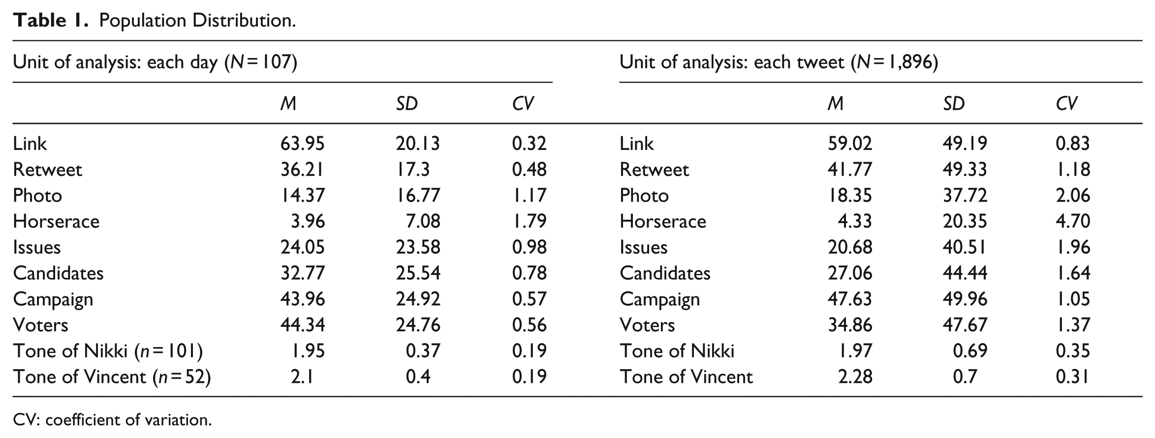
CV: coefficient of variation.
The first research question asked the efficiency of constructed week and random sampling methods. To answer this, we compared the percentages of means in each set of 100 simple random samples and constructed week samples that were within plus or minus one standard error of the population. Table 2 shows the results for 100 samples of 10-week samples for when a unit of analysis is each day or each tweet. Each underlined percentage indicates that the sampling percentage met the critical values determined by the Central Limits Theorem (68% for plus or minus one standard error; Hester & Dougall, 2007; Lacy et al., 1995; Riffe et al., 1993; Riffe et al., 1996).
The Percentage of 100 Samples Where the Sample Mean Falls Within Plus or Minus 1 Standard Error of the Population Mean by Type and Size of Sample for 10 Variables.

The Central Limits Theorem predicts that 68% will be within plus or minus one standard error of the population mean. The underlined percentages mean the sampling percentages that exceed this critical value. Nominal variables include Link, Retweet, Photo, Horserace, Issues, Candidate, Campaign, and Voter. Ordinal variables indicate Tone of Nikki and Tone of Vincent.
When comparing constructed week and SRS methods, simple random samples appeared to show a greater level of efficiency. This pattern was obvious when the unit of analysis is each day. For simple random samples, 23 samples of nominal variables and 7 samples of ordinal variables met the critical standard. However, for constructed week samples, only four samples of nominal variables and five samples of ordinal variables met the decision standard. For nominal variables, the distribution of samples that exceeded the critical value (68%) showed a significant difference between simple random samples and constructed week samples (χ2 = 95.00, p < .01). For ordinal variables, however, the distribution of samples that met the critical value did not show a significant difference between simple random samples and constructed week samples (χ2 = 1.07, p = ns).
On the other hand, when a unit of analysis was each tweet, both distributions of nominal and ordinal samples that met the critical value did not indicate a significant difference between simple random samples and constructed week samples (χ2 = .06, p = ns; χ2 = .00, p = ns). A total of 25 samples of nominal variables and 9 samples of ordinal variables met the decision standard, while 24 samples of nominal variables and 9 samples of ordinal variables met the critical value for constructed week samples. These results indicate that simple random samples are more efficient than constructed week samples when a unit of analysis is each tweet and variables are measured as nominal.
Our second research question asked was what was the minimum number of weeks needed to accurately generalize to a population of 5 months of tweets? Because our findings indicate that SRS is the most efficient technique when a unit of analysis is each tweet, we look at the minimum number of weeks only when using SRS for each tweet. Previous studies suggest that the sample size is reasonably efficient when its percentages equaled or exceeded the expected percentages (Hester & Dougall, 2007; Riffe et al., 1993). As Table 1 shows, a sample of 7 weeks was efficient for Link (CV = .83) and Issues (CV = 1.96), and a sample of 8 weeks was efficient for seven variables. As for two ordinal variables, a sample of 6 weeks was efficient for Tone of Vincent (CV = .31) and a sample of 7 weeks was efficient for Tone of Nikki (CV = .35). Thus, as for nominal variables, a sample of 8 weeks is required for reliable estimates of Twitter content in a population of 5 months of tweets, while a sample of 7 weeks is required in the case of ordinal variables.
Discussion
This study examined the efficiencies of two established sampling methods, an SRS and a constructed week sampling, using Twitter data. Then, we examined how many weeks were needed to adequately represent 5 months of tweets. While previous research on sampling of newspaper articles (Hester & Dougall, 2007; Riffe et al., 1993) reported that a constructed week sampling would be in general more efficient than an SRS, our findings indicated the opposite, showing that an SRS is more efficient than a constructed week sampling in terms of obtaining a more efficient and representative sample of Twitter data.
A constructed week sampling is designed to best capture the variation of newspaper content in a weekly cycle, helping researchers avoid either over- or under-representing certain days of each week, which tends to correspond to certain types of news content (Riffe et al., 1993; Riffe et al., 2005). Twitter content may also follow a pattern of variation over a certain cycle, but that cycle does not have to be a weekly cycle, and a simple random, rather than a constructed week, sampling seems to better capture the cycle of variation, if any, in Twitter content.
Previous studies suggest that a single or two constructed weeks are needed to adequately represent 6 months of newspaper and online news content (Hester & Dougall, 2007; Riffe et al., 1993). Our findings, on the other hand, indicate that at least 7 or 8 weeks (or about 33% or 38%) are needed to represent a 21-week amount of Twitter content. Hester and Dougall (2007) have noted that if a CV is higher than .5, a larger sample size is needed. Most of the CVs for our variables indicated a level higher than .5, suggesting that their variations were much greater than those of traditional media data. This is because by nature, social media content shows significant fluctuations. Thus, it is necessary to produce a sufficient sample size when analyzing social media content.
The implication of our findings can be extended to the field of computational social science analyzing a large body of media content. Despite the large-scale capacity of algorithms for examining “big data,” they also come with caveats, one of which involves query errors (Hsieh & Murphy, 2017). Query errors occur when researchers determine the keyword sets to retrieve media content about certain topics or events or to construct a robust training dataset or a dictionary for machine learning techniques. However, in practice, selecting keywords often relies on a subjective decision by the researchers with little methodological guidance. For example, unrelated tweets can be included (like Type I errors) and relevant tweets may be excluded (like Type II errors) in the process of selecting search terms used in queries (Jang & Park, 2017; Stryker, Wray, Hornik, & Yanovitzky, 2006). Similarly, Schober, Pasek, Guggenheim, Lampe, and Conrad (2016) also indicated that analyzing topical coverage from social media data may fail to reflect the features of the entire population. In addition, computational analysis has not demonstrated its strength in capturing nuanced meanings, such as sarcasm and humor, present in the analyzed texts. Therefore, as scholars have pointed out (e.g., Lewis et al., 2013), computational methods should consider taking advantage of a hybrid approach, which blends computational and human coding efforts in the content analysis process. Human coding can contribute to computational automated analysis by bringing contextual sensitivity to texts and offering an opportunity to test its validity (e.g., Jang & Park, 2017). For example, human coding can help data researchers to realize how the conceptual boundaries of their research topic are highly sensitive when using algorithms. Also, by comparing the result of a certain algorithm without human coding and with human coding, data researchers may find which one is on the point. The current findings provide a useful tool for developing algorithms and training datasets for analyzing and extracting complex meaning from a large-scale social media data. Specifically, this study offers a tentative guideline for determining key elements in the sampling process for human coding, including the amount of content, sampling method, and unit of analysis.
One limitation of this study is that we analyzed tweets generated within a limited time window (21 weeks). The amount of tweets in our analysis had to be reasonably manageable because human coders were needed to code all population tweets to be compared against various sampling options. In addition, we included more sophisticated variables such as election frames and a tone of candidates that required substantial coding efforts. It is worth noting that, however, these limitations mostly result from the limits of human coding efforts, but at the same time, the rigor of manual coding can enhance the work from computational techniques. In this vein, it would be an important future research idea to examine whether and how using off-the-shelf sentiment analysis generated by third-party data analytic vendors (e.g., Crimson Hexagon, Sysomos) may provide better quality than the rigorously executed human-coding content analysis. However, our limited time frame can cause a problem in the proportion of the population in a sample. Thus, future research should evaluate sampling methods of large-scale data with an adequate population size.
Another limitation is that we limited the scope of our study and investigated election-related media content. Although we do not have reason to believe that certain sampling options yield systematic biases just for this election topic, we may need future research on other topics may be appropriate to gain more confidence in our findings.
In conclusion, this study can contribute to the social media content analysis research. As the first empirical test of the social media data, our findings indicate that an SRS is more efficient than a constructed week sampling to obtain a more representative sample of Twitter data. Also, we examined both objective and subjective information variables. Previous studies tested only objective information variables such as news categories, length, size, as well as number of stories, photographs, and advertisements (e.g., Hester & Dougall, 2007; Lacy et al., 1998; Lacy, Riffe, Stoddard, Martin, & Chang, 2001; Riffe et al., 1993). To enhance generalizability, however, we included more sophisticated variables involving subjective characteristics such as a tone of candidates and election frames.
Because this study showed how to select Twitter data and the sampling time frame, future replication studies can be easily conducted. Thus, this study may provide a great opportunity to demonstrate how quantitative content analysis of social media data can help reduce the subjectivity in developing methodologies and training datasets for the computational analytical process on social media content and other types of big data. However, sampling research has been rarely replicated except for the constructed week sampling study by Riffe et al. (1993). Future studies with other social media data as well as Twitter data should be repeatedly examined to test the validity of our study. Conclusively, our findings can suggest the guideline for future studies that will content analyze social media data.
Footnotes
Declaration of Conflicting Interests
The author(s) declared no potential conflicts of interest with respect to the research, authorship, and/or publication of this article.
Funding
The author(s) received no financial support for the research, authorship, and/or publication of this article.