Sage Journals: Discover world-class research

Abstract

Objective

Gestational diabetes mellitus (GDM) is one of the most common pregnancy complications. Electronic health records (EHRs) promise GDM risk prediction, but missing data poses a challenge to developing reliable and generalizable risk prediction models. This study aims to address the problem of missing EHR data in GDM prediction before 12 weeks gestation.

Methods

A total of 5066 women with singleton pregnancies, aged 18 to 50, were included in this retrospective study. This study evaluated 6 imputation methods, combined with 4 classification machine learning models. The evaluation encompassed downstream predictive performance, robustness to variable missingness, ability to restore original data distribution, and influence on feature selection based on 10-fold cross-validation.

Results

Our findings revealed a significant improvement in model performance with imputation. When using the top 30 features, logistic regression (LR) with multivariate imputation by chained equations using classification and regression trees (mice) achieved the highest area under the receiver operating characteristic curve of 0.6899, compared to 0.6336 for the LR model without imputation. Mice also led to the best average performance across prediction models and yielded the most accurate restoration of the original data distribution. LR models trained on data imputed by mice remained the most robust across varying levels of missingness. The classification algorithm primarily accounted for differences in predictive performance. In addition, we identified 18 key features for early GDM prediction in the Chinese population.

Conclusion

This study demonstrates the critical role of imputation in improving the performance and fairness of GDM prediction models. The findings provide practical guidance for integrating imputation into clinical machine learning pipelines.

Keywords

Gestational diabetes mellitus machine learning electronic health records missing data imputation risk prediction

Introduction

Gestational diabetes mellitus (GDM) is abnormal glucose tolerance with onset or first recognition during pregnancy¹ and is considered the most common pregnancy complication.² GDM affects approximately 14% of pregnancies worldwide and the prevalence continues to rise,^1,3 causing a high disease burden globally.⁴ GDM has long been associated with more obstetric and neonatal complications, such as hypertensive disorders of pregnancy, fetal macrosomia, and even long-term metabolic diseases in both the mother and her offspring.^5,6

It is recommended to screen for GDM between 24 and 28 weeks of gestation by the International Association of Diabetes and Pregnancy Study Groups (IADPSG).⁷ However, early detection and intervention before 20 weeks’ gestation prevents emergency cesarean section⁸ and adverse neonatal outcomes,⁹ while later diagnosis of GDM is associated with more obstetric complications.¹⁰ High-risk groups benefit more from early detection and intervention.^9,11

Despite the benefit of GDM early detection, performing an oral glucose tolerance test (OGTT) before 24 weeks is not a recommended approach. Limited evidence supports the efficacy of OGTT screening before 24 weeks among the population.⁷ Moreover, the OGTT procedure is burdensome, requiring pregnant women to wait for 2 hours with blood glucose measurements taken at 1-hour intervals. As a result, many do not complete the screening globally.¹² The academic community has yet to establish a consensus on more convenient screening approaches.⁷

Electronic health records (EHRs) offer a vast data source that has the potential to improve early diagnosis and treatment of GDM. EHR-based screening can help identify high-risk pregnant women who would benefit from early OGTT testing, reducing unnecessary tests for low-risk individuals.¹³ However, missing data within EHRs is a major challenge hindering the development of reliable and generalizable risk prediction models. Missing data is a common situation in real-world clinical settings.¹⁴ For instance, a real-world EHR dataset has a mean missing rate of 74.6%.¹⁵ However, current studies on GDM prediction rarely mention how to handle missing values,¹⁶ which either deleted all missing cases¹⁷ or simply used one imputation method.¹⁸ Unevaluated imputation can introduce bias and limit the applicability of AI models in clinical settings.^19,20 This is particularly concerning for equity, as patients with incomplete data may be excluded from risk prediction, potentially exacerbating existing health disparities.²¹

In this study, we investigated the use of imputation techniques to improve the reliability and accuracy of real-world GDM prediction. This study presents a systematic and comprehensive evaluation of imputation methods, ranging from traditional to advanced techniques. We evaluated imputation methods’ downstream predictive performance, robustness to variable missingness, ability to restore original data distribution, and influence on feature selection, to demonstrate the reliability of evidence derived from imputed datasets. Six imputation methods were tested, including mean-mode imputation, K-nearest neighbor (KNN) imputation, two kinds of implementations of multivariate imputation by chained equations (MICE), and two deep learning-based models: multiple imputation with denoising autoencoders (MIDAS) and generative adversarial imputation nets (GAIN). Following data imputation, we applied four supervised learning models to assess their effectiveness in early GDM prediction, including random forest (RF), logistic regression (LR), light gradient boosting machine (LGBM), and extreme gradient boosting (XGB).

GDM risk models and missing-data imputation

GDM risk models

A variety of predictive models for GDM have been proposed, typically using risk factors available in early pregnancy or even preconception. Predictive models often include maternal age, BMI, prior GDM, family history of diabetes, and early glucose.^22,23 Machine learning methods have been applied in recent years to improve prediction. Tree-based models and regression models are common model choices. Zhang et al. found that ML models across 25 studies attained a pooled area under the receiver operating characteristic curve (AUC) of 0.8492 for GDM prediction.²² However, the performance of some models may be overestimated due to insufficient validation with independent test sets.^24,25 A study externally validated 12 prediction models in a cohort of 3723 participants, with C-statistics ranging from 0.67 to 0.78.²⁶ Among individual studies, Cubillos et al. developed 12 ML models on a cohort of 1611 women, achieving a high sensitivity of 0.82 and AUC of 0.81 using data collected between the 4th and 20th weeks of pregnancy.¹⁹ They enhanced model performance with expert-guided data augmentation. Zaky et al. reported an ensemble model using first-trimester data of 138 pregnant women, which reached around 89% accuracy.²⁷ The inclusion of novel biomarkers, such as HOMA-IR and NT-proBNP, may have contributed to this enhanced performance. In summary, existing GDM prediction models suggest that first-trimester variables can yield moderate discrimination.

Missing-data imputation in EHRs

EHR-based studies routinely confront missing data. Missingness can arise because tests are ordered selectively or patients skip visits, which often is not random but correlated with underlying health status.²⁸ In GDM and other clinical prediction research, standard practice has been to exclude incomplete records or to drop highly incomplete features. For example, in one recent retrospective study of antenatal records, any pregnancy with missing “critical” variables was discarded and features with >20% missingness were removed entirely.²⁹ Such deletion reduces statistical power and can bias results if the missingness is informative. By contrast, a range of imputation methods has been developed to recover incomplete data. Traditional approaches include mean-mode imputation, KNN, and MICE. More sophisticated techniques include machine learning, deep learning, etc.³⁰ For instance, Beaulieu-Jones and Moore demonstrated that a deep autoencoder yielded more accurate imputed values and improved disease prediction compared to standard multiple imputation in a clinical dataset.³¹ However, one study showed that simpler methods like KNN can achieve results comparable to deep learning.³⁰ No single approach is universally superior. Developing optimal predictive models may require testing the effects of different imputation methods on the data. Meanwhile, this evaluation based on real-world data fills a gap in the literature where imputation studies are often reliant on synthetic datasets with artificial missingness.³² It highlights the practical effectiveness of imputation in a clinical context.

Methods

Overview of methodological workflow

Figure 1 illustrates the overall methodological framework of this study. Data collection and preprocessing were followed by a 10-fold cross-validation partitioning. We evaluated existing LR models as baselines and developed novel prediction models based on data imputation. Both baseline and newly developed models underwent cross-validation. Feature selection was performed through statistical tests or machine learning-based methods. The impact of varying the number of selected features on prediction performance was examined (see the right part of Figure 1). The impact of varying the number of features on prediction accuracy was then evaluated. Subsequently, multiple classification models were trained and evaluated, with Bayesian optimization for hyperparameter tuning. Additional analyses were conducted to assess the impact of imputation strategies on data distribution, downstream performance, feature ranking, and interpretability. Subgroup analysis based on the number of missing variables per case was also included.

Figure 1.

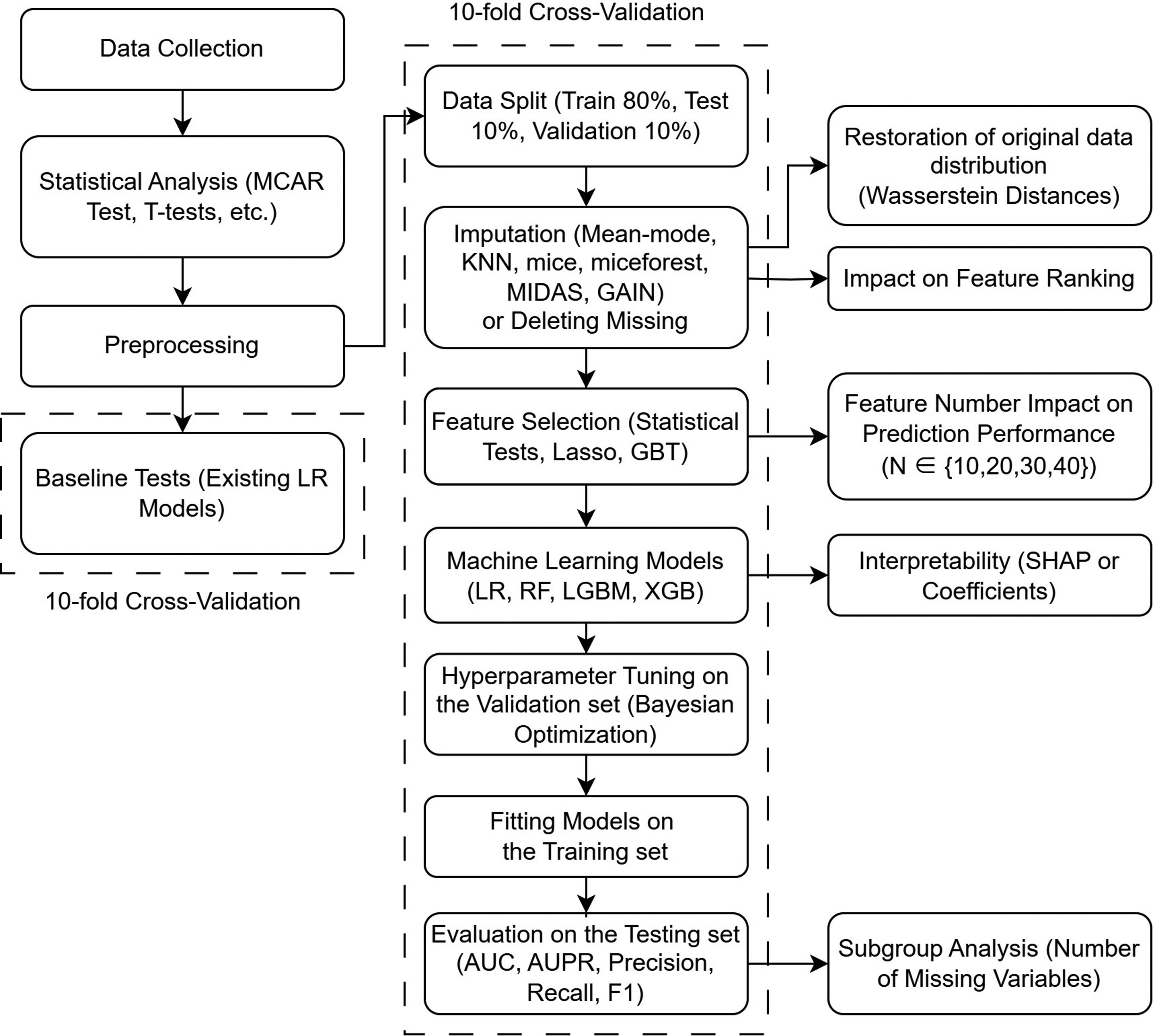
Workflow of model development and evaluation.

Data collection and preprocessing

This retrospective study collected data from pregnant women who delivered at Peking Union Medical College Hospital (PUMCH) in Beijing, China, from July 1, 2020, to June 30, 2022. A total of 5409 women with singleton pregnancies, aged 18 to 50 years, were identified. Our inclusion criteria included: (a) registration for perinatal care at PUMCH, (b) single pregnancy, (c) early pregnancy (at 0–12 weeks gestation). Our exclusion criteria were: (a) a history of type 1 or type 2 diabetes (N = 128), (b) failure to participate in 75 g OGTT screening within 24–28 weeks or loss of 75 g OGTT data (N = 215). The final dataset consisted of 5066 individual cases. The gold standard for GDM diagnosis was based on the International Association of Diabetes and Pregnancy Study Groups (IADPSG) guidelines.⁷

As we used anonymized and deidentified data and did not constitute human research, the need for written informed consent was waived by the Ethics Review Board of the PUMCH due to the retrospective nature of the study. This study was approved by the Ethics Review Board of Peking Union Medical College Hospital, Chinese Academy of Medical Sciences (I-22PJ122). All procedures were performed by the Declaration of Helsinki.

The predictor variables comprised clinical and demographic parameters obtained from maternal EHRs: (a) basic characteristics, including maternal age, parity, and gravidity, recorded in pregnancy files; (b) physical measurements, including height and weight before pregnancy; (c) maternal medical history, including smoking, drinking, history of abnormal pregnancy, abortion, GDM, macrosomia, and polycystic ovary syndrome; and (d) family history of hypertension and diabetes. Laboratory tests included: (a) liver function tests, (b) renal function tests, (c) fasting blood glucose levels, (d) lipid metabolism tests, (e) thyroid function tests, (f) complete blood count, and (g) nutritional tests for iron and iodine.

The dataset was preprocessed to improve the overall performance. First, new categorical variables were introduced into our dataset. Categorical variables were created to indicate gravidity (history of pregnancy), parity (history of childbirth), advanced maternal age (35 years old and over), and pre-diabetes (fasting plasma glucose ≥ 5.1 mmol/L).⁷ Body mass index (BMI) was categorized based on Chinese obesity standards³³ into four groups (0, 1, 2, 3). Then, non-continuous and non-binary variables were one-hot encoded to improve compatibility with imputation models like MIDAS. Continuous variables were standardized for better imputation and data comparability. To avoid excessive bias, we deleted 7 features with a missing rate greater than 80%, including HbA1C, TSAT, TIBC, Fe, GA%, Hcy, and SF. After preprocessing, the resulting dataset comprised 93 features (maximum missing data rate: 75.25%) and 926 complete cases (no missing data), hereafter referred to as the “no-missing dataset.”

Statistical analysis

Little's missing completely at random (MCAR) test is used to determine whether the missing data are missing completely at random by IBM SPSS Statistics for Windows, version 25.0 (Armonk, NY: IBM Corp). The Python package SciPy (https://scipy.org/) running on Python 3.9 was employed for the following statistical analysis. Normality tests were conducted based on the D’Agostino and Pearson test. For continuous variables with a normal distribution, the t-test was used for comparison. For non-normally distributed continuous variables, the Mann–Whitney U test was applied. Categorical data were analyzed using the χ² test. The Friedman test was used to examine whether different imputation methods show significant differences in GDM prediction performance.

Workflow

Before developing our own models, we tested two available logistic regression models proposed in previous literature as baselines. They were both conducted on Chinese people, consistent with our sample.^18,34 The baseline tests serve two purposes: (a) to highlight differences in data distribution across studies, which represents a primary limitation in the generalization of medical AI applications,³⁵ and (b) to demonstrate the impact of missing data on predictive modeling. We excluded cases with any missing variables for the two models, leading to a significant reduction in the size of both the training and test sets. We trained the two models separately using variables from both models on our data. For these two models, we used 10-fold cross-validation the same as with machine learning models. The AUCs of the two models are reported in the “Result” section.

To prevent any potential data leakage, we strictly segregated the training and test sets before the imputation phase.³⁶ The original data was randomly divided into a training set and a test set at a 90:10 ratio. All imputation models were fitted on the training set without the target variable “GDM” and subsequently used to impute values in the test set. Then, 1/9 of the training set was randomly sampled as the validation set for parameter tuning. This resulted in a final split of 80% for training, 10% for testing, and 10% for validation. To ensure a fair evaluation of the imputation model's generalizability, we performed a 10-fold cross-validation outside the entire imputation-prediction process.³⁷ This approach effectively mitigates potential biases introduced by repeated imputation procedures. Unless otherwise stated, all evaluation metrics are averaged based on 10-fold cross-validation.

Imputation methods

The imputation methods assessed in this study comprised mean-mode imputation, KNN imputation, MICE, MIDAS, and GAIN. Thus, traditional methods, advanced methods and emerging deep learning methods are taken into account. Supplementary Table S1 provides the hyperparameter settings of imputation methods. For multiple imputation methods such as MICE, MIDAS, and GAIN, we generated five imputed datasets and develop a predictive model on each of them in one cross-validation loop. The final prediction for each individual was obtained by averaging the predicted probabilities across the models, in order to account for the uncertainty introduced by multiple imputation in accordance with Rubin's rules for combining estimates.³⁸

Mean-mode imputation uses the mean to fill in missing values for numerical features and the most frequently occurring category (mode) for categorical features. KNN imputation is based on the values of KNN in the observed data. Discrete variables are rounded. The Python package sklearn (http://scikit-learn.org) was used for Mean-mode and KNN.

The MICE method is one of the most commonly used methods to handle missing data.^39,40 In this study, we chose two robust models, classification and regression tree (CART) and LGBM, to be used within MICE. We used the R package mice (https://CRAN.R-project.org/package=mice) and the Python package miceforest (https://pypi.org/project/miceforest/) to implement the two kinds of MICE. In this study, the two methods are referred to as “mice” and “miceforest,” respectively.

Multiple imputation with denoising autoencoders (MIDAS) is a fast multiple imputation method based on deep learning. MIDAS employs a class of unsupervised neural networks known as denoising autoencoders. Compared with conditional imputation, MIDAS provides higher accuracy while completing imputation much more quickly. We used the Python package MIDASpy for a rapid deployment.⁴¹

Yoon proposed generative adversarial imputation nets (GAIN), which surpassed multivariate imputation methods such as missforest in multiple datasets.⁴² Considering the potential of adversarial generative networks in imputation, we chose GAIN as another deep learning method. The Python package hyperimpute was used for GAIN.⁴³

Feature selection

Feature selection was conducted after imputation. We integrated three different methods to pick the most relevant features for prediction. The first method was a statistical approach. We employed t-tests, the Mann–Whitney U test, and the χ² test to calculate p-values, which served as criteria for selecting significant features. Second, we used lasso regression to avoid collinearity problems, ranking feature importance based on the absolute values of the coefficients. Third, we used a machine learning method, gradient boosting tree (GBT), to evaluate feature importance. Feature selection was based on the average ranking of feature importance from the three methods. To reduce the dimensionality of the data after preprocessing, we selected the top N features, using values of N from the set {10, 20, 30, 40}. Adhering to the recommended minimum of 20 events per variable (EPV) for reliable model development,⁴⁴ our whole dataset (N = 5066) is sufficient to support the development of models comprising up to 40 features.

Machine learning models

We evaluated the performance of four widely used machine learning models after handling the missingness—logistic regression (LR), random forest (RF), LightGBM (LGBM), and XGBoost (XGB).^45,46 For LR and RF, we utilized implementations from the scikit-learn library. LGBM was implemented using the LightGBM package (https://pypi.org/project/lightgbm/), while the XGBoost package (https://pypi.org/project/xgboost/) was used for the deployment of XGB. Hyperparameter tuning for all models was conducted using Bayesian optimization. Detailed hyperparameter optimization ranges are provided in Supplementary Table S2.

Evaluation

Various metrics were employed to assess imputation-based predictive model performance. We reported the AUC, the area under the precision-recall curve (AUPR), precision (P), recall (R), and F1-score (F1) for each experimental combination. All metrics were presented as cross-validated averages. The Youden index was used to determine the optimal cutoff values. We also repeated the experiments with the dominant predictor, “history of GDM,” excluded. This was done to prevent this complete feature from confounding the evaluation of imputation's impact on other variables and to enhance the generalizability of our findings.

Metrics commonly used to evaluate data reconstruction, such as mean absolute error (MAE) and mean squared error (MSE), were not applicable in this study due to the unknown true values in the original data. Given the discrepancy in case numbers between the fully complete subsets and the original dataset (926 vs. 5066), a fair evaluation of imputation methods might not be achievable using only the fully complete subsets. Therefore, we calculated the Wasserstein distances (WS distances) between the original and imputed data to evaluate the ability of imputation methods to recover the original distribution, that is, their fit to the data distribution. For methods supporting multiple imputations, distances were computed for each imputation replicate and pooled using arithmetic means.³⁸ WS distance allows comparison between lists of different lengths. A smaller WS distance indicates an easier transition between the two distributions.⁴⁷

We additionally conducted a subgroup analysis on the number of missing variables for each case in the test set to demonstrate the applicability of the imputation methods. The number of missing features per case ranged from 0 to 52, with a median of 6. Accordingly, we stratified the data into four subsets: [0, 3), [3, 6), [6, 9), and [9, 53), where each interval includes the lower bound but excludes the upper bound. For example, [0, 3) includes cases with 0, 1, or 2 missing features. The F1-score, recall, and precision were calculated using the cutoff values obtained from the whole test sets.

Finally, we tested how predictive performance changed with feature rankings provided by different imputation methods, while simultaneously trying to find a minimum effective subset of features. Narrowing down to a smaller subset of features benefits the decision-making process for clinicians, enhancing practicality and efficiency. The optimal prediction model in previous experiments was tested on the imputed dataset with the smallest WS distance, incrementally adding variables according to the rankings established in the feature selection step. We conducted 10-fold cross-validation, and for each fold, LR with fixed hyperparameters was performed on five multiple imputed datasets during the process. In the interest of interpretability, we reported the model coefficients, as the best prediction model was a LR model.

Result

Participants

We identified 1094 cases of GDM within our dataset, resulting in an overall incidence rate of 21.59%. When we considered only the subset with complete data (N = 926), the GDM incidence was 22.89%. Table 1 presents descriptive statistics and missing rates for variables that demonstrated statistical significance (p < 0.05), including 27 variables. The raw data had a maximum missing rate of 95.5% and an average missing rate of 17.92%. There were 13 variables with missing rates greater than 50%. Only 63 cases were complete. The p-value of Little's MCAR test was less than 0.001, which rejected the null hypothesis that the dataset was MCAR. The missing patterns of 10 variables (A-TPO, A-Tg, FT3, FT4, HDL-C, HbA1C, LDL-C, TC, TG, TSH) correlated with the value of GDM (1 representing diagnosed with GDM, 0 representing normal). Descriptive statistics and abbreviations for all 55 variables are shown in Table S3 of the supplementary material.

Table 1.

Variables with statistical significance (p < 0.05).

Variables	Non-GDM (mean ± std)	GDM (mean ± std)	p-Value	Total missing rate	Non-GDM missing rate	GDM missing rate
Age (year)	32.11 ± 3.79	33.60 ± 3.87	<0.001	0.00%	0.00%	0.00%
PAB	240.91 ± 30.77	252.62 ± 32.96	<0.001	2.39%	2.40%	2.33%
BMI	21.48 ± 2.80	22.37 ± 3.14	<0.001	0.00%	0.00%	0.00%
GGT	16.25 ± 9.19	19.44 ± 14.62	<0.001	3.24%	3.25%	3.17%
Family history of diabetes			<0.001	0.00%	0.00%	0.00%
No	3284	765
Yes	711	306
FPG	4.64 ± 0.44	4.77 ± 0.54	<0.001	1.80%	1.83%	1.68%
WBC	8.17 ± 2.06	8.68 ± 2.15	<0.001	1.03%	1.03%	1.03%
PLT	247.76 ± 51.78	260.24 ± 57.73	<0.001	1.05%	1.05%	1.03%
TG	0.92 ± 0.45	1.13 ± 0.67	<0.001	66.82%	67.51%	64.24%
Weight (kg)	57.94 ± 8.17	59.75 ± 8.82	<0.001	0.00%	0.00%	0.00%
HGB	129.22 ± 9.06	131.01 ± 8.91	<0.001	1.05%	1.08%	0.93%
History of GDM			<0.001	0.00%	0.00%	0.00%
No	3986	1055
Yes	9	16
ALT	17.06 ± 14.64	19.28 ± 17.88	<0.001	1.72%	1.70%	1.77%
ALP	48.21 ± 11.05	50.37 ± 12.35	<0.001	3.22%	3.28%	2.99%
LDL-C	2.21 ± 0.57	2.40 ± 0.71	<0.001	67.02%	67.73%	64.33%
Height (cm)	164.22 ± 5.11	163.42 ± 5.18	<0.001	0.00%	0.00%	0.00%
TC	4.19 ± 0.69	4.39 ± 0.85	<0.001	67.59%	68.14%	65.55%
History of abnormal pregnancy			<0.001	0.00%	0.00%	0.00%
No	2780	681
Yes	1215	390
Family history of hypertension			<0.001	0.00%	0.00%	0.00%
No	2754	674
Yes	1241	397
NEUT%	69.93 ± 6.65	70.76 ± 6.41	<0.001	1.05%	1.05%	1.03%
HbA1C	5.06 ± 0.29	5.22 ± 0.46	0.001	95.54%	95.84%	94.40%
TIBC	330.38 ± 53.77	347.63 ± 61.81	0.008	87.43%	87.16%	88.42%
PCOS			0.020	0.00%	0.00%	0.00%
No	2787	707
Yes	1208	364
HDL-C	1.52 ± 0.29	1.48 ± 0.29	0.034	67.09%	67.78%	64.52%
uGLU	0.06 ± 0.36	0.09 ± 0.47	0.037	0.06%	0.05%	0.09%
Gravidity	1.77 ± 1.04	1.84 ± 1.08	0.046	0.00%	0.00%	0.00%
History of miscarriage			0.048	0.00%	0.00%	0.00%
No	2558	650
Yes	1437	421

Note: PAB, prealbumin (mg/L); BMI, body mass index (kg/m²); GGT, gamma-glutamyl transferase (U/L); FPG, fasting plasma glucose (mmol/L); WBC, white blood cell count (10⁹/L); PLT, platelet count (10⁹/L); TG, triglycerides (mmol/L); HGB, hemoglobin (g/L); ALT, alanine aminotransferase (U/L); ALP, alkaline phosphatase (U/L); LDL-C, low-density lipoprotein cholesterol (mmol/L); TC, total cholesterol (mmol/L); NEUT%, neutrophil percentage (%); HbA1C, hemoglobin A1C (%); TIBC, total iron-binding capacity (μg/dL); uBLD, urine occult blood (an ordinal variable with an integer value from 0 to 4 depending on the concentration of urine occult blood); HDL-C, high-density lipoprotein cholesterol (mmol/L); uGLU, urine glucose (an ordinal variable ranging from 0 to 5 based on the concentration of glucose in the urine).

Baseline models

Two available prediction models were tested as the baselines on our dataset. Duo et al. trained LR models including “age,” “BMI,” “family history of diabetes,” “FPG,” “ALT/AST,” and “TG/HDL-C” (AUC = 0.825, N = 1289).¹⁸ Guo et al. used fewer variables to construct the LR model, only using “age,” “BMI,” “family history of diabetes,” and “FPG” (AUC = 0.69, N = 6572).³⁴ Our data yielded worse results for both models (AUC = 0.6350, N = 1647 for Duo's and AUC = 0.6497, N = 4975 for Guo's). The larger dataset used by Guo et al. may partially explain the discrepancy with published results. The above results indicate that missing data seriously affects the performance of prediction models in clinical practice.

Imputation-based machine learning prediction

Table 2 provides the AUCs resulting from combinations of various imputation methods and prediction models. Based on the average AUCs across all models, miceforest imputation performed the best when feature number was set to 20, 30, and 40. The mean-mode method was better than the others when the number of features was 20, while mice imputation exhibited superior performance in all other feature number settings. The Friedman test showed that the differences among imputation methods were approaching significance (p = 0.3539).

Table 2.

GDM prediction AUC by imputation methods and machine learning models.

Feature number	Imputation	LGBM	LR	RF	XGB	Average
10	GAIN	0.6362	0.6756	0.6431	0.6101	0.6412
	KNN	0.6329	0.6747	0.6410	0.6099	0.6396
	mice	0.6455	0.6812	0.6481	0.6204	0.6488
	miceforest	0.6419	0.6785	0.6470	0.6232	0.6477
	MIDAS	0.6457	0.6787	0.6496	0.6285	0.6506
	Mean-mode	0.6302	0.6777	0.6374	0.6050	0.6376
	No Missing	0.6095	0.6520	0.6334	0.5913	0.6216
20	GAIN	0.6510	0.6872	0.6562	0.6337	0.6570
	KNN	0.6348	0.6870	0.6480	0.6075	0.6443
	mice	0.6507	0.6890	0.6577	0.6359	0.6583
	miceforest	0.6588	0.6870	0.6586	0.6355	0.6600
	MIDAS	0.6489	0.6862	0.6548	0.6323	0.6556
	Mean-mode	0.6418	0.6893	0.6546	0.6054	0.6478
	No Missing	0.5991	0.6414	0.6309	0.6260	0.6244
30	GAIN	0.6544	0.6863	0.6484	0.6248	0.6535
	KNN	0.6377	0.6867	0.6474	0.6036	0.6439
	mice	0.6541	0.6899	0.6512	0.6395	0.6587
	miceforest	0.6579	0.6886	0.6556	0.6442	0.6616
	MIDAS	0.6537	0.6854	0.6551	0.6293	0.6559
	Mean-mode	0.6413	0.6875	0.6392	0.6103	0.6446
	No Missing	0.6069	0.6336	0.6668	0.6369	0.6361
40	GAIN	0.6442	0.6827	0.6461	0.6247	0.6494
	KNN	0.6387	0.6830	0.6439	0.6006	0.6415
	mice	0.6533	0.6873	0.6551	0.6361	0.6580
	miceforest	0.6578	0.6829	0.6525	0.6417	0.6587
	MIDAS	0.6530	0.6814	0.6528	0.6373	0.6561
	Mean-mode	0.6345	0.6849	0.6374	0.6116	0.6421
	No Missing	0.6133	0.6353	0.6604	0.6188	0.6320

At the level of prediction models, LR consistently exhibited its advantages, as observed from the color fill in Table 2. When using the top 30 features, the LR with mice imputation reached the highest AUC of 0.6899, compared to 0.6336 for the LR model without imputation. The 20-feature LR with mean-mode obtained the second best AUC (0.6893) among all combinations. It is worth noting that the AUC of the LR without imputation declined with increasing numbers of features, even falling below the AUC of a baseline model at 20 features. This could indicate overfitting due to the small dataset size. While imputation significantly improved LR and LGBM, RF and XGB did not benefit much. The observed advantage in mice persisted even after excluding the dominant risk factor, “history of GDM” (see Supplementary Table S4),⁴⁸ indicating that imputation, rather than the non-missing dominant variable, primarily drove the improvement.

Given the optimal performance of the 30-feature group, subsequent evaluation concentrated on its remaining metrics (Supplementary Table S5). Analysis of performance metrics for the LR model with 30 features revealed that while imputation enhanced the average AUC, the best AUPR was achieved by LR trained on the no-missing dataset. RF trained on the no-missing dataset showed the best recall (0.7403) and F1-score (0.4577) among all the combinations. The RF model with GAIN imputation demonstrated superior performance in terms of specificity and precision, achieving values of 0.7629 and 0.3743, respectively. GAIN imputation yielded the best average specificity.

Subgroup analysis

The 30-feature group performed the best, so the subgroup analysis focused on its results. The corresponding average number of cases in each subset across the cross-validation folds was 133.9, 33, 339.7, and 42.1, respectively.

Figure 2 illustrates the changes in F1-score, recall, and precision across these subsets. On the whole, there was a loss of performance as the number of missing features increased. Different imputation methods exhibited similar patterns of fluctuation. However, the miceforest methods produced a distinctly curved upward trajectory for LR's recall and F1-scores. Furthermore, the miceforest consistently produced stable F1-scores. XGB exhibited notable sensitivity to the imputation methods and the number of missing variables. All methods had a precision peak in [3, 6) groups, likely because of the small sample sizes.

Figure 2.

Influence of imputation strategy and missing value count on classification metrics.

Restoration of original data distribution

The WS distance was generated by comparing different imputed datasets to the original dataset. A single comparison for each variable generated a WS distance. Figure 3 shows that the 25th percentile and median of WS distances across all imputation methods were nearly identical. However, the 75th percentile and upper whisker differed substantially among the methods. Mice performed the best in terms of the interquartile range (IQR), suggesting that mice was more effective at estimating variables with high missing rates, as the WS distance is correlated with missingness. GAIN, KNN, and MIDAS performed worse than miceforest, while the mean-mode method performed the worst.

Figure 3.

Wasserstein distance between original and imputed data distributions. Outliers are not shown.

In summary, the MICE-based methods achieved the best overall performance in approximating the distribution of the original dataset.

Features ranking and interpretability

LR outperformed all models and mice imputation demonstrated the best overall performance. We conducted tests on mice-imputed datasets to observe how the performance of this combination changed as the number of features varied. The feature importance rankings obtained from the feature selection step are shown in Supplementary Table S6. All rankings generated by imputation were similar, which means the feature importance rankings were not sensitive to the imputation methods. Only the ranking from the no-missing dataset differed significantly from the others, and led to worse downstream performance, as shown in Figure 4. We re-evaluated two baseline models using the same mice-imputed datasets. The LR model proposed by Duo et al.¹⁸ exhibited an AUC of 0.6656 on the mice-imputed dataset and the model developed by Guo et al.³⁴ achieved an AUC of 0.6582. As the number of features increased, the average AUC slightly declined. Fewer features effectively predict early GDM. Figure 4 shows that the top 18 features identified by the mean-mode method were sufficient to bring the LR model close to its maximum performance. However, the AUC of the 18-feature LR model decreased to 0.6647 when cases with missing data were removed (N = 1315), highlighting the data enhancement capabilities of imputation. The regression coefficients based on mice-imputed datasets were aggregated and visualized as a boxplot in Figure 5. Since the dataset is standardized, these coefficients can be considered as the relative importance of features.

Figure 4.

Average AUC of LR on the mice-imputed dataset using different feature rankings.

Figure 5.

Box plot of coefficients from 10-fold cross-validation on the mice-imputed datasets. PAB, prealbumin; BMI, body mass index; GGT, gamma-glutamyl transferase; LDL-C, low-density lipoprotein cholesterol; FPG, fasting plasma glucose; WBC, white blood cell count; HGB, hemoglobin; NEUT%, neutrophil percentage; PLT, platelet count; TG, triglycerides; TC, total cholesterol; Cr, creatinine; uGLU_0.0, 1 represents no urinary glucose detected. 0 represents urinary glucose is detected.

Discussion

By jointly analyzing imputation approaches and downstream classifiers, this study assessed their combined influence on early GDM prediction performance based on incomplete EHR datasets. Mice achieved the highest AUC of 0.6899 and yielded the best data distribution restoration, consistent with previous findings.^49,50 The LR model trained on mice-imputed data with an optimized feature set achieved the best performance among all experiments, with an AUC of 0.6901. Mice may be the preferred default method when its computational cost and the inherent uncertainty of multiple imputation are not primary concerns. Surprisingly, the mean-mode imputation with LR achieved the second best AUC (0.6893) and provided an effective feature subset, though mean-mode imputation caused greatest distributional bias. When the classifier was LR, the mean-mode method outperformed MICE-based methods when the top-20 features were using. This may result from that the mean-mode imputation is particularly suited for skewed distributions with high missing rates, where it is challenging for imputation algorithms to learn the data patterns.³⁰ The simple imputation method may also play a regularizing role, reducing variance by shrinking imputed values toward the mean, thereby preventing the model from overfitting.⁴⁹ The mean-mode method is generally not recommended because it leads to biased estimates of statistics.⁵¹ Nevertheless, given its superior performance in downstream predictive tasks, the mean-mode imputation method may be considered acceptable for training and applying GDM prediction models. KNN is another competitive simple imputation method. When combined with LR, it yielded a slightly lower AUC than the mean-mode method but performed best in terms of specificity and precision, and provided a better fit to the data. Although GAIN imputation significantly improved specificity, its AUC performance was suboptimal. Generation-based imputation methods did not outperform traditional methods, potentially attributed to the relatively low dimensionality of our dataset compared to studies where generation models showed superior results.^31,42,52 The models trained on the no-missing dataset demonstrated the highest average AUPR. The RF model trained on the no-missing dataset exhibited superior recall and F1-score compared to all other imputation-prediction method combinations. In practical applications, a complementary approach that combines the model trained with imputed data and the one trained without missing data can be considered to enhance overall predictive capability.

The classification method primarily accounted for the differences in predictive performance. Complex machine learning models, such as XGB, appeared more sensitive to noise introduced by imputation, leading to worse performance compared to traditional models like logistic regression with L2 regularization. XGB exhibited poorer performance with imputation methods that had larger Wasserstein distances (i.e. mean-mode imputation). These findings suggest that for datasets with high missingness, the choice of classifier should be made with caution.

The subgroup analysis demonstrates that LR with mice is robust to variations in the number of missing variables. In addition to mice's strong fitting performance, this robustness may be attributed to the feature selection stage applied to the imputed dataset, which balances the level of missingness and feature importance, thereby mitigating the impact of missing data in individual features. This finding supports the use of mice to enhance predictive models in clinical environments, where the extent of missing data can vary substantially across patient records. Integrating imputation into hospital risk prediction workflows holds promise for improving patient equity, given the widespread prevalence of missing data in clinical settings.

The effect of the number of features was analyzed based on mice imputation, identifying 18 key features for GDM prediction in the Chinese population. These features include age, personal and family disease history, physical examination findings, complete blood count, liver and kidney function parameters, and lipid-related biomarkers. Except for the last one, all features can be obtained from routine medical checkups, indicating the high practical applicability of the 18-feature model. The underperformance of the two external models may be attributable to earlier gestational age and regional differences. However, our results suggest that these gaps can be addressed using a few more features. Our results indicate that including more features can lead to overfitting when training on small datasets, but imputation can help mitigate this issue. It is recommended to consider simultaneously hematology, lipid profiles,^53,54 liver function, and kidney function⁵⁵ when predicting the risk of GDM. This combination of factors provides models with good discriminatory ability, even in the absence of GDM history. Imputation facilitates the inclusion of a greater number of informative features in prediction models with large sample sizes, further underscoring its necessity in clinical predictive modeling.

Notably, significant differences were observed in the feature importances derived from the imputed dataset compared to the dataset without missing values. Consequently, the feature ranking obtained from the dataset without missing values could not maximize downstream model performance when applied to the imputed dataset. This highlights the impact of the bias introduced by missing data and underscores the importance of conducting sensitivity analyses on prediction models to ensure reliable results.¹⁴

Our primary contribution lies in demonstrating the effectiveness and necessity of integrating imputation into EHR-based GDM prediction through extensive analyses. We also provide practical recommendations on optimizing the synergy between imputation methods and predictive modeling. However, this study has some limitations. Firstly, as a single-center retrospective study, it was constrained by limited sample size and diversity, and we were unable to perform external validation. Secondly, while we conducted various experiments, the highest AUC achieved is 0.6901, below the commonly accepted threshold of 0.7 for moderate diagnostic ability.⁵⁶ Achieving significantly higher discrimination might require a larger sample size or additional clinical, genetic, or microbiomic features than were available in this study.^27,57,58

Building upon these findings, several directions warrant future investigation to advance robust and equitable GDM prediction systems. Future research should assess the capability of more advanced imputation methods, such as pre-trained models,⁵⁹ in enhancing prediction. Next, future work should focus on building integrated predictive frameworks that combine conventional clinical features with emerging biomarkers.¹³ Subsequently, external validation should be conducted across multiple institutions and populations to evaluate the generalizability and fairness of imputation-based predictive models. Finally, the practical feasibility of deploying imputation-integrated prediction workflows into clinical decision support systems requires exploration, including aspects such as computation time, clinician trust, and long-term maintenance.⁶⁰

Conclusion

This study demonstrates that effective imputation of missing data significantly enhances early prediction of GDM and improves patient equity. During imputation-based machine learning model development, careful model selection is required to prevent degradation, such as the decline in XGB performance observed in this study. In contrast, imputation consistently improved the AUC of LR for GDM prediction. MICE-based methods remain a reliable default when computational resources are not a constraint. Mean-mode imputation, despite its statistical simplicity, shows strong predictive performance when paired with LR. The identification of 18 key features highlights the importance of routine medical checkups in early GDM prediction. Imputation enhances the model's capacity to incorporate relevant features, improving the predictive performance and robustness of the risk assessment.

In summary, these findings provide empirical guidance for addressing missing data in GDM model development. Furthermore, they inform future research into imputation methodologies and demonstrate the potential of integrating imputation into clinical prediction models.

Supplemental Material

sj-docx-1-dhj-10.1177_20552076251352436 - Supplemental material for Enhancing early gestational diabetes mellitus prediction with imputation-based machine learning framework: A comparative study on real-world clinical records

Supplemental material, sj-docx-1-dhj-10.1177_20552076251352436 for Enhancing early gestational diabetes mellitus prediction with imputation-based machine learning framework: A comparative study on real-world clinical records by Leyao Ma, Lin Yang, Yaxin Wang, Jie Hao, Yini Li, Liangkun Ma, Ziyang Wang, Ye Li, Suhan Zhang, Mingyue Hu, Jiao Li and Yin Sun in DIGITAL HEALTH

Supplemental Material

sj-pdf-2-dhj-10.1177_20552076251352436 - Supplemental material for Enhancing early gestational diabetes mellitus prediction with imputation-based machine learning framework: A comparative study on real-world clinical records

Supplemental material, sj-pdf-2-dhj-10.1177_20552076251352436 for Enhancing early gestational diabetes mellitus prediction with imputation-based machine learning framework: A comparative study on real-world clinical records by Leyao Ma, Lin Yang, Yaxin Wang, Jie Hao, Yini Li, Liangkun Ma, Ziyang Wang, Ye Li, Suhan Zhang, Mingyue Hu, Jiao Li and Yin Sun in DIGITAL HEALTH

Footnotes

Acknowledgments

The authors would like to thank the participants of this study, as well as the clinicians and information staff at Peking Union Medical College Hospital for the data collection in this study.

ORCID iDs

Leyao Ma

Lin Yang

Yaxin Wang

Jie Hao

Yini Li

Liangkun Ma

Ziyang Wang

Ye Li

Suhan Zhang

Mingyue Hu

Jiao Li

Yin Sun

Ethical considerations

This study was approved by the Ethics Review Board of PUMCH, Chinese Academy of Medical Sciences (JS-2763).

Consent to participate

Author contributions

Conceptualization was done by LKM, YS, and JL; methodology was accomplished by LY, JH, YXW; formal analysis and data curation were done by LYM, YNL, ZYW, and SHZ; writing—original draft preparation by LYM, MYH and LY; writing—review and editing by LY, JH and YXW; supervision by LKM, YS and JL.

Funding

The authors disclosed receipt of the following financial support for the research, authorship, and/or publication of this article: This study was supported by the China Medical Board (CMB-OC, Q629500), Science and Technology Project of Beijing (Z231100004623010), the Chinese Academy of Medical Sciences (CAMS) Innovation Fund for Medical Sciences (CIFMS; grant 2021-I2M-1-056, and 2021-I2M-1-023).

Data availability statement

The datasets generated and analyzed during the current study are available from the corresponding author on reasonable request.

Declaration of conflicting interests

The authors declared no potential conflicts of interest with respect to the research, authorship, and/or publication of this article.

Guarantor

Dr Jiao Li and Dr Ying Sun.

Supplemental material

Supplemental material for this article is available online.

Peer review

None.

References

Sweeting

Wong

Murphy

, et al. A clinical update on gestational diabetes mellitus. Endocr Rev 2022; 43: 763–793.

McIntyre

Catalano

Zhang

, et al. Gestational diabetes mellitus. Nat Rev Dis Primer 2019; 5: 1–19.

Wang

Chivese

, et al. IDF diabetes atlas: estimation of global and regional gestational diabetes mellitus prevalence for 2021 by International Association of Diabetes in Pregnancy Study group’s criteria. Diabetes Res Clin Pract 2022; 183: 109050.

Jiang

Tang

Magee

, et al. A global view of hypertensive disorders and diabetes mellitus during pregnancy. Nat Rev Endocrinol 2022; 18: 760–775.

Modzelewski

Stefanowicz-Rutkowska

Matuszewski

, et al. Gestational diabetes mellitus-recent literature review. J Clin Med 2022; 11: 5736.

Yan

Y-S

Feng

D-Q

, et al. Long-term outcomes and potential mechanisms of offspring exposed to intrauterine hyperglycemia. Front Nutr 2023; 10: 1067282.

International Association of Diabetes and Pregnancy Study Groups Consensus Panel. International Association of Diabetes and Pregnancy Study groups recommendations on the diagnosis and classification of hyperglycemia in pregnancy. Diabetes Care 2010; 33: 676–682.

Ryan

Haddow

Ramaesh

, et al. Early screening and treatment of gestational diabetes in high-risk women improves maternal and neonatal outcomes: a retrospective clinical audit. Diabetes Res Clin Pract 2018; 144: 294–301.

Simmons

Immanuel

Hague

, et al. Treatment of gestational diabetes mellitus diagnosed early in pregnancy. N Engl J Med 2023; 388: 2132–2144.

10.

Galdikaitė

Simanauskaitė

Ramonienė

, et al. The effect of timing and methods for the diagnosis of gestational diabetes mellitus on obstetric complications. Med Kaunas Lith 2023; 59: 854.

11.

Hillier

Pedula

Ogasawara

, et al. Impact of earlier gestational diabetes screening for pregnant people with obesity on maternal and perinatal outcomes. J Perinat Med 2022; 50: 1036–1044.

12.

Saravanan

Deepa

Ahmed

, et al. Early pregnancy HbA1c as the first screening test for gestational diabetes: results from three prospective cohorts. Lancet Diabetes Endocrinol 2024; 12: 535–544.

13.

Parkhi

Sampathkumar

Weldeselassie

, et al. Systematic review of risk score prediction models using maternal characteristics with and without biomarkers for the prediction of GDM. medRxiv. 2023; 2023.10.23.23297401.

14.

Little

D’Agostino

Cohen

, et al. The prevention and treatment of missing data in clinical trials. N Engl J Med 2012; 367: 1355–1360.

15.

Chang

H-H

Hsu

T-C

Hsieh

Y-H

, et al. Meta-EHR: a meta-learning approach for electronic health records with a high imbalanced ratio and missing rate. In: 2023 45th Annual International Conference of the IEEE Engineering in Medicine & Biology Society (EMBC) , pp.1–4.

16.

Zhang

Yang

Han

, et al. Machine learning prediction models for gestational diabetes mellitus: meta-analysis. J Med Internet Res 2022; 24: e26634.

17.

Y-T

Zhang

C-J

Mol

, et al. Early prediction of gestational diabetes mellitus in the Chinese population via advanced machine learning. J Clin Endocrinol Metab 2021; 106: e1191–e1205.

18.

Duo

Song

Qiao

, et al. A simplified screening model to predict the risk of gestational diabetes mellitus in pregnant Chinese women. Diabetes Ther Res Treat Educ Diabetes Relat Disord 2023; 14: 2143–2157.

19.

Cubillos

Monckeberg

Plaza

, et al. Development of machine learning models to predict gestational diabetes risk in the first half of pregnancy. BMC Pregnancy Childbirth 2023; 23: 469.

20.

Ayilara

Zhang

Sajobi

, et al. Impact of missing data on bias and precision when estimating change in patient-reported outcomes from a clinical registry. Health Qual Life Outcomes 2019; 17: 106.

21.

Getzen

Ungar

Mowery

, et al. Mining for equitable health: assessing the impact of missing data in electronic health records. J Biomed Inform 2023; 139: 104269.

22.

Zhang

Yang

Han

, et al. Machine learning prediction models for gestational diabetes mellitus: meta-analysis. J Med Internet Res 2022; 24: e26634.

23.

Islam

Mustafina

Mahmud

, et al. Machine learning to predict pregnancy outcomes: a systematic review, synthesizing framework and future research agenda. BMC Pregnancy Childbirth 2022; 22: 348.

24.

Gabbay-Benziv

Doyle

Blitzer

, et al. First trimester prediction of maternal glycemic status. J Perinat Med 2015; 43: 283–289.

25.

Sweeting

Wong

Appelblom

, et al. A novel early pregnancy risk prediction model for gestational diabetes mellitus. Fetal Diagn Ther 2019; 45: 76–84.

26.

Ruiter

Kwee

Naaktgeboren

, et al. External validation of prognostic models to predict risk of gestational diabetes mellitus in one Dutch cohort: prospective multicentre cohort study. Br Med J 2016; 354: i4338.

27.

Zaky

Fthenou

Srour

, et al. Machine learning based model for the early detection of gestational diabetes mellitus. BMC Med Inform Decis Mak 2025; 25: 130.

28.

Yan

Chaudhary

, et al. Imputation of missing values for electronic health record laboratory data. Npj Digit Med 2021; 4: 1–14.

29.

Germaine

O’Higgins

Egan

, et al. Evaluation of machine learning models for early prediction of gestational diabetes using retrospective electronic health records from current and previous pregnancies. medRxiv 2025; 2025.05.12.25327431.

30.

Jäger

Allhorn

Bießmann

. A benchmark for data imputation methods. Front Big Data 2021; 4: 693674. https://www.frontiersin.org/articles/10.3389/fdata.2021.693674 .

31.

Beaulieu-Jones

Moore

. Missing data imputation in the electronic health record using deeply learned autoencoders. Pac Symp Biocomput Pac Symp Biocomput 2017; 22: 207–218.

32.

Alabadla

Sidi

Ishak

, et al. Systematic review of using machine learning in imputing missing values. IEEE Access 2022; 10: 44483–44502.

33.

Chinese Nutrition Society Obesity Prevention and Control Section, Chinese Nutrition Society Clinical Nutrition Section, Chinese Preventive Medicine Association Behavioral Health Section , et al. Expert consensus on obesity prevention and treatment in China. Chin J Epidemiol 2022; 43: 609–626.

34.

Guo

Yang

Zhang

, et al. Nomogram for prediction of gestational diabetes mellitus in urban, Chinese, pregnant women. BMC Pregnancy Childbirth 2020; 20: 43.

35.

Yang

Zhang

Gichoya

, et al. The limits of fair medical imaging AI in real-world generalization. Nat Med 2024; 30: 2838–2848.

36.

Kapoor

Narayanan

. Leakage and the reproducibility crisis in machine-learning-based science. Patterns 2023; 4: 100804.

37.

Awawdeh

Faris

Hiary

. Evoimputer: an evolutionary approach for missing data imputation and feature selection in the context of supervised learning. Knowl-Based Syst 2022; 236: 107734.

38.

Rubin

. Multiple imputation for nonresponse in surveys. 1st ed. New York: Wiley, 1987.

39.

van Buuren

Groothuis-Oudshoorn

. Mice: multivariate imputation by chained equations in R. J Stat Softw 2011; 45: 1–67.

40.

Yan

Chaudhary

, et al. Imputation of missing values for electronic health record laboratory data. Npj Digit Med 2021; 4: 1–14.

41.

Lall

Robinson

. The MIDAS touch: accurate and scalable missing-data imputation with deep learning. Polit Anal 2022; 30: 179–196.

42.

Yoon

Jordon

Schaar

. GAIN: missing data imputation using generative adversarial nets. In: Proceedings of the 35th International Conference on Machine Learning , pp.5689–5698: PMLR.

43.

Jarrett

Cebere

Liu

, et al. Hyperimpute: generalized iterative imputation with automatic model selection. In: Proceedings of the 39th International Conference on Machine Learning , pp.9916–9937: PMLR.

44.

Austin

Steyerberg

. Events per variable (EPV) and the relative performance of different strategies for estimating the out-of-sample validity of logistic regression models. Stat Methods Med Res 2017; 26: 796–808.

45.

Espinosa

Becker

Marić

, et al. Data-driven modeling of pregnancy-related complications. Trends Mol Med 2021; 27: 762–776.

46.

Spencer

Thabtah

Abdelhamid

, et al. Exploring feature selection and classification methods for predicting heart disease. Digit Health 2020; 6: 2055207620914777.

47.

Panaretos

Zemel

. Statistical aspects of wasserstein distances. Annu Rev Stat Its Appl 2019; 6: 405–431.

48.

Lee

Ching

Ramachandran

, et al. Prevalence and risk factors of gestational diabetes mellitus in Asia: a systematic review and meta-analysis. BMC Pregnancy Childbirth 2018; 18: 494.

49.

Shadbahr

Roberts

Stanczuk

, et al. The impact of imputation quality on machine learning classifiers for datasets with missing values. Commun Med 2023; 3: 1–15.

50.

Wang

Akande

Poulos

, et al. Are deep learning models superior for missing data imputation in large surveys? evidence from an empirical comparison. Epub ahead of print 19 March 2022. doi:https://doi.org/10.48550/arXiv.2103.09316.

51.

Austin

White

Lee

, et al. Missing data in clinical research: a tutorial on multiple imputation. Can J Cardiol 2021; 37: 1322–1331.

52.

Dai

Long

. Multiple imputation via generative adversarial network for high-dimensional blockwise missing value problems. In: 2021 20th IEEE International Conference on Machine Learning and Applications (ICMLA) , pp.791–798.

53.

Rahnemaei

Pakzad

Amirian

, et al. Effect of gestational diabetes mellitus on lipid profile: a systematic review and meta-analysis. Open Med 2022; 17: 70–86.

54.

Nusrin

Vaidya

. Hematological and lipid profile in gestational diabetes patients: a systematic review analysis of effect of gestational diabetes mellitus on different parameters and its association to maternal and foetal outcome. Asian Hematol Res J 2023; 6: 116–128.

55.

Liu

Shao-Gang

Liang

, et al. Surrogate markers of the kidney and liver in the assessment of gestational diabetes mellitus and fetal outcome. J Clin Diagn Res JCDR 2015; 9: OC14.

56.

Çorbacıoğlu

ŞK

Aksel

. Receiver operating characteristic curve analysis in diagnostic accuracy studies: a guide to interpreting the area under the curve value. Turk J Emerg Med 2023; 23: 195–198.

57.

Chen

, et al. Validating multicenter cohort circular RNA model for early screening and diagnosis of gestational diabetes mellitus. Diabetes Metab J 2025; 49: 462–474.

58.

Zheng

, et al. The oral microbiome of pregnant women facilitates gestational diabetes discrimination. J Genet Genomics 2021; 48: 32–39.

59.

Hollmann

Müller

Purucker

, et al. Accurate predictions on small data with a tabular foundation model. Nature 2025; 637: 319–326.

60.

Sutton

Pincock

Baumgart

, et al. An overview of clinical decision support systems: benefits, risks, and strategies for success. NPJ Digit Med 2020; 3: 17.

Supplementary Material

Please find the following supplemental material available below.

For Open Access articles published under a Creative Commons License, all supplemental material carries the same license as the article it is associated with.

For non-Open Access articles published, all supplemental material carries a non-exclusive license, and permission requests for re-use of supplemental material or any part of supplemental material shall be sent directly to the copyright owner as specified in the copyright notice associated with the article.

0.00 MB

0.06 MB

0.14 MB