Sage Journals: Discover world-class research

Abstract

Objective

Sarcopenia, a condition characterized by the progressive loss of skeletal muscle mass and strength, poses significant challenges in research due to missing data. Incomplete datasets undermine the accuracy and reliability of studies, necessitating effective imputation techniques. This study conducts a comparative analysis of three advanced methods—multiple imputation by chained equations (MICE), support vector regression, and K-nearest neighbors (KNN)—to address data completeness issues in sarcopenia research.

Methods

Following imputation, we utilized machine learning models, including logistic regression, gradient boosting, support vector machine, and random forest, to classify sarcopenia. The methodology encompassed rigorous data preprocessing, normalization, and the synthetic minority oversampling technique to address class imbalance and ensure unbiased model performance.

Results

The results revealed substantial variations in model accuracy based on the imputation method employed. The gradient boosting model consistently exhibited superior performance across all imputation strategies, demonstrating its robustness with imputed datasets. Additionally, KNN and MICE emerged as effective imputation techniques, preserving the original data distribution and enabling more accurate classification outcomes.

Conclusion

This study underscores the pivotal role of imputation methods in maintaining data integrity and enhancing predictive accuracy in sarcopenia research. The gradient boosting model's reliability across all strategies highlights its potential as a robust classifier, while the suitability of KNN and MICE for preserving data distribution supports their application in similar research contexts. These findings contribute to more reliable and valid insights in sarcopenia studies, ultimately supporting improved clinical outcomes.

Keywords

Sarcopenia data imputation techniques missed data multiple imputation by chained equations K-nearest neighbors support vector regression

Introduction

Sarcopenia is a progressive and generalized skeletal muscle disorder characterized by the accelerated loss of muscle mass and function, which is associated with increased adverse outcomes, including falls, functional decline, frailty, and mortality. Its clinical significance is profound due to its impact on a significant portion of the elderly population, with prevalence rates varying widely depending on the diagnostic criteria used. Notably, the prevalence is higher in patients with chronic diseases, such as chronic obstructive pulmonary disease, diabetes, and various forms of cancer. Estimates of sarcopenia prevalence in the elderly population vary from 5% to 50%, influenced by factors such as gender, age, pathological conditions, and diagnostic criteria.¹ This variability highlights the challenges in diagnosing sarcopenia, which is compounded by the lack of a unified approach to treatment or assessment, underscoring the need for improved diagnostics, prevention strategies, and individualized healthcare approaches.^1,2

Sarcopenia significantly impacts both the patient’s quality of life and healthcare systems, as it is associated with major adverse health outcomes, including nursing home placement, disability, and mortality. The complexities of diagnosing and managing sarcopenia are notable, driven by its multifactorial pathogenesis, which includes age-related changes in neuromuscular function, muscle protein turnover, hormone levels and sensitivity, chronic inflammation, oxidative stress, and behavioral factors such as nutritional status and physical activity levels. Imaging tools such as dual-energy X-ray absorptiometry, computed tomography, and magnetic resonance imaging have advanced the evaluation and diagnosis of sarcopenia. However, controversies persist due to the lack of consensus and standardization in disease definition, imaging modalities, measurement methods, and diagnostic cutoff points. A significant factor influencing the diagnostic cutoffs in sarcopenia is ethnicity, with observed differences between Asian and Caucasian populations potentially due to variations in body composition, size, and lifestyle, which affect the prevalence rates across different ethnic groups.^3,4

Given the significant impact of sarcopenia on patient quality of life and the healthcare system, early detection and improved diagnostic criteria are critical. The integration of diverse data types, including clinical, biological, imaging, and physical performance data, is essential for a comprehensive understanding of sarcopenia. Machine learning (ML) techniques have recently shown promise in identifying key biomarkers, developing diagnostic models, and personalizing treatment strategies for sarcopenia, highlighting the potential of advanced data analytics to enhance sarcopenia management.^5–7

The issue of missing or incomplete data in sarcopenia studies presents a significant obstacle to advancing knowledge and optimizing patient outcomes. Addressing this challenge requires a concerted effort to enhance data collection methodologies, leverage technological innovations, and foster interdisciplinary collaboration. Through these strategies, sarcopenia research can achieve greater accuracy in its findings and translate these insights more effectively into meaningful improvements in patient care.

This paper presents a comprehensive approach to addressing the challenges associated with incomplete datasets in sarcopenia research. Recognizing the pivotal role of accurate and complete datasets in the effective analysis and classification of sarcopenia, this paper introduces imputation methods to address missing data, followed by the application of advanced ML models for the classification of sarcopenia in the imputed dataset. Our primary contributions are twofold and are critical to advancing current research methodologies.

Initially, our focus is directed toward the imputation of missing data in sarcopenia datasets, a common yet significant problem in medical research. We evaluate the efficacy of various ML models, including support vector regression (SVR), multiple imputation by chained equations (MICE), and k-nearest neighbors (KNN) models, in handling missing data. This comparative analysis highlights the strengths and weaknesses of each technique and provides a robust foundation for selecting the most appropriate imputation method tailored to the specific characteristics of sarcopenia data. The diversity in our approach ensures the integrity and complexity of the dataset are preserved, thereby enhancing the reliability of subsequent analyses.

Following the successful imputation of missing data, we transition to the crucial task of classifying sarcopenia in the now-complete dataset. We investigate the application of several advanced classification models, including logistic regression (LR), support vector machine (SVM), gradient boosting (GB), and random forest (RF) models. This stage of our research is instrumental in determining the most effective model for achieving accurate sarcopenia classification, which is a critical step in the early detection and management of the condition. Our comparative analysis of these models contributes to the existing body of knowledge and highlights the potential of ML techniques to revolutionize the diagnosis and treatment of sarcopenia.

This study significantly advances sarcopenia research by addressing the critical issue of incomplete data through advanced imputation techniques, followed by the application of ML models for sarcopenia classification. This dual focus enhances the quality and completeness of sarcopenia datasets while advancing our understanding of the most effective classification methods for this condition.

Literature review

The complexities associated with missing data in research, particularly in healthcare, have been extensively explored. The traditional categorizations of missing data—missing completely at random (MCAR), missing at random (MAR), and missing not at random (MNAR)—are foundational in understanding the nature of data gaps. While MCAR occurs when the probability of missing data is independent of any observed or unobserved data, MAR is linked to observed data but not to the missing values themselves. MNAR, the most challenging type, occurs when missingness is related to the unobserved data.⁸

Recent advancements in handling missing data have emphasized the importance of innovative methods such as MICE, which effectively simulate plausible values for missing data under the MCAR and MAR assumptions, thereby retaining analytical power and correcting biases.⁹ In parallel, diagnostic tools such as score tests under logistic models for missing probability have been developed to differentiate between MAR and MNAR, offering new approaches to managing missing data.¹⁰ The exploration of missing data in electronic health records further illustrates the complexity of missing data mechanisms in real-world contexts, underscoring the need for sophisticated approaches to data handling.¹¹

The imputation of missing values is crucial in healthcare data analysis, where missingness can significantly impact outcomes. Various imputation methods have been introduced and evaluated in recent studies, highlighting their strengths and limitations. For instance, clustering-based imputation techniques leverage unsupervised neural networks to replace missing values, demonstrating reduced classifier error rates in healthcare datasets.¹² Safe-region imputation, which uses the safe-region concept to handle missing medical data, has shown superiority over traditional methods in terms of accuracy and area under the curve in various datasets.¹³ Additionally, variational autoencoders have been explored for imputing MNAR data, showcasing the potential of deep learning-based approaches in addressing complex missing data scenarios.¹⁴

In the context of sarcopenia, ML algorithms have demonstrated the potential to enhance diagnostic accuracy by utilizing clinical and anthropometric measures. Studies have shown that models such as LightGBM, RF, and XGBoost can accurately identify patients at risk of sarcopenia based on readily available data, thus facilitating early interventions.^15,16 The integration of bioelectrical impedance analysis (BIA) data and the development of sarcopenia screening tools further illustrate the role of ML in advancing non-invasive and cost-effective diagnostic methods.^17,18

Despite these advancements, challenges remain, particularly regarding the generalizability of ML models across diverse populations and the integration of these models into clinical workflows. The need for large, annotated datasets for training and validation, as well as the complexity of combining ML with clinical expertise, continues to be a significant hurdle. However, the development of ML models tailored to sarcopenia holds promise for improving early detection, personalized treatment strategies, and a deeper understanding of the condition’s underlying mechanisms.^5,19

The continuous refinement and validation of ML models, alongside advancements in data collection methodologies, are essential for fully realizing the potential of these technologies in sarcopenia management and research. As the global population ages, leveraging ML to combat sarcopenia will be critical for improving quality of life and reducing the healthcare burden associated with this condition.^20–22

Materials and methods

In this study, we performed a comprehensive data collection process, gathering a wide array of health, physical, and lifestyle information from participants. To address missing values in the dataset, we employed three imputation methods, that is, the MICE, KNN, and SVR methods, each chosen for its ability to predict missing values accurately using the relationships between variables. The effectiveness of these imputation methods was evaluated using density plots to ensure the integrity of the dataset post-imputation. Following imputation, we undertook data preprocessing and feature selection to prepare the dataset for analysis. This step included normalization and scaling of variables, as well as selecting relevant features to simplify the models and enhance performance. To address the class imbalance, the synthetic minority oversampling technique (SMOTE) was employed to generate synthetic samples from the minority class to achieve a balanced dataset, which is essential for unbiased model performance. Then, we trained several models on the processed dataset, including LR, SVR, GB, and RF models, each selected for its unique ability to predict outcomes from complex datasets. The final step of the analysis involved a performance evaluation of the models. Here, we assessed the accuracy, precision, recall, F1-score, and other relevant metrics to determine their effectiveness in making predictions based on the data (Figure 1).

Figure 1.

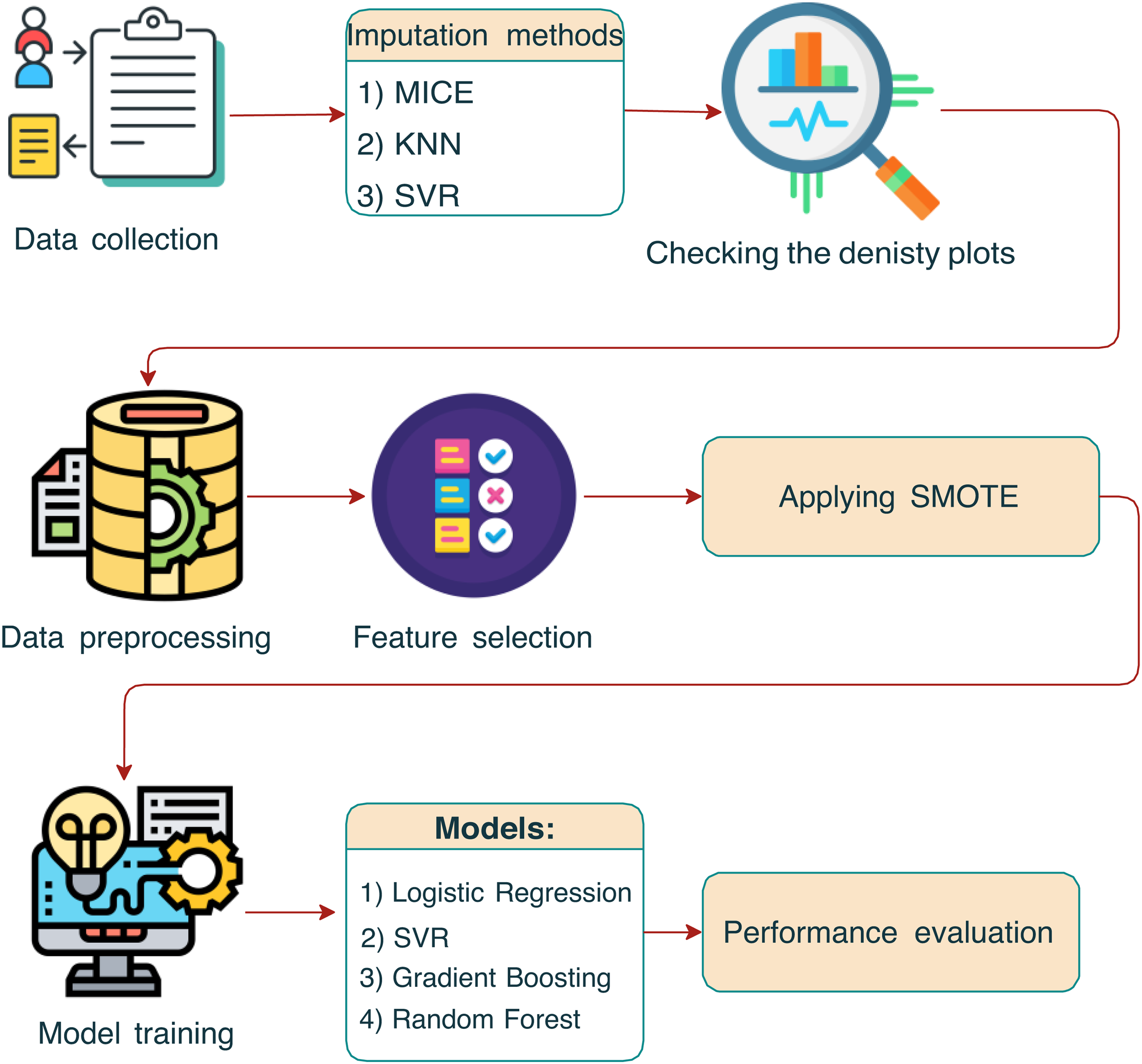
The schematic outlines the sequential steps from data collection through imputation, preprocessing, synthetic minority oversampling technique (SMOTE) application, and model training, to the final performance evaluation.

Dataset description

Data collection

The dataset was collected by researchers from the Institute of Human Convergence Health Science at Gachon University. The research was conducted in community settings in the city of Incheon, including social welfare centers, daycare centers, and senior welfare centers. The data were collected and analyzed over a nine-month period from 1 September 2022 to 31 May 2023. This period allowed wide sampling across many sites, thereby ensuring that the collected data covered all aspects of the study population. The study was conducted according to the guidelines of the Declaration of Helsinki and approved by the Gachon University Institutional Bioethics Committee (approval no. 1044396-202301-HR-020-01). All participants provided informed consent.

The dataset comprises health, physical, and lifestyle data from 664 participants, spanning a wide array of variables. The data collection process was performed following standardized protocols to ensure the accuracy and reliability of the measurements.

The dataset includes 97 variables categorized into demographic information, physical measurements, functional tests, medical assessments, and health conditions. The key variables include (refer to Table 1).

Table 1.

Overview of dataset variables.

Category	Variables
Demographics	Age, sex, place of data collection
Physical measurements	Height, weight, SMM,
	BFM, BMI,
	Percent body fat
Functional tests	Handgrip strength, plantar and dorsal flexion strength,
	Single-leg stance ability
Medical assessments	FVC, PreFVC,
	FEV1, PEF,
	MIP
Health conditions	Sleep disorder, DM,
	Hypertension, hyperlipidemia, hemoglobin A1c levels

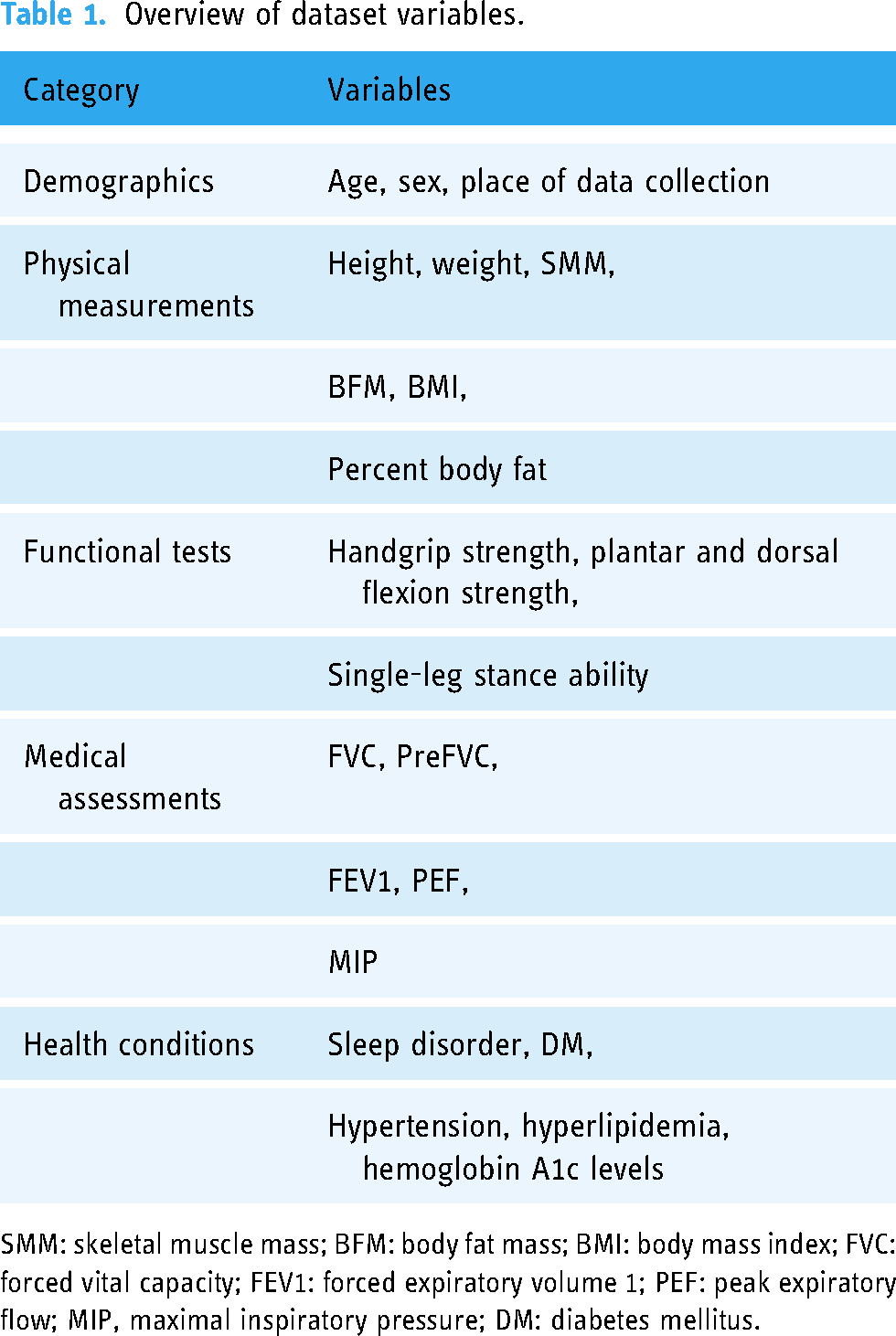
SMM: skeletal muscle mass; BFM: body fat mass; BMI: body mass index; FVC: forced vital capacity; FEV1: forced expiratory volume 1; PEF: peak expiratory flow; MIP, maximal inspiratory pressure; DM: diabetes mellitus.

Measurement criteria

Based on a systematic review of the existing literature on sarcopenia and following the AWGS guidelines, a comprehensive set of measurement items was selected to assess sarcopenia risk. The measurement criteria encompassed the following categories.

Physical fitness and muscle function tests:

Balance tests: Single-leg stance test to evaluate static balance.

Coordination tests: Timed up-and-go test to assess mobility and fall risk.

General physical function tests: These tests included balance tests, walking tests, and the sit-to-stand test to assess lower body strength and endurance.

Health fitness measurements:

Muscle strength: Handgrip strength was measured using a dynamometer and lower limb strength was assessed through the FET2 test.

Endurance: Endurance was evaluated through the sit-to-stand test.

Flexibility: Flexibility was assessed using the sit-and-reach test.

Cardiorespiratory endurance: This was measured by the two-minute step-in-place test.

Respiratory muscle measurements:

Maximal inspiratory pressure (MIP): To assess the strength of respiratory muscles.

Predicted forced vital capacity (FVC) and peak expiratory flow rate (PEF): To evaluate lung function and respiratory health.

Additional measurements:

Health and exercise capacity: These assessments included skin advanced glycation end-products, HbA1C levels to monitor blood sugar control, and overall exercise capacity.

Respiratory muscle strength: Assessed using devices such as spirometers to measure maximal inspiratory and expiratory pressures.

Each participant underwent a comprehensive evaluation, adhering to standardized protocols for each measurement item to ensure consistency and accuracy. In addition, the data collection process was performed by trained personnel to minimize errors and ensure participant safety.

Imputation methods

Multiple imputation by chained equations (MICE)

The MICE algorithm is an iterative method to impute missing data in a dataset with multiple variables. The process is described as follows:

Initialization: The algorithm begins by initializing the missing values, frequently using mean/mode imputation or random sampling from observed values.

Imputation step: For each variable $X_{i}$ with missing values, a regression model is fitted to the dataset, where $X_{i}$ is the dependent variable, and all other variables are treated as independent variables. The missing values of $X_{i}$ are then imputed using the fitted model. This step is repeated for each variable with missing data.

Iteration: The imputation and model-fitting steps are iterated multiple times. In each iteration, the models for each variable are updated using the latest imputed values from the previous iteration.

Mathematically, for a variable

X_{i}

, the imputation model at iteration

t

can be represented as follows:

X_{i}^{(t)} = β_{0} + \sum β_{j} X_{j}^{(t - 1)} + ϵ

(1)

where

X_{j}^{(t - 1)}

represents the imputed or observed values of other variables used as predictors in the model for

X_{i}

β_{j}

are the coefficients estimated from the regression, and

ϵ

is the error term.

SVR imputation

The SVR imputation method is a proficient technique to address the challenge of missing data within the sarcopenia dataset. By harnessing the capabilities of SVMs tailored to regression tasks, SVR imputation is adept at managing datasets characterized by nonlinear relationships and considerable dimensionality (these traits are frequently observed in healthcare datasets). The intrinsic strength of SVR imputation lies in its sophisticated modeling of intricate variable interactions, thereby enabling refined and precise replacement of missing values. Such precision maintains the integrity of the original data architecture and ensures the viability of subsequent statistical evaluations and the development of effective ML models. Thus, this methodological choice is instrumental in overcoming the obstacles posed by missing data, particularly in the complex and nuanced context of sarcopenia research.

SVR imputation is based on the principle of fitting a regression model that minimizes the error within a predefined epsilon margin. Formally, given a dataset with features $X$ and a target variable $y$ exhibiting missing values, SVR seeks to solve the following optimization problem:

min_{ω, b, ξ, ξ *} \frac{1}{2} ω^{T} ω + C \sum_{i = 1}^{n} (ξ_{i} + ξ_{i} *)

(2)

Subject to:

y_{i} - ω^{T} ϕ (X_{i}) - b \leq ϵ + ξ_{i},

(3)

ω^{T} ϕ (X_{i}) + b - y_{i} \leq ϵ + ξ_{i} *,

(4)

ξ_{i}, ξ_{i} * \geq 0, \forall i,

(5)

where

ϕ (X_{i})

represents the high-dimensional feature space mapped from the original inputs,

C

is the penalty parameter on the error term, and

ξ_{i}

ξ_{i} *

are slack variables that cater for data points outside the epsilon margin.

Implementing the SVR imputation method in healthcare datasets involves several key steps. First, the selection of an appropriate kernel function (e.g. linear, polynomial, and radial basis functions) and parameter tuning are crucial to capture the intricacies of the data. Then, the SVR model is trained on the available (non-missing) data using cross-validation to mitigate overfitting and ensure sufficient generalizability. Subsequently, the trained SVR model is applied to predict missing values, thereby generating a complete dataset for subsequent analysis. Finally, the impact of the imputation on downstream analysis is evaluated, and the model is refined iteratively as required to enhance accuracy.

Compared with traditional imputation methods, for example, mean/mode imputation, or regression-based techniques, SVR imputation offers several advantages. For example, it can effectively handle nonlinear relationships and high-dimensional data, both of which are prevalent in healthcare settings. In addition, by capturing the complex interactions between variables, SVR imputation ensures a more nuanced and accurate imputation of missing values, thereby preserving the underlying data structure and facilitating robust statistical analysis and ML model development.

KNN imputation

In the context of missing data in sarcopenia datasets, the KNN imputation method is an adept solution, especially when adhering to the MAR assumption. This premise suggests that the likelihood of data being missing in a variable is conditional on the observed data. A significant merit of KNN imputation for sarcopenia datasets is its straightforward approach and the minimal assumptions required concerning the distribution of the data. Thus, KNN imputation is a versatile and reliable method for the complex data structures typically encountered in healthcare research.

KNN imputation involves pinpointing the KNN to an observation of missing data and then using the values of these neighbors to impute the missing information. The determination of closeness between observations frequently employs different metrics, for example, the Euclidean or Manhattan distance. Specifically, the Euclidean distance between two points, $x$ and $y$ in an $n$ -dimensional space is computed as follows:

d (x, y) = \sqrt{\sum_{i = 1}^{n} (x_{i} - y_{i})^{2}}

(6)

With KNN imputation, the Euclidean distance helps identify the most analogous complete cases to the instance with missing data.

Implementing KNN imputation involves several pivotal steps. Initially, selecting the appropriate number of k neighbors is essential, which is frequently determined using cross-validation to optimize the bias-variance trade-off. Then, the distance between each pair of complete and incomplete cases is calculated using the chosen metric. For each instance of missing data, either the average (for continuous variables) or the mode (for categorical variables) of the values of the KNN is computed and used for imputation.

Despite potential limitations, KNN imputation is a viable strategy to manage missing data in sarcopenia datasets under MAR conditions. Ismail et al.²³ highlighted the method’s robustness and simplicity, noting its superior performance over various ML imputation techniques. In addition, its ease of implementation contributes to its accessibility for both researchers and practitioners. The apparent simplicity of KNN imputation masks its efficacy in addressing the intricacies of medical data, thereby making it an effective option for diverse healthcare data challenges.

KNN imputation is a valuable method within the spectrum of techniques utilized to address missing data in healthcare datasets. Its straightforward nature and effectiveness position it competitively among more intricate algorithms, particularly in scenarios characterized by the MAR mechanism. Nonetheless, it is imperative to perform a thorough assessment of the dataset’s specific attributes and the interrelations among variables to identify the most appropriate imputation strategy because certain contexts may require more sophisticated methods.

Comparison of density plots

In the absence of the original dataset, post-imputation density plot comparisons allow us to evaluate the implications of various imputation methodologies on the distribution of the data. Imputation demands rigorous assessment to ensure the preservation of data integrity. Density plots, representing the distribution of data, facilitate effective visual comparisons of the effects of different imputation techniques on the distributional characteristics of the data, including shape, spread, and central tendency. Notable deviations in these post-imputation density plots could signify the introduction of bias or alterations to the underlying data structure, whereas negligible variations may indicate the effective preservation of the original data characteristics. Thus, this comparative technique is a pivotal academic exercise that provides valuable insights into the efficacy of imputation methods and their impact on subsequent statistical analysis and model accuracy, thereby guiding researchers toward the most appropriate imputation strategies to uphold the analytical integrity of their studies.

The evaluation of imputation techniques using density plot comparisons provides a visual and statistical approach to assess the similarity between the distributions of observed and imputed data. This approach is crucial when handling missing data in datasets with MAR mechanisms. Adopting an imputation model that generates a density of imputed values most similar to the observed values.²⁴ Using stable balancing weights to compare the density of imputed and observed values, illustrating this approach using various imputation methods, including predictive mean matching and multivariate normal imputation.

In addition, density plot comparisons help evaluate imputation methods based on their ability to maintain the original data structure and yield lower imputation errors. A method that combines nearest neighbor estimation and density estimation with Gaussian kernels for imputation has demonstrated promising results in maintaining the complexity of the original data structure compared to current methods.²⁵

To implement density plot comparisons, one would typically follow the following steps.

Impute missing data by applying various imputation techniques to the dataset with missing values.

Generate density plots for both the original dataset (without missing values) and the imputed datasets.

Perform a visual comparison of the plots to assess how well the imputed data distribution aligns with the distribution of the original data.

Visual comparison:

Overlay the density plots of the original (observed) data and the imputed data.

Evaluate the similarity in the shape, central tendency, and spread of the distributions.

Identify significant deviations or discrepancies between the compared distributions.

This approach ensures that the selected imputation method provides the most accurate reflection of the original data distribution, thereby preserving the integrity of the data for further analysis. In addition, a significant advantage of using density plots lies in their ability to represent the data distribution graphically, which facilitates an intuitive comparison of the effectiveness of different imputation methods. Thus, density plot comparisons serve as a practical and informative tool to evaluate imputation techniques, particularly when handling datasets that contain missing data under the MAR assumption.

Data preprocessing

Normalization, particularly min–max normalization, is crucial for processing a sarcopenia dataset to ensure uniformity in scale across various measurements, thereby enhancing the comparability and performance of analytical models. This method transforms features to a common scale between 0 and 1 as follows:

x_{norm} = \frac{x - x_{min}}{x_{max} - x_{min}}

(7)

Here,

x

is the original value, and

x_{min}

and

x_{max}

are the minimum and maximum values of the feature, respectively. Such normalization is essential for sarcopenia research because it mitigates the effects of varying measurement units and magnitudes, thereby facilitating accurate comparisons and integrations of data points from diverse sources. This process streamlines data analysis and improves the efficiency and accuracy of predictive modeling efforts.

Feature selection

To identify the key factors contributing to sarcopenia, this study employed correlation analysis and visual examinations to select relevant features from the dataset. Initially, a correlation matrix was calculated to discern the linear relationship of all available features with the target variable “sarcopenia_2,” where a value of zero indicates the absence of sarcopenia, and a value of one indicates the presence of the disease. This analytical step is critically important because it enables the identification of variables that exhibit significant linear associations with the target condition of interest, thereby shedding light on potential predictors or risk factors of sarcopenia.

Following the computation of the correlation matrix, we focused on sorting the correlation coefficients associated with the “sarcopenia_2” variable by arranging them in descending order. This process highlighted the features with the strongest positive linear relationships and those with notable negative correlations, which provided a comprehensive overview of how each feature may influence the likelihood or severity of sarcopenia.

Further refining the feature selection process, we established a correlation threshold of 0.3 to filter out features with weaker linear relationships with the “sarcopenia_2” variable (Table 2). This threshold was selected to ensure that only features with at least a moderate (positive or negative) correlation were considered in the subsequent analyses. By applying this criterion, we excluded the target feature itself and compiled a list of features that met or exceeded the threshold. The final selection encompassed a precise number of features that surpassed the correlation threshold and excluded redundant or irrelevant variables, thereby optimizing the dataset for more focused and efficient analysis (Figure 2).

Figure 2.

Highly correlated features with “Sarcopenia_2.”

Table 2.

The selected features.

ID	Features	Meaning
1	SARC_CalF	Sarcopenia self-diagnosis questionnaire + calf circumference
2	G_HG_R	Grade of right hand grip
3	G_HG_L	Grade of left hand grip
4	Age	Age of the participant
5	SS_SPPB	Stand and sit (SPPB)
6	G_TUG	Grade of timed up and go
7	Plantar_R_1	Plantar flexion, calf muscle strength right, one time
8	D_Plantar	Dominant plantar flexion
9	PEF	Peak expiratory flow
10	ND_Plantar	Nondominant plantar flexion
11	Plantar_L_1	Plantar flexion, calf muscle strength left, one time
12	ND_Dorsal	Nondominant dorsal flexion
13	Dorsal_L_1	Calf muscle strength left, one time for dorsal flexion
14	height_cm	Measurement of a person’s height in centimeters
15	Dorsal_R_1	Calf muscle strength right, one time for dorsal flexion
16	FEV1	Forced expiratory volume in one second
17	D_Dorsal	Dominant dorsal flexion
18	SPPB	Short physical performance battery test
19	BFM_kg	Body fat mass in kilograms
20	G_BMI	Grade of body mass index
21	BMI_kgm2	Body mass index in kg/m $^{2}$
22	HG_L_1	Hand grip left 1 time
23	ND_HG	Nondominant hand grip
24	HG_R_1	Hand grip right 1 time
25	HG_L_M	Hand grip left maximum
26	HG_L_2	Hand grip left 2 times
27	HG_R_M	Hand grip right maximum
28	HG_R_2	Hand grip right 2 times
29	SMM_kg	Skeletal muscle mass in kilograms
30	D_HG	Dominant hand grip
31	BMR_kcal	Basal metabolic rate in kcal
32	CC_cm	Calf circumference
33	weight_kg	Person’s body weight measured in kilograms
34	ASM	Appendicular skeletal muscle

Synthetic minority oversampling technique (SMOTE)

The SMOTE technique is frequently used to address class imbalance in datasets, particularly in supervised learning tasks. The objective of SMOTE is to generate synthetic instances of the minority class by interpolating between existing minority instances and their nearest neighbors. This oversampling approach attempts to balance the class distribution, thereby improving the performance of classification algorithms on imbalanced datasets.

Mathematically, for each minority instance $x$ , SMOTE selects its KNN from the minority class. Then, synthetic instances are generated along the line segments joining $x$ and its KNN as follows:

x_{new} = x + λ * (x_{nn} - x)

(8)

where

x_{nn}

is a randomly selected nearest neighbor, and

λ

is a random number between 0 and 1.

The SMOTE method effectively increases the decision region for the minority class, which enables the classifier to better capture the underlying distribution and decision boundaries. However, SMOTE should be employed judiciously because excessive oversampling may lead to overfitting and potential degradation of generalizability.

When employing SMOTE in ML, especially for imbalanced datasets, it is essential to recognize its potential limitations and biases introduced by the synthetic data generation process. These issues can impact model performance and generalizability.

Over-generalization: SMOTE creates synthetic samples by interpolating between minority class points and their nearest neighbors. This can lead to over-generalization, where synthetic samples are generated near the boundaries of the majority class. This blending of classes can introduce noise, reducing classification performance on test data.²⁶

Noisy data amplification: SMOTE can inadvertently amplify noisy or outlier data by synthesizing new instances around these points. This increases the risk of misclassification, as the model may learn spurious patterns rather than real trends.²⁷

Dimensionality challenges: In high-dimensional datasets, the synthetic data generated by SMOTE may not be effective in reducing the bias toward the majority class. SMOTE struggles to preserve the complex relationships in high-dimensional feature spaces, leading to lower predictive accuracy without feature selection.²⁸

Synthetic data instability: SMOTE’s random interpolation mechanism can lead to inconsistent outcomes depending on the choice of neighbors. Different runs of SMOTE can yield varying synthetic data and thus fluctuating model performance, which poses challenges in reproducibility and model validation.²⁹

Model training

The selection of the LR, GB, SVM, and RF models for training in the sarcopenia prediction context, which requires a binary outcome, is grounded in a blend of theoretical robustness, empirical performance, and model interpretability, all of which are vital to address complex datasets, for example, the experimental dataset utilized in this study.

Logistic regression provides a probabilistic framework that is suitable for binary classification tasks, for example, predicting sarcopenia, thereby offering interpretability and serving as a baseline model. GB models complex nonlinear relationships, which provides insights into feature importance, and is robust against overfitting. SVM methods model nonlinear boundaries using kernel functions, maximize margins for generalization and are effective in high-dimensional spaces. The RF method leverages an ensemble of decision trees, handles imbalanced data, and offers feature selection and importance evaluation, which are crucial for understanding the factors that contribute to sarcopenia.

Logistic regression

Logistic regression is a statistical model used for binary classification tasks, where the outcome variable is categorical and represents the probability of the occurrence of a specific event. Logistic regression methods model the log-odds of the dependent variable as a linear combination of the independent variables, where the logistic function is employed to ensure the output lies between 0 and 1. Mathematically, the probability of the event occurring is calculated as follows:

P (Y = 1) = \frac{1}{1 + e^{- (β_{0} + β_{1} X_{1} + . . . + β_{k} X_{k})}}

(9)

where

P (Y = 1)

is the probability of the event occurring,

e

is the base of the natural logarithm,

X_{1}, \dots, X_{k}

are the independent variables, and

β_{0}, β_{1}, \dots, β_{k}

are the coefficients representing the relationship between each independent variable and the log-odds of the dependent variable. Logistic regression is favored for its simplicity, interpretability, and direct estimation of the odds ratios, which makes it an effective choice for binary classification problems in various fields.

3.7.2. Gradient boosting

GB is a powerful ensemble ML technique that builds predictive models in a stage-wise fashion by focusing on correcting the errors of previous models by adding new models that address these errors directly. In the healthcare context, particularly for predicting sarcopenia, GB leverages a series of decision trees to improve predictions iteratively. The core concept is encapsulated in the following expression:

F_{m} (x) = F_{m - 1} (x) + ρ_{m} h_{m} (x)

(10)

where

F_{m} (x)

is the model at iteration

m

h_{m} (x)

is the decision tree added at the

m

th step, and

ρ_{m}

is the learning rate. For a sarcopenia dataset, GB begins with a base model (frequently a simple decision tree) and iteratively adds trees that predict the residuals of the previous model, thereby improving the accuracy of the sarcopenia predictions. In addition, training involves selecting loss functions pertinent to classification or regression tasks, for example, logistic loss for the binary classification of sarcopenia presence. By tuning the relevant parameters, for example, the number of trees, tree depth, and learning rate, the GB method adaptively learns complex patterns that are indicative of sarcopenia from clinical and physiological data, thereby making it a robust tool for healthcare analytics.

Support vector machine (SVM)

The SVM is a supervised learning model known for its effectiveness in classification tasks, including sarcopenia detection. An SVM operates on the principle of finding the optimal hyperplane that maximizes the margin between two classes, encapsulated by:

y_{i} (w \cdot x_{i} + b) \geq 1 - ξ_{i}

(11)

where

w

is the weight vector,

x_{i}

are the feature vectors,

b

is the bias,

y_{i}

are the class labels, and

ξ_{i}

are the slack variables allowing for margin violations. The SVM utilizes kernel functions to enable nonlinear classification, which is crucial for complex health datasets (such as those involving sarcopenia), where linear separation in the original feature space may be infeasible. Training an SVM model on a sarcopenia dataset involves selecting a kernel (e.g. a linear, polynomial, or radial basis function kernel) and parameter tuning (e.g.

C

and other kernel-specific parameters) through cross-validation to optimize the model’s ability to distinguish between sarcopenia-affected and healthy subjects, based on clinical indicators and patient characteristics. Their robustness, ability to handle high-dimensional data, and effectiveness in binary classification tasks make SVM models suitable for advancing sarcopenia research and diagnostics in healthcare.

3.7.4. Random forest (RF)

The RF technique is an ensemble learning method that excels in classification tasks. This method constructs multiple decision trees during the training phase and outputs the mode of the classes (classification) of the individual trees. The fundamental principle of the RF method is the improvement of prediction accuracy by reducing overfitting, which is achieved through bagging (bootstrap aggregating) and feature randomness when splitting nodes, which is expressed as follows:

f (x) = \frac{1}{N} \sum_{i = 1}^{N} T_{i} (x; Θ_{i})

(12)

where

T_{i} (x; Θ_{i})

denotes the

i

th tree’s prediction for input

x

with randomness

Θ_{i}

, and

N

is the number of trees. For sarcopenia datasets, training involves generating a diverse set of trees on bootstrapped samples of the data and employing measures, for example, Gini impurity or entropy, to select the split points. This allows the RF method to handle complex, multidimensional data effectively, thereby making it highly suitable for identifying patterns indicative of sarcopenias, for example, muscle mass decline and strength reduction, from a broad set of predictors, including patient demographics, physical activity levels, and medical history. Its robust performance, ease of use, and interpretability make the RF method a potent tool for sarcopenia research and other healthcare-related classification tasks.

K-fold cross-validation

K-fold cross-validation is a robust technique to evaluate the generalizability of a model and present overfitting. During model training, 10-fold cross-validation is performed using the K-fold class from sklearn.model_selection. Here, the dataset is partitioned into 10 equal folds, and the model is trained and evaluated 10 times, with each fold serving as the validation set once. The cross_val_score function computes the accuracy score for each fold, and the mean accuracy across all folds is reported to provide an estimate of the model’s performance on unseen data. The K-fold cross-validation estimate of a metric $M$ is calculated as follows:

M = \frac{1}{k} \sum_{i = 1}^{k} M_{i},

(13)

where

M_{i}

is the metric computed on the

i

th validation fold. Note that cross-validation is crucial for reliable model evaluations, particularly with limited data, because it maximizes data utilization for training and validation, thereby mitigating overfitting and providing a more robust performance estimate.

Model performance measurement

A combination of evaluation metrics that provide insights into a model’s effectiveness, for example, precision, recall, F1-score, and accuracy, is frequently used to evaluate the performance of a classification model. Each of these metrics serves a specific purpose and offers valuable information about the model’s predictive capabilities.

Precision is the ratio of correctly predicted positive observations to the total number of predicted positive observations. Precision is expressed as follows:

Precision = \frac{TP}{TP + FP}

(14)

Note that a high precision value indicates a low false-positive rate, which is desirable in many applications.

Recall (also referred to as sensitivity) measures the ratio of correctly predicted positive observations to all observations in an actual positive class. Recall is calculated as follows:

Recall = \frac{TP}{TP + FN}

(15)

A high recall value implies a low false-negative rate, which ensures that the model captures the most positive instances.

The F1-score is the harmonic mean of precision and recall. It attempts to achieve a balance between precision and recall by considering both metrics. The F1-score is calculated as follows:

F1-score = 2 \cdot \frac{Precision \cdot Recall}{Precision + Recall}

(16)

Note that an F1-score of one indicates a perfect balance between precision and recall, and a score of zero represents a complete failure to achieve an effective balance.

Accuracy, which represents the ratio of correctly predicted observations to the total number of observations, is the most intuitive performance measure. Accuracy is calculated as follows:

Accuracy = \frac{TP + TN}{TP + TN + FP + FN}

(17)

Note that accuracy provides an overall measure of correctness; however, it may not be sufficient for imbalanced datasets or when the costs of false positives and false negatives differ.

Collectively, these metrics provide a comprehensive evaluation of the model’s performance. Precision and recall highlight the model’s ability to minimize false positives and false negatives, respectively, and the F1-score balances these two metrics. Accuracy provides an effective overall measure of correctness. The choice of metrics to prioritize depends on the specific application and the relative importance of different types of errors.

Computational environment

To ensure experimental reproducibility, all experiments were conducted using Kaggle notebooks. This cloud-based platform provides a standardized computational environment with pre-installed libraries commonly used in data science and ML tasks. For transparency and to facilitate replication, the source code for our implementation is available on GitHub (https://github.com/dilmurod86/Sarcopenia_Imputation.git).

Results

Dataset missingness

When we analyzed the degree of missingness in the sarcopenia dataset, we obtained the following results (Table 3).

Table 3.

Categorization of dataset features by level of missingness.

Missingness category	Number of features
0%	18
>0% to 5%	11
>5% to 10%	1
>10% to 20%	0
>20% to 30%	60
>30% to 40%	7

Complete observations (0% missingness): Eighteen features exhibited no missing data, which indicate a robust set of variables with complete observations. This category represents the most reliable subset of the dataset, unaffected by the challenges of missing data imputation.

Minimal missingness (0% to 5%): Here, 11 features fell within this minimal range of missingness, displaying a negligible level of incomplete data. Note that the slight missingness in these features is unlikely to significantly impact analytical outcomes, thereby allowing for straightforward handling using common imputation techniques or complete case analysis.

Low missingness (5% to 10%): A singular feature was identified with missingness slightly above 5% but not exceeding 10%, marking a high level of data completeness. This feature, requiring minimal imputation, can be integrated effectively into analytical models with little concern for bias introduced by the missing data.

Moderate missingness (20% to 30%): Here, 60 features were characterized by missingness levels between 20% and 30%. This considerable segment of the dataset presents a moderate challenge for data analysis, requiring thoughtful application of imputation methods or utilization of analytical techniques that are robust against missing data.

Severe missingness (30% to 40%): Seven features were identified with >30% of their data missing, which represents severe missingness. These features require special attention because standard imputation methods may be insufficient to address the extensive gaps in the data. Advanced statistical techniques, including model-based imputation or the use of algorithms designed to handle large proportions of missing data, may be required to utilize these variables effectively in analysis.

Comparison of density plots

Figure 3 compares the performance of three different imputation techniques on two variables, that is, “CC_cm”(20% missingness) and “HG_R_2”(30% missingness) under varying missingness conditions. Here, each plot pairs the original data distribution (before imputation) with the imputed data distribution, which allows us to perform a post-imputation evaluation of the preservation of statistical properties.

Figure 3.

Comparative density plots of CC_cm and HG_R_2 variables before and after imputation using MICE, SVR, and KNN techniques, with missingness levels of 20% and 30%, respectively. MICE: multiple imputation by chained equations; SVR: support vector regression; KNN: k-nearest neighbors.

The MICE algorithm, which is a multivariate technique, is frequently preferred when handling complex datasets with patterns that simpler models may not capture. For the “CC_cm” feature, MICE imputation closely mirrors the original distribution, maintaining both the central tendency and variability. In addition, the “HG_R_2” feature also exhibits a high degree of overlap between the original and imputed distributions, which suggests that the MICE algorithm handles higher levels of missingness effectively without significant distortion.

The SVR method is particularly adept at capturing nonlinear relationships in data, which is crucial for features with underlying patterns that are not well represented by linear models. The SVR imputation for the “CC_cm” feature shows a minor deviation in peak density, which indicates a slight alteration in the central tendency or variance after imputation. However, the “HG_R_2” feature maintains high fidelity to the original distribution, thereby indicating SVR’s robust performance even with 30% missing data.

The KNN method relies on feature similarity, and it assigns missing values based on the resemblance to their nearest neighbors. For the “CC_cm” feature, the KNN method exhibits a close approximation to the original dataset, which suggests effective imputation was realized within a local structure of the data. Conversely, the plots for the “HG_R_2” feature reveal a marginal difference, particularly in the tails, potentially reflecting the influence of the chosen “k” or distance metric on the imputation quality.

Across all compared methods, the plots indicate satisfactory retention of the key characteristics of the original distributions. The MICE algorithm stands out for its robustness, especially for the “HG_R_2” feature, which had a higher degree of missingness. The SVR method exhibits strong performance, with slight variations possibly reflecting its sensitivity to parameter tuning. The KNN method, while generally consistent, highlights the need for careful neighbor selection to avoid deviations in tail areas, particularly in datasets with a significant proportion of missing data.

SMOTE technique

In the context of classifying sarcopenia presence within a dataset, the SMOTE was utilized to address class imbalance. Prior to applying SMOTE, the dataset exhibited a significant disparity between the majority class “0,” indicating the absence of sarcopenia ( $n = 419$ ), and the minority class “1,” representing the presence of sarcopenia ( $n = 112$ ). This imbalance can lead to a bias toward the majority class in predictive modeling.

After applying the SMOTE method, the minority class was augmented to match the majority class, with both classes reflecting an equal count of 419 instances. This oversampling of the minority class was performed by generating synthetic samples rather than a simple duplication of existing samples. By promoting balance in the class distribution, SMOTE enhances the generalizability and performance of classifiers in predicting the less represented class, which, in this case, is the presence of sarcopenia.

Here, the use of SMOTE is crucial in terms of developing a more robust and accurate classification model, thereby improving the identification and subsequent intervention strategies for sarcopenia within the target population (Figure 4).

Figure 4.

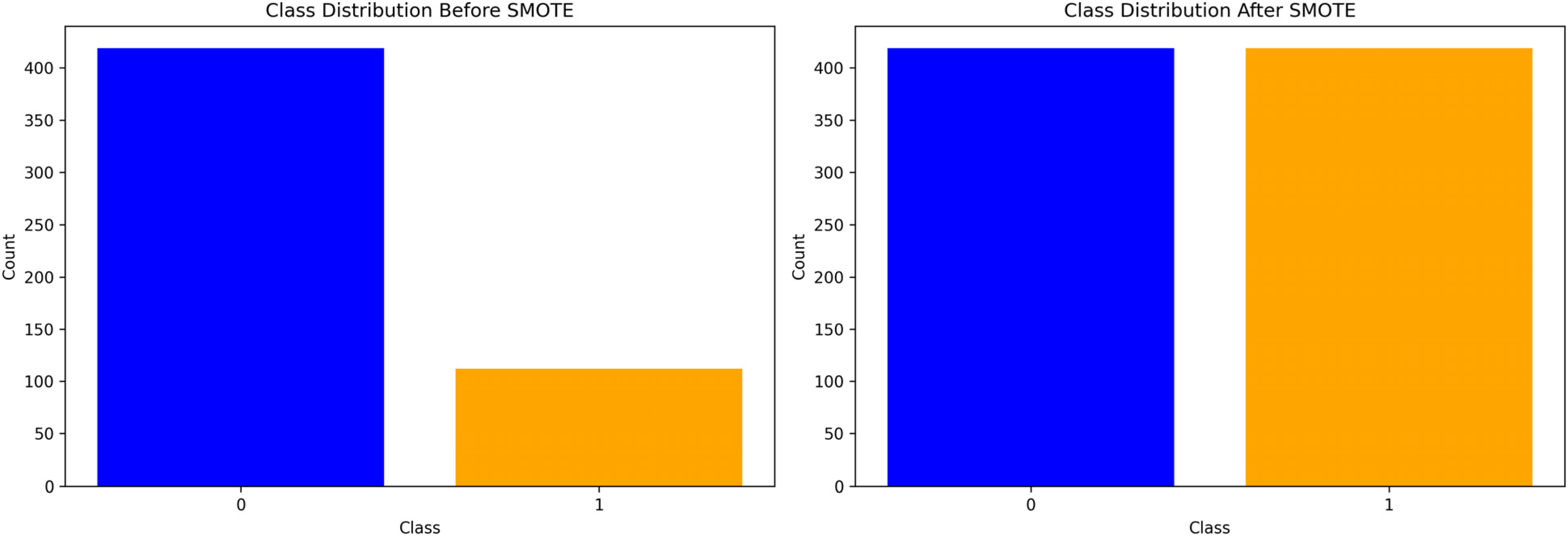
Bar graphs depicting the class distribution for sarcopenia detection before and after applying synthetic minority oversampling technique (SMOTE).

Comparison of model performance

The comparative analysis of model performance involved the application of three distinct imputation techniques, that is, the MICE, SVR, and KNN methods, to rectify missing data in the datasets. Then, several predictive models, including LR, GB, SVM, and RF models were trained. Here, two sets of results were generated, where one set was based on the initial test dataset, and the other set was obtained following a rigorous 10-fold cross-validation process.

The accuracy results (Table 4) obtained on the test dataset provided initial insights into the post-imputation performance of the models. For the KNN-imputed dataset, both the LR and SVM models achieved an accuracy of 0.934, which indicates strong predictive capabilities. In addition, the GB and RF models performed equally with an accuracy of 0.970. On the MICE-imputed dataset, the LR and RF models exhibited identical accuracy of 0.970, surpassing that of the SVM model (0.922). The GB model also obtained a high accuracy of 0.970. In contrast, on the SVR-imputed dataset, the GB model demonstrated the highest accuracy of 0.982, and the RF, SVM, and LR models obtained accuracy values of 0.964, 0.910, and 0.898, respectively.

Table 4.

Results for the test dataset.

	KNN	MICE	SVR
LR	0.934	0.922	0.898
SVM	0.934	0.922	0.910
GB	0.970	0.970	0.982
RF	0.970	0.970	0.964

KNN: k-nearest neighbors; MICE: multiple imputation by chained equations; SVR: support vector regression; LR: logistic regression; SVM: support vector machine; GB: gradient boosting; RF: random forest.

Note that a nuanced shift in model performance was observed after applying 10-fold cross-validation to mitigate overfitting and assess model stability. The results are shown in Table 5. Here, the KNN-imputed dataset yielded slightly reduced accuracy with the LR model (0.926) and a modest increase with the RF model (0.974), while the SVM and GB models remained consistent at 0.932 and 0.982, respectively. The MICE imputation technique’s cross-validated results indicated superior consistency across the compared models, with the LR, SVM, GB, and RF models achieving accuracy values of 0.928, 0.937, 0.979, and 0.974, respectively. Here, after cross-validation, the SVR imputation technique sustained high performance for all models, particularly the GB model, which obtained an accuracy value of 0.979, and the RF model (0.968). In addition, the LR and SVM models obtained an equal accuracy of 0.928.

Table 5.

Results after 10-fold cross-validation.

	KNN	MICE	SVR
LR	0.926	0.928	0.928
SVM	0.932	0.937	0.938
GB	0.982	0.979	0.979
RF	0.974	0.974	0.968

Discussion

Based on the statistical analysis of the imputation methods (Table 6), we found that the KNN method realized better reliability and consistency in terms of model performance, obtaining a high mean accuracy of 0.952 and a low standard deviation of 0.0208, with a 95% confidence interval ranging from 0.934 to 0.970; thus, the KNN imputation method is both stable and dependable. In contrast, the MICE method obtained a mean accuracy of 0.946 and slightly greater variability, as indicated by the somewhat larger standard deviation than the KNN method. Performance estimates for the MICE method demonstrate moderate precision compared with the KNN method. The SVR method obtained a mean value for the lowest accuracy: of 0.9385, a standard deviation of 0.0408, and a wide confidence interval of 0.904, 0.9775, indicating considerable variability and uncertainty in its performance. The results also show that the KNN method was the most reliable imputation technique for the target sarcopenia data, followed by the MICE algorithm as a reasonable alternative. The SVR was found to be the least stable method, which is not favorable for the target task.

Table 6.

Performance of models with different imputation methods.

Imputation	Mean accuracy (SD)	95% CI
KNN	0.952 (0.021)	(0.934, 0.970)
MICE	0.946 (0.028)	(0.922, 0.970)
SVR	0.939 (0.041)	(0.904, 0.978)

SD: standard deviation; KNN: k-nearest neighbors; MICE: multiple imputation by chained equations; SVR: support vector regression.

Collectively, the results obtained on the test and cross-validated datasets underscore the impact of the imputation techniques on model performance. There is evidence of a discrepancy in accuracy between the models when subjected to different imputation strategies, which emphasizes the importance of selecting an appropriate imputation method to optimize predictive accuracy. The cross-validation results further solidify the robustness of the models, providing a comprehensive understanding of their performance when handling imputed datasets.

The evaluation of the models’ predictive performance, differentiated by the absence (class 0) and presence (class 1) of sarcopenia, was conducted utilizing the precision, recall, and F1-score metrics. These metrics were computed after applying the MICE, KNN, and SVR imputation methods to the datasets.

Here, the precision, recall, and F1-score metrics were calculated for the LR, SVM, GB, and RF classifiers. The results are shown in Tables 7 and 8. As can be seen, the LR and SVM models obtained high precision values for the negative class (0) at 0.95 and equally strong recall values for the positive class (1) at 0.96. However, the GB model exhibited perfect precision and recall for both classes, mirrored in an F1-score of 0.97, which indicates exceptional model performance. The RF model also obtained high precision and recall values, with an F1-score of 0.97 for both classes.

Table 7.

Model evaluation metrics by class based on the MICE imputation dataset.

Class	Precision	Recall	F1-score
LR
0	0.95	0.89	0.92
1	0.90	0.96	0.93
SVM
0	0.95	0.89	0.92
1	0.90	0.96	0.93
GB
0	1.00	0.94	0.97
1	0.95	1.00	0.97
RF
0	1.00	0.94	0.97
1	0.95	1.00	0.97

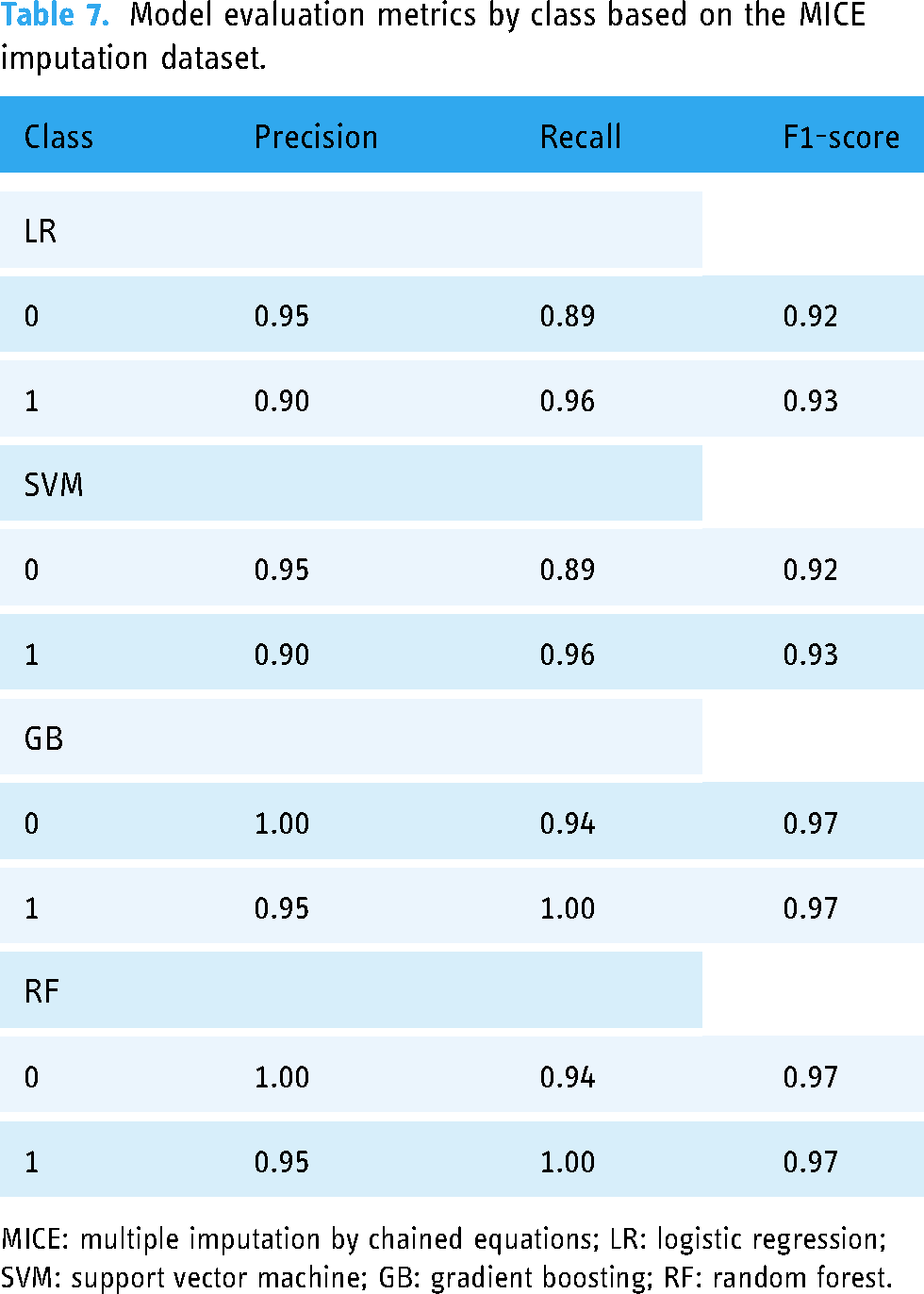
MICE: multiple imputation by chained equations; LR: logistic regression; SVM: support vector machine; GB: gradient boosting; RF: random forest.

Table 8.

Model evaluation metrics by class based on the KNN imputation dataset.

Class	Precision	Recall	F1-score
LR
0	0.97	0.89	0.93
1	0.91	0.98	0.94
SVM
0	0.97	0.89	0.93
1	0.91	0.98	0.94
GB
0	1.00	0.94	0.97
1	0.95	1.00	0.97
RF
0	0.99	0.95	0.97
1	0.96	0.99	0.97

KNN: k-nearest neighbors; LR: logistic regression; SVM: support vector machine; GB: gradient boosting; RF: random forest.

After applying the KNN imputation technique, the LR model exhibited a precision value of 0.97 for the negative class and 0.91 for the positive class, with recall scores closely matching at 0.89 and 0.98, respectively. The results of the SVM model were comparable to those of the LR model, showing balanced precision and recall values across the two classes. The GB model maintained high precision and recall, with an F1-score of 0.97 for both classes, and the RF model mirrored the GB model in terms of precision but exhibited slightly increased recall, maintaining an F1-score of 0.97 across both classes.

On the dataset imputed by the SVR method (Table 9), the LR model obtained precision scores of 0.93 for class 0 and 0.88 for class 1, with corresponding recall scores of 0.85 and 0.94. The SVM model obtained slightly reduced precision values for both classes compared to the LR model; however, the SVM model demonstrated improved recall, especially for the positive class at 0.97. The GB model obtained perfect precision for the negative class and high precision for the positive class, with recall being consistent at 0.96, with an F1-score of 0.98 for both classes. The RF model obtained high metrics across the board, with precision and recall values resulting in an F1-score of 0.97 for both classes.

Table 9.

Model evaluation metrics by class based on the SVR imputation dataset.

Class	Precision	Recall	F1-score
LR
0	0.93	0.85	0.89
1	0.88	0.94	0.91
SVM
0	0.93	0.87	0.90
1	0.89	0.94	0.92
GB
0	1.00	0.96	0.98
1	0.97	1.00	0.98
RF
0	0.97	0.95	0.96
1	0.96	0.98	0.97

SVR: support vector regression; LR: logistic regression; SVM: support vector machine; GB: gradient boosting; RF: random forest.

These metrics elucidate the impact of different imputation techniques on model performance. Notably, the GB model obtained consistently high precision and recall values with all imputation methods, which suggests its robustness when handling imputed datasets. In contrast, the LR and SVM models demonstrated variability in their performance, which may be influenced by the underlying imputation technique. The consistently high F1-score values across the compared models obtained on the dataset imputed by the SVR method underscore the significance of the imputation process in terms of model reliability and predictive accuracy.

Confusion matrices were generated for the LR, SVM, GB, and RF models with the SVR, MICE, and KNN imputation methods. These matrices are critical for evaluating the classifiers’ predictive accuracy by displaying the true positive, false positive, true negative, and false negative predictions.

With MICE imputation, the performance of the LR classifier was improved slightly with 70 true positives and 85 true negatives. The SVM classifier echoed this result with identical true positive and true negative counts. The GB model exhibited a slight reduction in performance with 74 true positives; however, it maintained a strong true negative prediction rate of 89. The RF classifier reflected a true positive count of 79 and a true negative count of 93, thereby demonstrating balanced accuracy across both the positive and negative predictions (Figure 5).

Figure 5.

Confusion matrices for logistic regression, support vector machine, gradient boosting, and random forest models after applying multiple imputation by chained equations (MICE) imputation technique.

The KNN imputation results were consistent with the MICE results for the LR and SVM classifiers, both reporting 70 true positives and 87 true negatives, thereby indicating a modest increase in the true negative predictions. The GB classifier exhibited a slight decline in true positive predictions to 74 but maintained a consistent count of 89 true negatives. In addition, the RF classifier maintained its performance with a true positive rate of 75 and increased its true negative predictions to 93 (Figure 6).

Figure 6.

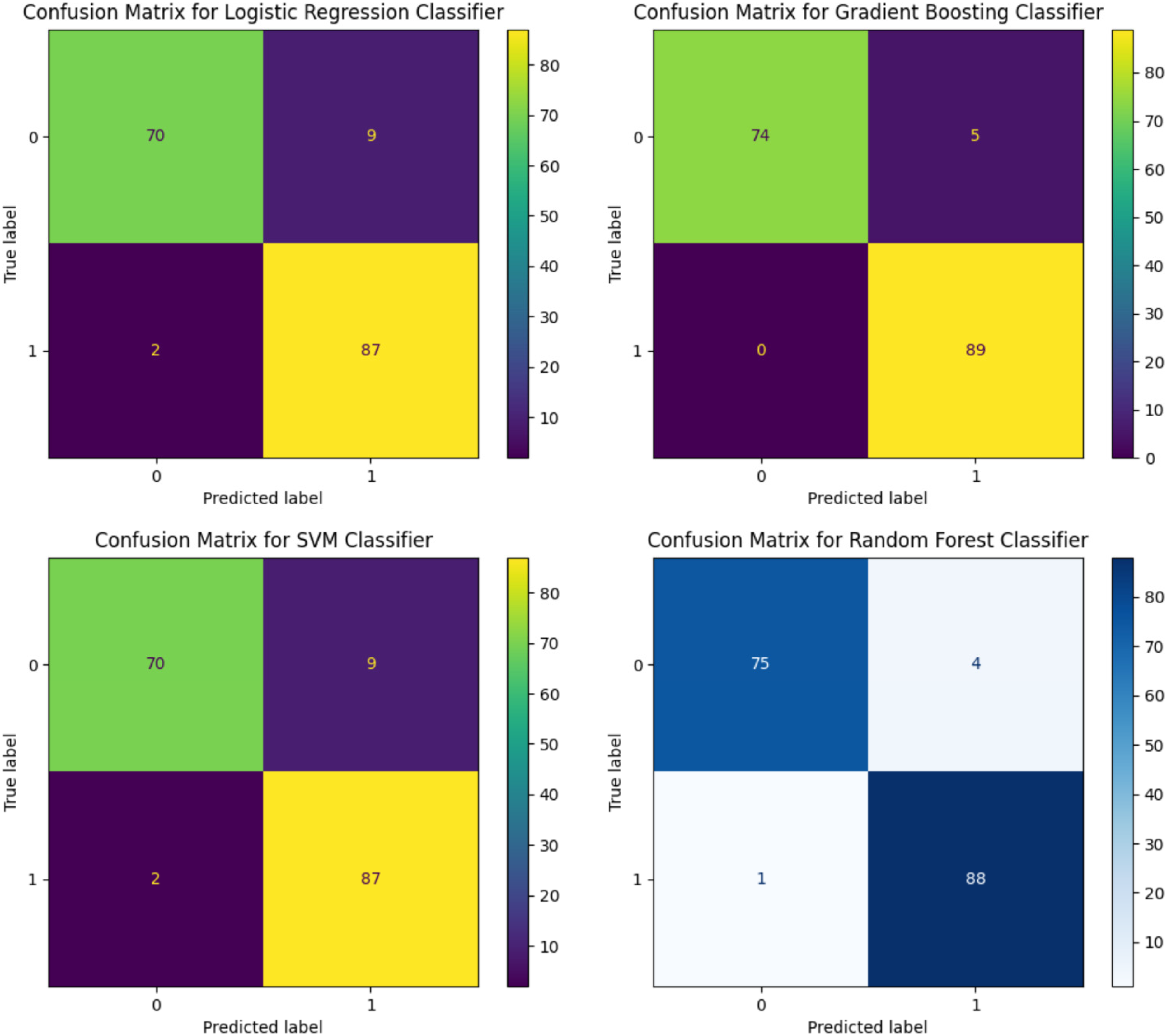
Confusion matrices for logistic regression, support vector machine, gradient boosting, and random forest models after applying k-nearest neighbors (KNN) imputation technique.

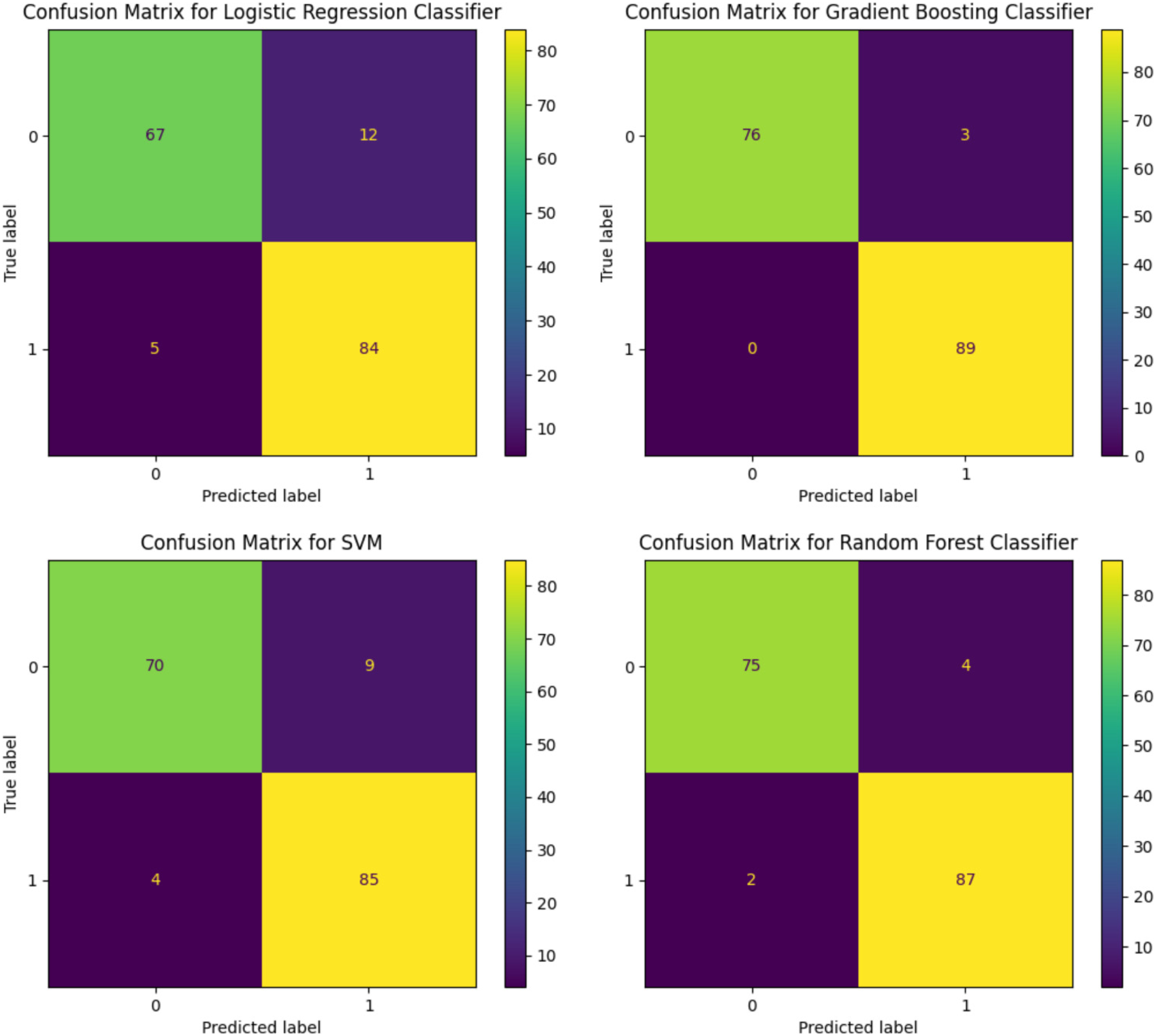
For the SVR imputation, the confusion matrix for the LR classifier exhibited 67 true positives and 94 true negatives, which indicates robust prediction for negatives. In contrast, the confusion matrix for the SVM classifier exhibited similar true positive predictions (69) but a marginally higher count of true negatives (94). The GB classifier demonstrated a higher propensity for correct positive predictions with 76 true positives and nearly flawless performance with 89 true negatives. The RF classifier, while achieving a lower true positive rate with 75 correct predictions, displayed impressive true negative accuracy with 93 correct classifications (Figure 7).

Figure 7.

Confusion matrices for logistic regression, support vector machine, gradient boosting, and random forest models after applying support vector regression (SVR) imputation technique.

The confusion matrices highlight the nuanced differences in model performance contingent on the applied imputation method. Generally, the GB and RF models demonstrated higher accuracy in predicting true negatives across all imputation techniques, and the LR and SVM models exhibited more varied performance. The results indicate that the imputation methods can have a substantial influence on each model’s ability to predict both the positive and negative classes accurately. The consistency of the true negative rates across the models and imputation methods underscores the reliability of the models in terms of identifying negative instances.

Conclusion

Impact of imputation techniques: The findings of this study reveal that the selection of the imputation method affects the statistical integrity of the dataset significantly and, consequently, the performance of the ML models. Among the evaluated imputation techniques, the MICE, SVR, and KNN methods exhibited particular robustness, effectively preserving the original data distribution and facilitating accurate model predictions.

Performance of ML models: The GB model emerged as the most effective model across all imputation strategies, showcasing superior accuracy for the sarcopenia classification task. This finding underscores the potential of GB in medical diagnostics, particularly for conditions characterized by complex data patterns, for example, sarcopenia.

Importance of addressing class imbalance: The application of SMOTE to address class imbalance proved critical in terms of enhancing the models” predictive performance. By equalizing the representation of classes, SMOTE mitigated bias toward the majority class, thereby underscoring the need to incorporate such techniques in predictive modeling to improve the reliability of the results.

Evaluation metrics and model comparison: This study employed the precision, recall, and F1-score metrics to evaluate the performance of the compared performance, highlighting the nuanced differences in accuracy contingent on the selected imputation method. The results of these metrics provided valuable insights into each model’s predictive capabilities, emphasizing the importance of a comprehensive evaluation framework in predictive modeling studies.

Challenges with density plots in the absence of a true dataset: This study faced challenges in terms of evaluating the effectiveness of the imputation methods due to the absence of a complete, true dataset for comparison. To overcome this issue, post-imputation density plot comparisons were utilized to assess the preservation of data integrity and distribution.

Recommendations for future research

Development of advanced imputation techniques: Future research should focus on developing and evaluating more advanced imputation techniques that can handle high-dimensional and complex medical datasets, for example, the datasets utilized in sarcopenia research.

Integration of novel ML models: Exploring the application of emerging ML models and techniques may offer improved predictive performance and insights into the mechanisms underlying sarcopenia.

Comprehensive evaluation frameworks: Establishing comprehensive evaluation frameworks that include multiple performance metrics and validation techniques is crucial to realizing comprehensive assessments of model reliability and accuracy.

The findings of this study highlight the significance of selecting appropriate imputation techniques for handling missing data and the consequential impact on the performance of ML models when classifying sarcopenia. Through a detailed analysis, our findings underscore the complexity of sarcopenia data analysis and the potential of utilizing ML techniques to obtain valuable insights for clinical diagnostics and treatment strategies. The findings advocate for a strategic approach to data imputation, model selection, and evaluation to enhance the accuracy and reliability of predictive modeling in the healthcare context.

Footnotes

Acknowledgements

We would like to thank Minje Seok for his assistance in this research.

Contributorship

DT and WK contributed to conceptualization; DT contributed to methodology; ShK contributed to software; DT and ShK contributed to writing—original draft preparation; WK contributed to writing—review and editing; DT and ShK contributed to visualization; WK and JK contributed to supervision and funding acquisition.

Declaration of conflicting interests

The authors declared no potential conflicts of interest with respect to the research, authorship, and/or publication of this article.

Ethical approval

The study was conducted according to the guidelines of the Declaration of Helsinki and approved by the Gachon University Institutional Bioethics Committee (approval no. 1044396-202301-HR-020-01).

Informed consent

Written informed consent was indeed obtained from all participants involved in this study before its initiation. Participants were fully informed about the study’s objectives, procedures, potential risks, and benefits, and their participation was entirely voluntary. For those unable to provide consent themselves, legally authorized representatives provided written consent on their behalf.

Funding

The authors disclosed receipt of the following financial support for the research, authorship, and/or publication of this article: This work was funded by the Gachon University Research Fund (GCU-202300740001), the Ministry of Education of the Republic of Korea, and the National Research Foundation of Korea (NRF-2022S1A5C2A07090938).

Guarantor

WK.

ORCID iDs

Dilmurod Turimov

Wooseong Kim

References

Papadopoulou

. Sarcopenia: A contemporary health problem among older adult populations. Nutrients 2020; 12: 1293.

Cruz-Jentoft

Sayer

. Sarcopenia. Lancet 2019; 393: 2636–2646.

Lee

Shin

Huh

, et al. Recent issues on body composition imaging for sarcopenia evaluation. Korean J Radiol 2018; 20: 205–217.

Liguori

Russo

Aran

, et al. Sarcopenia: assessment of disease burden and strategies to improve outcomes. Clin Interv Aging 2018; 13: 913–927.

Lin

Chen

Cai

, et al. Development and verification of a combined diagnostic model for sarcopenia with random forest and artificial neural network. Comput Math Methods Med 2022; 2022: 2957731 .

Xie

Gong

Kuang

, et al. Computed tomography-determined sarcopenia is a useful imaging biomarker for predicting postoperative outcomes in elderly colorectal cancer patients. Cancer Res Treat 2020; 52: 957–972.

Zhang

Luo

, et al. Improving sarcopenia in older adults: a systematic review and meta-analysis of randomized controlled trials of whey protein supplementation with or without resistance training. J Nutr Health Aging 2024; 28: 100184.

Lee

Carlin

Simpson

, et al. Assumptions and analysis planning in studies with missing data in multiple variables: Moving beyond the MCAR/MAR/MNAR classification. Int J Epidemiol 2023; 52: 1268–1275.

Legendre

Cerasuolo

Dejardin

, et al. How to deal with missing data? Multiple imputation by chained equations: Recommendations and explanations for clinical practice. Nephrol Ther 2023; 19: 171–179.

10.

Wang

Liu

. Score test for missing at random or not under logistic missingness models. Biometrics 2022; 79: 1268–1279.

11.

Sondhi

Weberpals

Yerram

, et al. A systematic approach towards missing lab data in electronic health records: A case study in non-small cell lung cancer and multiple myeloma. CPT: Pharmacometrics Syst Pharmacol 2023; 12: 1201–1212.

12.

Shobha

Savarimuthu

. Clustering based imputation algorithm using unsupervised neural network for enhancing the quality of healthcare data. J Ambient Intell Humaniz Comput 2021; 12: 1771–1781.

13.

Huang

Cheng

. A safe-region imputation method for handling medical data with missing values. Symmetry 2020; 12: 1792.

14.

Pereira

Abreu

Rodrigues

. Partial multiple imputation with variational autoencoders: Tackling not at randomness in healthcare data. IEEE J Biomed Health Inform 2022; 26: 4218–4227.

15.

Tseng

Zeng

, et al. Machine learning model in predicting sarcopenia in Crohn’s disease based on simple clinical and anthropometric measures. Int J Environ Res Public Health 2022; 20: 656 .

16.

Lin

Guan

, et al. Prediction of the sarcopenia in peritoneal dialysis using simple clinical information: A machine learning-based model. Semin Dial 2023; 36: 390–398.

17.

Aleixo

Shachar

Nyrop

, et al. Bioelectrical impedance analysis for the assessment of sarcopenia in patients with cancer: A systematic review. Oncologist 2020; 25: 170–182.

18.

Deer

Akhverdiyeva

Kuo

, et al. Developing a screening tool for sarcopenia in hospitalized geriatric patients: Estimation of appendicular skeletal muscle mass using bioelectrical impedance. Clin Nutr 2020; 39: 2233–2237 .

19.

Ozgur

Altinok

Bozkurt

, et al. Performance evaluation of machine learning algorithms for sarcopenia diagnosis in older adults. Healthcare (Basel) 2023; 11: 2699.

20.

Turimov Mustapoevich

Kim

. Machine learning applications in sarcopenia detection and management: A comprehensive survey. Healthcare (Basel) 2023; 11: 2483.

21.

Seok

Kim

. Machine learning for sarcopenia prediction in the elderly using socioeconomic, infrastructure, and quality-of-life data. Healthcare (Basel) 2023; 11: 2881.

22.

Qaisar

Karim

Muhammad

, et al. Prediction of sarcopenia using a battery of circulating biomarkers. Sci Rep 2021; 11: 8632.

23.

Ismail

Abidin

Maen

. Systematic review on missing data imputation techniques with machine learning algorithms for healthcare. J Robot Control (JRC) 2022; 3: 143–152.

24.

Marbach

. Choosing imputation models. Polit Anal 2021; 30: 597–605.

25.

Lalande

Doya

. Numerical data imputation for multimodal data sets: A probabilistic nearest-neighbor kernel density approach. ArXiv 2023; abs/2306.16906. DOI: 10.48550/arXiv.2306.16906.

26.

Soltanzadeh

Hashemzadeh

. Rcsmote: Range-controlled synthetic minority over-sampling technique for handling the class imbalance problem. Inf Sci 2021; 542: 92–111.

27.

de Zarzà

de Curtò

Calafate

. Optimizing neural networks for imbalanced data. Electronics 2023; 12: 2674.

28.

Liu

. Importance-SMOTE: a synthetic minority oversampling method for noisy imbalanced data. Soft Comput 2022; 26: 1141–1163.

29.

Mansourifar

Shi

. Deep synthetic minority over-sampling technique. ArXiv 2020; abs/2003.09788.

Comparative study of imputation strategies to improve the sarcopenia prediction task

Abstract

Objective

Methods

Results

Conclusion

Keywords

Introduction

Literature review

Materials and methods

Dataset description

Data collection

Measurement criteria

Imputation methods

Multiple imputation by chained equations (MICE)

SVR imputation

KNN imputation

Comparison of density plots

Data preprocessing

Feature selection

Synthetic minority oversampling technique (SMOTE)

Model training

Logistic regression

Support vector machine (SVM)

K-fold cross-validation

Model performance measurement

Computational environment

Results

Dataset missingness

Comparison of density plots

SMOTE technique

Comparison of model performance

Discussion

Conclusion

Footnotes

Acknowledgements

Contributorship

Declaration of conflicting interests

Ethical approval

Informed consent

Funding

Guarantor

ORCID iDs

References