Brain tumor classification using fine-tuned transfer learning models on magnetic resonance imaging (MRI) images

Abstract

Objective

Brain tumors are a leading global cause of mortality, often leading to reduced life expectancy and challenging recovery. Early detection significantly improves survival rates. This paper introduces an efficient deep learning model to expedite brain tumor detection through timely and accurate identification using magnetic resonance imaging images.

Methods

Our approach leverages deep transfer learning with six transfer learning algorithms: VGG16, ResNet50, MobileNetV2, DenseNet201, EfficientNetB3, and InceptionV3. We optimize data preprocessing, upsample data through augmentation, and train the models using two optimizers: Adam and AdaMax. We perform three experiments with binary and multi-class datasets, fine-tuning parameters to reduce overfitting. Model effectiveness is analyzed using various performance scores with and without cross-validation.

Results

With smaller datasets, the models achieve 100% accuracy in both training and testing without cross-validation. After applying cross-validation, the framework records an outstanding accuracy of 99.96% with a receiver operating characteristic of 100% on average across five tests. For larger datasets, accuracy ranges from 96.34% to 98.20% across different models. The methodology also demonstrates a small computation time, contributing to its reliability and speed.

Conclusion

The study establishes a new standard for brain tumor classification, surpassing existing methods in accuracy and efficiency. Our deep learning approach, incorporating advanced transfer learning algorithms and optimized data processing, provides a robust and rapid solution for brain tumor detection.

Introduction

The brain, the most complex organ in the human body, oversees and coordinates numerous functions. It constitutes the central nervous system with the spinal cord, which consists of a vast network of approximately 86 billion neurons.^1,2 Generally, the brain cell is formed through the neurogenesis process and it takes about six months to mature a new brain cell completely. But when brain cell DNA gets altered or certain genes malfunction due to damage, ³ it leads to the unregulated growth of dysfunctional cells, causing brain abnormalities. Brain tumors can develop at any age, but the highest risk is observed in children under 15 and adults between 85 and 89 years.^4,5 Cancer web-portal statistics show over 308,102 global diagnoses annually, with around 251,329 deaths from primary brain tumors. ⁶ Including other types of brain tumors, the mortality rate is significantly alarming, making it one of the world’s most feared diseases.

Commonly brain tumors are categorized as benign (non-cancerous) or malignant (cancerous). Benign tumors grow slowly, don’t spread, and can often be large; meningioma is a common benign type, making up 30% of brain tumors, more frequent in women.^7–9 Although benign tumors are typically removed via surgery, some can transition to premalignant and then malignant stages.^10,11 Malignant tumors grow rapidly, with gliomas being the most prevalent, accounting for 78% of adult brain tumors.^12–14 Particularly aggressive types include glioblastoma and astrocytoma.^15,16 Of the 150+ distinct brain tumors, the main categories are primary and secondary (or metastatic). ¹⁷ Primary brain tumors originate from brain tissues and can be glial or non-glial. ¹⁸ Both benign and malignant tumors can be primary. Secondary or metastatic tumors begin in other body parts (e.g. breast, lungs, kidney, colon, and skin) ¹⁹ and travel to the brain, always being malignant and cancerous.

Researchers aim to detect brain tumors at their initial stage, as early diagnosis can enhance survival rates and reduce brain tumor cases and fatalities. Several computerized methods, such as computed tomography (CT) scanning, magnetic resonance imaging (MRI), positron emission tomography (PET), and others, are employed for diagnosis. ²⁰ Of these, MRI is favored for its precision in depicting the brain’s anatomical structure, using a strong magnetic field and radio frequency signals.^21,22 It offers superior contrast with up to 65,535 grey levels, often imperceptible to the human eye.^23–25 Analyzing numerous MRI images manually can be challenging, and time-consuming, and also sometimes causes wrong diagnosis. With the evolution of artificial neural networks researchers have been investigating an automated diagnosis system of brain tumors by implementing various machine learning (ML)-based techniques and deep convolutional neural networks (CNNs). ²⁶ However, the ML model depends on various handcrafted features, has much time complexity with low accuracy results, and is expensive to carry out at the same time. Compared to ML deep CNN algorithms can learn automatically, recognize complex patterns and shapes, and have the properties of self-learning. However, the drawbacks of the traditional CNN model are that it suffers from the vanishing-gradient problem, requires excessive data to train, and cannot analyze three-dimensional (3D) input images. On the contrary deep transfer learning (TL) models can provide better accuracy even in the small number of training samples. The classification task can be performed more effectively and reliably through TL frameworks.

In recent times, numerous TL models have emerged from deep learning algorithms, emphasizing “knowledge transfer.” These models have demonstrated efficiency across various sectors, including agriculture, industry, and medical disease prediction. The growing trend is to use CNN-based TL for a wide array of computer vision challenges. Besides, several TL research studies have been carried out for brain tumor classification. However, many researchers used the default model, the old noisy dataset that generates low outcomes. Various studies did not analyze the results with performance metrics. However, we have also investigated some effective TL studies. In this research, we conducted an outstanding TL experiment refining six TL architectures: VGG16, ResNet50, MobileNetV2, EfficientNetB3, DenseNet201, and InceptionV3 for brain tumor identification and classification. The main objective of this experiment is to build a robust and reliable brain tumor classification model employing effective fine-tuning of the parameters, evaluate the performance of the selected TL models, and further verify the proposed framework on different datasets through various performance and error measurement techniques.

The key contributions of this study are stated as follows:

To fit the intended deep learning model, we applied a suitable pre-processing method. Image enhancement and augmentation are performed to increase the number of images and resolve overfitting issues.

We accomplished regularization and fine-tuning of the parameters to increase the accuracy rate and developed an extended layers-based framework to adjust the weights of the utilized datasets.

To validate the prediction outcomes, we utilized two different datasets using two different optimizers. Furthermore, we implemented five-fold cross-validation (CV) to evaluate the results of the small datasets.

Model’s accuracy, errors, and complexity are analyzed through various computation metrics, mean deviation, and receiver operating characteristic (ROC) values for each class.

Finally, we provided a comparison of the experiment results with the previous attempts and presented that our proposed methodology has proved more effective for classifying brain tumors than other state-of-the-artodels.

The main research contents of this article are arranged in the following:

• Section “Related works” provides a thorough summary as well as reviews of related literature, the inadequacies of the previous works, and the goal and importance of the research.

• Section “Proposed methodology” describes the steps of the suggested methodology and the selected models in detail.

• Section “Experiment and result analysis” analyzes the experimental findings and computation methods elaborately. In addition, a comparison of the previous research and our proposed framework is also presented in this section.

• The overall research outcomes of the methods, their limitations, and the next steps are concluded in section “Discussion.”

Related works

Over the years many researchers have built intelligent systems to detect brain tumors using classical ML and deep learning techniques. The intricacy of current approaches in locating the precise boundaries and areas of tumors reduces the overall accuracy of recognition. Most of the experiment has poor accuracy and complex implementation architecture. Hence a fine-tuned, well-trained TL-based neural network architecture plays a very effective role in easily carrying out the classification of brain tumors.

Classification of brain tumor using CNN

In recent years, deep learning has been widely used for brain MRI classification. For this approach, a dataset is essential, and sometimes preprocessing is needed before self-selecting key features. CNNs are a popular deep learning method for images. They act as feature extractors, pulling vital classification information. Within CNNs, lower layers detect basic structures such as shapes, textures, and edges, while higher layers merge these to form comprehensive representations containing both global and local details. However, CNN has limitations in feature extraction in the case of small datasets, and cannot optimize important features while taking long training time.

Using CNNs, Seetha et al. ³⁹ performed the classification of brain tumor with a training accuracy of 97.5% on the (BRATS) 2015 testing dataset. They trained the model on a small set of data since the dataset contains <300 magnetic resonance (MR) data, also no augmenting technique was applied to increase the training data. Besides the experiment lacks many useful information and result validation.

Sunanda Das et al. ²⁷ developed a CNN model for the classification of brain tumors in T1-weighted contrast-enhanced MRI images; a dataset of 3064 photos of three different forms of brain tumors (glioma, meningioma, and pituitary). They used a Gaussian filter, and histogram equalization to preprocess the input data and three dropout layers in the classification model with a dropout rate of 25%, 40%, and 30%. Though dropout reduces overfitting, inappropriate dropout rates decrease the strength of the neural network. However, they gained a testing accuracy of 94.39%. Their testing loss is high.

A deep multi-scale 3D CNN architecture is proposed by Hiba et al. ²⁸ in order to classify the grade of glioma brain tumors into low-grade gliomas and high-grade gliomas. 3D convolutional filters take advantage of generating more powerful contextual features that deal with large brain tissues’ variations. Instead of exploring only two-dimensional (2D) slices, it examines the volumetric information in MR images. They solved the heterogeneity and low contrast problem of the data through preprocessing and utilized a simple flipping method of augmenting technique. Their model achieved an accuracy of 96.49% using the benchmark (Brats-2018) dataset. However, their model is computationally memory exhausted as 3D CNN generates a number of trainable parameters.

Parnian et al. ²⁹ developed Capsule Networks (CapsNets) to overcome the shortcomings in CNN to fully utilize spatial relations. The suggested improved CapsNet architecture incorporates additional inputs from the tumor coarse borders into its pipeline to sharpen the CapsNet’s focus. The model handled transformations in a “Routing by Agreement” process instead of a pooling layer, during which lower-level capsules forecast how their higher-level parents will behave. However, this method is incapable of interpreting the features of brain tumors efficiently. They do not perform any pre-processing technique and fail to extract important parameters. Therefore the model does not obtain a higher prediction outcome, on the contrary, model computation is complex. The accuracy of this approach is 90.89%.

Classification of brain tumor using a hybrid model

The related works provide substantial contributions to brain tumor detection, demonstrating impressive accuracy rates and innovative techniques. However, many of these approaches still face challenges, particularly in generalization, optimization, and handling small datasets.

Despite the high accuracy and promising results reported by Kuirdi et al., ⁴⁰ , Khan et al., ⁴¹ , Badjie et al., ⁴² , and Rajinikanth et al., ⁴³ , their methods exhibit several limitations. Kuirdi et al. ⁴⁰ employed the Harris Hawks Optimized Convolutional Network with substantial accuracy, but their approach may be constrained by its reliance on a single dataset, potentially affecting its generalizability to other imaging conditions or populations. Additionally, the focus on noise elimination and specific segmentation techniques might not address all types of tumor variability. Khan et al. ⁴¹ used a fusion-based contrast enhancement and deep TL, yet their results are based on a limited set of datasets, which may not fully capture the diversity of brain tumors or imaging scenarios. The effectiveness of their approach might vary with different types of tumors or imaging conditions. Similarly, while Badjie et al. ⁴² achieved remarkable accuracy with AlexNet, their study primarily evaluated the model on a specific dataset, limiting its applicability to diverse clinical settings. Rajinikanth et al. ⁴³ developed a Computer-Aided Disease Diagnosis system with high classification accuracy, but the system’s reliance on handcrafted features and a specific classifier might restrict its adaptability to other tumor types or imaging techniques. These limitations highlight the need for broader dataset validation and more adaptable methodologies to enhance the robustness and generalizability of brain tumor detection systems.

Moreover, despite the promising results reported by Rasheed et al.^44,45 and Haq et al., ⁴⁶ several limitations are evident in their approaches. Rasheed et al. ⁴⁴ achieved impressive accuracy and high precision in classifying glioma, meningioma, and pituitary tumors. However, their methodology relied on a specific dataset, which raises concerns about the model’s ability to generalize across different imaging modalities or diverse patient populations. Moreover, the focus on only a few tumor types may limit the algorithm’s applicability to a broader range of brain tumors. Similarly, Rasheed et al. ⁴⁵ integrated Gaussian-blur sharpening and Contrast Limited Adaptive Histogram Equalization (CLAHE) for tumor classification, achieving high accuracy and generalization. Nonetheless, their approach also suffers from limited validation across various datasets and tumor types, potentially affecting the robustness of the model in real-world applications. Additionally, Haq et al. ⁴⁶ developed a CNN for nodule detection with notable precision and specificity. Yet, their method’s performance was primarily evaluated on nodule detection, which may not directly translate to the classification of different types of tumors or other imaging challenges. These limitations highlight the need for more comprehensive evaluations and broader applicability in developing robust diagnostic tools.

To address these gaps, our research introduces a novel methodology that not only incorporates advanced preprocessing and regularization techniques but also ensures extensive validation through multi-dataset evaluation and rigorous CV. By employing a diverse set of datasets and optimizing the model’s performance across various conditions, our approach aims to provide a more comprehensive and adaptable solution for brain tumor classification. This broader validation and adaptability are essential for developing models that can generalize well and perform reliably in diverse real-world scenarios.

In conclusion, our work fills the gaps identified in existing research by offering a more robust and generalized approach to brain tumor detection, supported by comprehensive validation across multiple datasets and advanced optimization techniques. This approach addresses the limitations of previous studies and contributes to the advancement of reliable and adaptable diagnostic tools.

For automatic brain MRI categorization, a variety of algorithms based on conventional ML and deep learning techniques have been conveyed. Kang et al. ³⁰ presented an automated hybrid system for classifying brain tumors. In this method, several pre-trained deep learning models are utilized for feature extracting. Furthermore, various ML classifiers are used to ensemble three top features. From their report support vector machine (SVM) with radial basis function (RBF) provides better results than the other ML classifiers. The study reported 92.16% accuracy on the BT-small-2c dataset, 98.67% on the BT-large-2c dataset, and 93.72% on the BT-large-4c dataset. The main drawback of this research is that their accuracy is quite inconsistent. The model is not reliable. Their prediction outcome is also lower than us. Besides accuracy, they did not measure any other performance score and also did not analyze the computation time of their hybrid model.

A novel hybrid-brain-tumor-classification (HBTC) framework was designed and evaluated by Syed Ali et al. ³¹ for the classification of cystic, glioma, meningioma, and metastatic brain tumors. The HBTC framework received the input brain MRI dataset and performed pre-processing and segmentation to identify the tumor location. Through segmentation of the tumor area, the co-occurrence matrix (COM), run-length matrix (RLM), and gradient characteristics were obtained. Furthermore, they incorporated J48, meta bagging (MB), and random tree (RT) classifier to classify brain tumors. They gradually increase the performance from 64.8% to 98.8%. The study finds that the increase in region of interest size increases the classification accuracy. Among RT, meta begging, j48, and MLP classifiers, MLP classifier outperformed the others. However, the overall architecture of this research is complicated to carry out the tumor classification and requires a lot of matrix calculation that increases the computation time. Feature extraction is performed through conventional methods and is not suitable for detecting brain tumors easily.

Asaf et al. ³² proposed a hybrid deep learning model called DeepTumorNet that categorizes brain tumors as glioma, meningioma, and pituitary tumor. They incorporated a pre-trained GoogLeNet architecture as the base architecture. Instead of the last five layers, they added 15 new layers to the TL model. As the proposed model consists of a generalized GoogleNet model only, it lacks the characteristics of a hybrid model. Besides they compared the results of the proposed model along with several TL architectures while the minimum accuracy recorded is 97.66% and the maximum accuracy is 99.67% on the generalized GoogleNet model. However, they did not clarify the result with an appropriate confusion matrix and loss accuracy curve.

Classification of brain tumor using TL architectures

The issues of the classical CNN model in feature reduction and requiring large training data turn to a more extended neural network model. Deep TL approaches have greatly addressed these problems. The use of TL algorithms effectively minimizes the computational complexity of ML classifiers. In addition, it can provide better outcomes even training on a small dataset. Therefore, researchers are now exploring various TL techniques in the case of brain tumor detection. Deepak et al. ³³ used a pre-trained GoogLeNet TL model to extract features from the figshare brain MRI image dataset. They added three new layers to the base model. Utilization of the SVM and K-Nearest Neighbor classifiers instead of the classification layer helped to increase the model performance. However, they recorded accuracy by taking 10 epochs due to overfitting. The loss curve shows the decrease in training loss while the increase in validation loss indicates model overfitting.

Rayene et al. ³⁴ used nine TL models to classify three types of brain tumors using contrast-enhanced magnetic resonance images (CE-MRI) benchmark dataset. They modified the last three layers of pre-trained networks in order to adapt them to brain tumor classification tasks. They observed the highest accuracy on AlexNet and VGG16-19 architecture rather than the deeper architecture. However, except for accuracy, they did not measure any other scale of model validation. To evaluate the efficiency of the model measurement of validation loss and actual loss is crucial.

Arbane et al. ³⁵ implemented three TL architectures, namely ResNet, Xception, and MobilNet-V2. To categorize brain MRI with and without tumors they adapted the last two layers of the pre-trained networks as well as the loss of the function of the last layer from softmax to sigmoid as they performed classification tasks on the binary class 253 BT dataset. This attained the best results with 98.24% and 98.42% in terms of accuracy and F1-score, respectively. However, their model is computationally complex to build and lower accuracy compared to our model. Besides they trained the model by taking 20 epochs which is less than required.

A multi-modal brain tumor classification study is conducted by Gopal et al. ³⁶ including five varied class MRI datasets. They launched the experiment using a CNN-based AlexNet TL system. Besides they presented a comparison of the performance of the deep learning model along with six different ML classifiers with multiple CV protocols. The deep TL model increased the accuracy in a greater range than the ML classifier in the case of with and without CV. Among the CV techniques, TT CV recorded better outcomes than K2, K5, and K10. The model achieved the highest accuracy of 100% on binary class data, 95.97% on three class data, 96.65% on four-class data, 87.14 on five class data, and 93.74 on six class data.

Another multi-modal brain tumor classification study is proposed by Muhammad et al. ³⁷ Initially, they built the training model using Densenet201 architecture. For feature selection, they applied two techniques: Entropy–Kurtosis-based high feature values and a modified genetic algorithm (MGA) based on metaheuristics after the average pooling layer. Feature reduction is fulfilled through thresholding. The selected features are then refined and fused using a non-redundant serial-based approach and final features are classified using a multi-class SVM cubic classifier. They reported an accuracy of 99.9% on BRATS2018 and 99.7% on BRATS2019 datasets. However, the major drawback of this study is that the fusion process increases the computational time. Besides the feature reduction process sometimes reduces important features that have an impact on the accuracy.

Hassan et al. ³⁸ classified brain tumors utilizing the binary class 253 small BT dataset. They explored VGG-16, ResNet-50, and Inception-v3 architecture to address tumor identification. To crop the dark edges from the images Open source Computer Vision (CV) Canny Edge Detection technique is used. Furthermore, they trained the models for 15 epochs with a batch size of 32. They achieved accuracy 96%, 89%, and 75% accuracy at VGG-16, ResNet-50, and Inception-V3, respectively. However, the model needs to fine-tune the parameters. Besides the validation and loss of the model is quite inconsistent.

Analyzing the prior research we have seen that the performance of the TL approach challenges the conventional approaches. TL frameworks have proven effective in reducing computational complexity, and time complexity. It can easily optimize, extract, and learn a large number of parameters that inspire us to implement TL for brain tumor classification. Though several studies recorded outstanding performance, many of them have issues with model overfitting, long computation time, fine-tuning of parameters, and low accuracy rate. Some study is conducted using a single dataset or an imbalanced and unlabeled dataset. Many developed models cannot classify multi-class brain tumor data. Besides the models that are trained on small data cannot predict genuinely except for the used datasets. In our study, we aimed to address these problems through effective fine-tuning of the important training parameters, incorporating pre-processing and several augmentation techniques to meet the data scarcity. To verify the model’s strength two different datasets is explored. Besides we recorded and analyzed the results through performance score-precision, recall, F1-score, accuracy, standard deviation (SD), and ROC value. Our model provides more accurate results with low computational complexity. Table 1 shows a list of methodologies, datasets, and performance of the previous years’ research.

Table 1.

Summary of related works.

SI. No.	Author (reference)	Datasets	Techniques	Accuracy
1	Sunanda Das et al. 27	3064 CE-MRI images	CNN	94.39%
2	Hiba Mzoughi et al. 28	(Brats-2018)	3D CNN	96.49%
3	Parnian Afshar et al. 29	3064 CE-MRI images	Modified CNN	88.33%
			CapsNet	90.89%
4	Jaeyong Kang et al. 30	253 MRI images Br35H (Brain tumor detection 2020), Brain-tumor -classification- dataset	CNN, SVM, RBF, TL models (VGG-16, ResNet-50, DenseNet-169, MobileNetV2, InceptionV3, ShuffleNetV2, AlexNet)	90.35% 97.85% 90.19%
5	Syed Ali Nawaz et al. 31	1000 MRI image dataset	HBTC, COM, RLM, MLP, RT, MB	98.80%
6	Asaf Raza et al. 32	3062 CE-MRI dataset	CNN, GoogLeNet	99.67%
7	S. Deepak et al. 33	MRI figshare dataset	CNN, GoogLeNet	98%
8	Rayene Chelghoum et al. 34	(CE-MRI) benchmark dataset	CNN, TL models (AlexNet, ZFNet, GoogleNet, ResNet, Inception-v4, SENet)	98.71%
9	Mohamed Arbane et al. 35	253 MRI images	CNN, TL models (ResNet, Xception and MobilNet-V2)	98.24%
10	Gopal S. Tandel et al. 36	REMBRANDT dataset	CNN, ML- classifier (DT, SVM, Naive Bayes, K-nearest neighbor), TL model (AlexNet)	96.65%
11	Muhammad et al. 37	BRATS2018 BRATS2019 datasets	Densenet201, SVM, MGA	95%
12	Hassan et al. 38	253 MRI images	VGG-16, ResNet-50, Inception-v3	96% 89% 75%

CapsNet: Capsule Network; CE-MRI: contrast-enhanced magnetic resonance images; CNN: convolutional neural network; COM: co-occurrence matrix; 3D: three-dimensional; DT: decision tree; HBTC: hybrid-brain-tumor-classification; MB: meta bagging; MGA: modified genetic algorithm; ML: machine learning; MLP: multi-layer perceptron; MRI: magnetic resonance imaging; RBF: radial basis function; RLM: run-length matrix; RT: random; SVM: support vector machine; TL: transfer learning.

Proposed methodology

We created a multi-class brain tumor classification and prediction methodology using six TL frameworks because of the great contributions of TL approaches in earlier research. The experiment integrates data collection, pre-processing, data augmentation, feature extraction, fine-tuning of the parameters, and CV. Furthermore, the result is evaluated through various performance metrics: precision, recall, F1-score, accuracy, SD, and ROC values. The schematic block diagram of the experimental framework is shown in Figure 1.

Figure 1.

Overview diagram of the proposed methodology.

This study was conducted from 2023 to 2024, encompassing a collaborative effort among researchers from Jagannath University, Deakin University, King Saudi Arabia, and Umm Al-Qura University. The nature of the study involves developing a deep learning model for brain tumor classification using TL models. Specifically, the study was approved by the Institutional Ethics Committee (IEC) of Jagannath University, with the ethics waiver number IEC/2024/341.

Image preprocessing

Preprocessing is an efficient way to enhance the visual appearance of the images in the dataset. This helps to increase the quality and add parameters to the MR pictures while, removing irrelevant noise and background of undesired parts, smoothing the regions of the inner part to maintain relevant edges.^47,48 As we choose high-resolution MR image datasets, it does not require much processing. Since the original size of the images in the dataset contains different pixel numbers for different images, we resize all the images and convert them into the same size of $160\times 160$ . This will reduce the computational complexity of the model. In addition, the inputs for the pre-trained models on ImageNet cannot be larger more than $224\times 224$ pixels. ⁴⁹ Before feeding the images into the model, the images are also labeled according to various classes, such as “Yes” and “No” in the small dataset, while “Glioma,” ‘Meningioma,” “No_tumor,” and “pituitary” in the multi-class dataset. This enables the models to easily identify different labeled images and increases the accuracy. Figure 2 represents some image samples before and after the pre-processing.

Figure 2.

Few samples of magnetic resonance imaging (MRI) images (a) before and (b) after pre-processing.

Data augmentation

Data augmentation plays a very important role in making the deep learning model more reliable by enabling the neural network to be trained on a huge amount of training data. It expands the amount of data by adding copies of already existing data after a minimal alteration. Serving as a regularizer it also aids in minimizing overfitting as well as network generalization errors while a ML model is being trained. ⁵⁰

In this research, we applied several augmentation methods ⁵¹ on image data to create a diversity of images based on rotation, shifting, rescaling, zooming, horizontal flipping, vertical flipping, brightness, and shearing operations. The Image Data Generator feature of TensorFlow’s Keras framework was used to carry out these tasks. ⁴⁹ The value of the image data augmentation parameters, are as follows: rotation_range = 7, rescale = 1.255, zoom_range = 0.1, width_shift_range = 0.05, height_shift_range = 0.05, brightness_range = 0.05, shear_range = 0.2, vertical_flip = true and horizontal_flip = true. Each of these changes is considered as a distinct image thus extensively increasing the number of images in the dataset. Figure 3 displays a few instances of augmented pictures.

Figure 3.

Samples of augmented brain magnetic resonance imaging (MRI) images.

Transfer learning (TL)

TL approaches reuse pre-trained knowledge and hence can be trained using fewer training data. Due to the ubiquity of TL approaches, we incorporate six pre-trained architectures including VGG16, EfficientNetB3, ResNet50, MobileNetV2, DenseNet201, and InceptionV3 in our methodology and adapt them to meet our requirements through a smooth modification process. We selected these models because of their outstanding feature extraction capacity with low error rates and accurate classification skills. All of these models were trained on the Imagenet dataset and had a pre-trained weight. To adapt the weights and inputs of the given dataset, we added five new layers excluding the last output layer. To address the overfitting issues, the models were trained on the widely augmented data. Furthermore, important parameters of the models are tuned to increase the accuracy rate.

VGG16: Visual Geometry Group (VGG) ⁵² network includes 16 trainable layers (i.e. layers that have weights). Instead of using a large number of hyperparameters, VGG16 emphasized using convolution layers of a small $3\times 3$ filter with a stride 1 and max pool layers of $2\times 2$ filters with stride 2. It basically consists of several blocks of convolution and max pooling layers and two fully connected (FC) layers followed by a softmax for output. In addition, the model has no nontrainable parameters and recorded an error rate of 6.8% in the 2014 ILSVRC challenge.

ResNet50: ResNet50 stands for Residual Network ⁵³ with a 50-layer CNN including 48 convolutional layers, one MaxPool layer, and one average pool layer. ⁵⁴ At the ILSVRC 2015 classification competition, the model emerged as the winner with only a 3.57% training error. With the deepening of layers, a model may suffer degradation in accuracy. Hence the residual network brings out the concept of skip connections that connect the output of the previous layer directly to the stack layer thus solving the vanishing- and exploding-gradient problem. The model is upgraded to layer depth 50 from the original ResNet34 architecture by replacing each two-layer block with a three-layer bottleneck block. The bottleneck residual block simplifies the number of parameters and matrix multiplications using $1\times 1$ convolutions, which makes the model more accurate and faster than Resnet34, VGG16, and VGG19.

MobileNetV2: A real-time classification system called MobileNetV2 was created by Google to meet the computational demands of smartphones and other mobile devices. ⁵⁵ Because of its lightweight architecture, the model gains a competitive accuracy with significantly fewer parameters and smaller computational complexity. ⁵⁶ It contains 53 convolution layers and one AvgPool with nearly 350 GFLOP. There are only two types of blocks: Inverted Residual Block of Stride 1 and Bottleneck Residual Block of Stride 2. The inverted residual block employs lightweight convolutions to filter features in the expansion layers. According to the underlying theory, the bottlenecks encapsulate the model’s intermediate inputs and outputs while the inner layer encodes the model’s capability of transitioning from lower-level viewpoints such as pixels to higher-level descriptors like image components. Both blocks contain three types of layers which are $1\times 1$ convolution with rectified linear unit 6 (ReLU6), $3\times 3$ Depthwise Convolution, and again $1\times 1$ convolution but without any nonlinearity. It increases the classification power of the model and makes it highly effective for image classification tasks. Figure 4 shows the two different parts in the MobileNetV2 model.

Figure 4.

Main two blocks of MobileNetV2.

DenseNet201: DenseNet-201 is a dense CNN that has 201 layers, giving more smooth decision boundaries introduced by Huang et al. ⁵⁷ Each layer in DenseNet is connected to all other layers making the model deeper but at the same time making them more efficient to train. With a view to maximizing information flow between the levels of the network, each layer receives input from all the previous layers and transmits its own feature maps to all the following layers in a feed-forward manner. A basic convolution and pooling layer form the foundation of DenseNet. It consists of two important blocks: Dense Blocks and Transition layers. A dense block has four levels and every dense block has two convolutions, with $1\times 1$ and $3\times 3$ sized kernels. In dense block Level 1, this is repeated six times, in Level 2 it is repeated 12 times, in Level 3, 24 times and finally in Level 4, 16 times. Each convolutional layer is followed by BatchNormalization, ReLU activation, and then the actual Conv2D layer. The transition layers eliminate half the number of channels. Furthermore, the dense block has a growth rate of $(k)$ for each layer. If the growth rate is four then the transition layer implies a $2\times 2$ average pool with a $1\times 1$ conv and a stride of 2. ⁵⁸ With the deepening of so many layers, the models can extract, train, and learn huge features while reducing unnecessary parameters. We implemented DenseNet201 to achieve higher accuracy with a robust and reliable outcome. Besides the model tends to eliminate the vanishing-gradient problems and also enables the reusability of features.

EfficientNetB3: In 2019, Tan and Le ⁵⁹ created this model based on the fact that carefully balancing network depth, width, and resolution can lead to better performance. We chose the EfficientNetB3 model because it provides about eight times smaller but six times faster model structure than all the existing ConvNet models. This enables an efficiency-oriented base model to surpass models at every scale while avoiding extensive grid search of hyperparameters, resulting in much better accuracy and efficiency. The main concept of EfficientNet is to uniformly scale all dimensions including depth, width, and resolution using a simple yet highly effective compound coefficient. However, choosing this scaling factor is followed by some restrictions that resolutions are not divisible by 8, 16, etc. and channel size must be multiples of 8. ⁶⁰ Resolution may be limited by memory even though depth and breadth can still grow. Based on the resolution of input shapes EfficientNet is categorized from B0 to B7. In our work, we demonstrated EfficientNetB3 by scaling up MobileNet and ResNet, which has a resolution of 300.

InceptionV3: InceptionV3 is a member of the Inception family that achieves higher than 78.1% accuracy on the ImageNet dataset at image recognition. ⁶¹ The model is the result of several concepts that have been established by various scholars throughout the years. The model is 48 layers deep and can make enhancements through the usage of Label Smoothing, factorized $7\times 7$ convolutions ⁶² as well as average pooling, max pooling, concatenations, dropouts, and FC layers. To convey label information lower down the network auxiliary classifier is used and to calculate loss, Softmax is used in this model. Inputs for activation are subjected to batch normalization, which is widely employed throughout the model. We utilized this model as it integrates several updated methods to solve overfitting and increase the model’s strength.

Fine-tuning and feature extraction

As mentioned earlier, the study explores six different TL algorithms. The original architecture of the TL models was trained on the Imagenet dataset that contained about 14,197,122 images of 20,000 different categories of objects. ⁶³ Initially, we downloaded the pre-trained models. To configure the custom input for classification, we excluded the top layer of the original model using the command include_top = False for all the selected models. Then we concatenated five new layers that were trained only in the given MRI datasets to increase the efficiency, feasibility, and adaptability of the models on the target datasets. The models were trained and evaluated using binary class and multi-class MRI image datasets. To extract deep features and accommodate the new weights of the brain MRI image datasets, we concatenated one global average pooling 2D layer, followed by one dropout layer with a dropout rate of 0.55, one dense layer with dense unit 60, another dropout layer with a dropout rate of 0.32, and a dense layer with dense unit 4 in all our training model.

To regularize the weights in the additional layer, the already preprocessed images were given as input instead of the raw data. Labeling of the input class as Yes, No, Glioma, Meningioma, Pituitary, No_tumors upgrades the model learning. Besides resizing all the images to $160\times 160$ reduces computational complexity. To solve the overfitting problems of the training model, we implemented several types of augmented parameters to increase the training sample by a great number. Furthermore, we utilized regularization to prevent overfitting by incorporating some limitations into the weights and biases. However, we did not freeze the trainable layers of the pre-trained architecture. For clear understanding, one of the implemented architectures (EfficientNetB3) is presented in Figure 5. The execution of the models goes through various operations including padding, convolution, batch normalization, max pooling, and activation (ReLU, exponential linear unit (ELU), and softmax). Generally, the integral parts of the models perform these operations. The maximum number of features obtained by max pooling or activation is then forwarded to the additional global average pooling layer.

Figure 5.

EfficientNetB3 architecture of our proposed methodology: (a) The original EfficientNetB3 model and (b) fine-tuned EfficientNetB3 model.

As seen in Figure 5(b), a 2D global average pooling layer is used to achieve downsampling by calculating the mean of the input’s height and width dimensions (spatial dimensions.). On many accounts, it is preferable over the flattening layer. It acts as a regularizer to reduce the overfitting of the model. The dropout layer used then acts as a mask, suppressing half of the neurons’ contributions to the subsequent layer while protecting the functionality of all other neurons. During training, the dropout layer randomly sets input units to 0 at a frequency rate at each step. Inputs that are not set to 0 are scaled up by $1/(1-\mathrm{rate})$ to keep the total of all inputs the same. ⁶⁴ In addition, the dropout layer also performs regularization tasks to reduce overfitting and increase diversity. Then the dense layer is implemented with a decreasing dense unit. The first dense layer is initialized with a higher unit so that it can select the best features out of all the features generated so far. We used the ELU activation function in the first dense layer. ELU, as opposed to ReLU, contains negative values, which enables them to reduce computing complexity while bringing mean unit activation closer to zero, similar to batch normalization. The output of this dense layer was then forwarded to the next dropout layer with a small dropout rate. Finally, the last dense layer is implemented with a smaller unit and SoftMax as activation to choose the important and related features from the output of the dropout layer. In the case of classifying multi-class input data, softmax is regarded as the best classifier to be used in the last layer of the neural network. The softmax classifier converts the unprocessed outputs of the neural network into a vector of probabilities—basically, a probability distribution across the input classes.

When it comes to reducing the loss function value, an optimizer is deployed along with the classifier. The optimization process of the neural network is an essential part as it sustains the weights, learning rate, and bias value to minimize the functional loss at the output. The experiment is launched parallelly to get the topmost optimization value using two widely used optimizers, Adam, and AdaMax. A sparse_categorical_crossentropy rather than categorical_crossentropy loss function is implemented to compute the loss value. Generally, categorical cross-entropy (CCE) generates a one-hot array containing the likely match for each category, while a category index of the most probable matching category is produced using the sparse CCE. The model is trained with a batch size of 13, epochs 70 and patience 50 for small datasets, and patience 70 for big datasets. We run the model several times varying the dropout values and optimizer parameters: learning rate and epsilon value to get a better outcome. The final value of these parameters for all the models is shown in Table 2. We used beta_1 = 0.91 and beta_2 = 0.9994 for all the models. Tuning of the parameters in the additional layers reduces the false positive (FP) and false negative (FN) values in the prediction of input classes.

Table 2.

Final value of the fine-tuned parameters for all the models on the binary class dataset.

Transfer learning	Adam				AdaMax
models	Dropout 1	Dropout 2	Learning rate	Epsilon	Dropout 1	Dropout 2	Learning rate	Epsilon
VGG16	0.53	0.3	0.000016	$1\times {10}^{-9}$	0.02	0.03	$1\times {10}^{-4}$	$1\times {10}^{-9}$
EfficientNetB3	0.5	0.3	0.000016	$1\times {10}^{-8}$	0.03	0.02	$1\times {10}^{-3}$	$1\times {10}^{-8}$
DenseNet201	0.55	0.3	0.000016	$1\times {10}^{-8}$	0.02	0.03	$1\times {10}^{-3}$	$1\times {10}^{-8}$
InceptionV3	0.55	0.3	0.000016	$1\times {10}^{-9}$	0.025	0.03	$1\times {10}^{-3}$	$1\times {10}^{-9}$
ResNet50	0.5	0.3	0.000016	$1\times {10}^{-8}$	0.03	0.02	$1\times {10}^{-3}$	$1\times {10}^{-8}$
MobileNetV2	0.55	0.32	0.000016	$1\times {10}^{-8}$	0.04	0.025	$1\times {10}^{-3}$	$1\times {10}^{-8}$

Experiment and result analysis

Experimental setup and implementation

We put into practice the entire framework in Keras with graphics processing unit (GPU) support for TensorFlow. The Anaconda Navigator using a Jupyter Notebook environment served as the platform for the whole experiment, including training and testing. It required a PC running Microsoft Windows 10 Pro with an Intel(R) graphics card, Core (TM) i3-6006U CPU running at 2.00 GHz, 2000 MHz, 2 cores, 4 logical processors, 8 GB RAM, & 120 GB SSD. and 26 GB virtual memory. Code is written in Python programming language with a number of libraries such as Pandas, NumPy, Matplotlib, Seaborn, TensorFlow, Keras, Scikit-learn, etc. We also utilized the hosted Google Colab GPU.

Dataset description

The datasets utilized for this experiment are collected from Kaggle’s repository, all available publicly on the internet. To avoid the problems associated with class imbalance, we exploited the balanced datasets.

Datset-1: The small dataset namely Brain_tumor_dataset, contains a total of 253 images on two class categories offered by Navoneel Chakrabarty. ³⁰ The distribution of this dataset is shown in Table 3.

Datset-2: Brain-tumor-classification-dataset is the big dataset we used. Overall, 3264 images include four major classes (glioma, meningioma, pituitary, and no tumor) offered by Sartaj Bhuvaji. ⁶⁵ The distribution of this dataset for each segment including training and testing data is shown in Table 4.

Table 3.

Distribution of brain tumor dataset 1.

Type of images	Number of images
Yes	155
No	98

Table 4.

Distribution of brain tumors dataset 2.

Subset	Glioma	Meningioma	Pituitary	No_tumor
Training data	826	822	827	395
Test data	100	115	74	105
Total	926	937	901	500

K = 5-fold CV

To evaluate the performance of our brain tumor classification model, we employed 5-fold CV. The dataset was split into five subsets, with each fold used as a validation set while the remaining four folds were utilized for training. This process was repeated five times, ensuring that every subset was used for validation exactly once. The final performance metrics were obtained by averaging the results across all five folds, providing a robust estimate of the model’s generalization capability.

Evaluation of performance metrics

To assess the effectiveness of the developed model for classifying different classes from the input data, we used four metrics, accuracy, sensitivity or recall, precision, and F1 score. The values of these metrics are measured and obtained through the confusion matrix. In a 2D table of actual versus predicted classes, the confusion matrix presented us with the total correct and incorrect prediction of the model for each class.

The most obvious performance statistic is accuracy, which is inversely correlated with the fraction of properly predicted observations to all observations. The formula can be depicted as: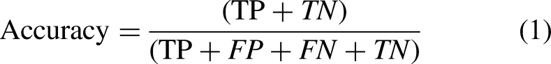

$$\mathrm{Accuracy}=\frac{(\mathrm{TP}+TN)}{(\mathrm{TP}+FP+FN+TN)}$$

(1)

Precision is referred to as the proportion of accurately anticipated positive values to all positively expected values. The formula can be depicted as:

$$\mathrm{Precision}=\frac{\mathrm{TP}}{(\mathrm{TP}+\mathrm{FP})}$$

(2)

Recall is defined as the proportion between the total number of actual values and the properly anticipated positive value. The formula can be depicted as:

$$\mathrm{Recall}=\frac{\mathrm{TP}}{(\mathrm{TP}+\mathrm{FN})}$$

(3)

The F1-Score is the harmonic mean of the precision and recall scores for a classification issue. The formula is as follows:

$$\text{F1-Score}=\frac{(2\times \mathrm{Precision}\times \mathrm{Recall})}{(\mathrm{Precision}+Recall)}$$

(4)

Here TN, TP, FN, and FP refer to true negative, true positive, false negative, and false positive values, respectively. If it is positive in both actual and predicted class then it is called TP (True 44 Positives), if in the actual class, it is positive but in predicted class it is negative then it is called FN, if in actual class it is negative and in predicted class it is positive then it is called FP, if in actual class it is negative and in predicted class also it is negative then it is called TN. While the TP and TN values represent the correct prediction, and FP and FN values represent the incorrect prediction of the class value. Therefore the lower the value of FN and FP the more reliable the model becomes.

CCE loss

In addition, the loss function was used in this study to evaluate how well the anticipated model performed. A CCE loss was used to train the model as well as to lower the cost of the model parameters. The value of the loss function is minimized by increasing the number of epochs. It is obtained using the depicted equation:

$$L(Y,\hat{Y})=-(\sum Y*\log (\hat{Y})+(1-Y)*\log \log (1-\hat{Y}))$$

(5)

where $Y$  = true label, $\hat{Y}$  = predicted labels & $L(Y,\hat{Y})$  = loss function.

Normalization of confusion matrix

Normalization of the confusion matrix is accomplished to compute and represent all the samples of each category on a scale of 1.00. The precision values are determined by adding the sums of the columns for each value or sample that is allocated to a certain class, and, then dividing the diagonal values by these sums. The diagonal values of the matrix represent the recall or sensitivity values. These values can be obtained using the following formula: 6.

$${\mathrm{Recall}}_{\mathrm{A}}={\mathrm{Sensitivity}}_{\mathrm{A}}=\frac{{\mathrm{TP}}_{\mathrm{A}}}{({\mathrm{TP}}_{\mathrm{A}}+E_{\mathrm{A}\mathrm{B}}+E_{\mathrm{A}\mathrm{C}}+E_{\mathrm{AD}})}$$

(6)

where diagonal values such as ${\mathrm{TP}}_{\mathrm{A}},{\mathrm{TP}}_{\mathrm{B}}$ , and so on represent TPs for the corresponding classes. The off-diagonal values of the normalized matrix are also calculated. For instance, the following equation may be used to get the value of the row “A” $\times$ column “B” cell.

$$\mathrm{AB}=\frac{E_{\mathrm{AB}}}{({\mathrm{TP}}_{\mathrm{A}}+E_{{\mathrm{A}}_{\mathrm{B}}}+E_{{\mathrm{A}}_{\mathrm{C}}}+E_{{\mathrm{A}}_{\mathrm{D}}})}$$

(7)

where $E_{\mathrm{BA}},E_{\mathrm{AC}}$ were referred to as the error values.

Area under the receiver operating characteristic curve (AUC-ROC) curve

Graphs that display the TP rate and FP rate of classifiers are known as AUC-ROC curves. It shows the AUC-ROC curve. We utilized the ROC curve in the binary class dataset to evaluate the performance. Usually, it plots the true positive rate (TPR) and false positive rate (FPR) on the $Y$ and $X$ axes, respectively. Since the range of both TPR and FPR is 0 to 1, the area remains between 0 and 1. The greater the AUC value the higher the performance.

Standard deviation (SD)

SD, a statistic that captures how much the data values deviate from the mean, is a frequently used method to quantify data spread. This is obtained by computing the square root of the variance, or the average of the squared deviations between each data value and the mean. When the SD is low, it indicates that the data values are near the mean; when it is high, it indicates that the data values are dispersed over a large range. The larger deviation also represents a larger bias or error. We computed the SD for model evaluation for both two-class and multi-class data.

Results analysis and discussion

As said previously this research explored two MRI brain tumor datasets for six deep learning frameworks. First, we launched the experiment on a small dataset containing only two types: “Yes” and “No.” After achieving remarkable accuracy in the small dataset, we relaunched the experiment on a big dataset containing three tumor classes. The outcome of these models according to the implemented methodology is analyzed for both datasets. The parameters of the models are trained and optimized taking batch size 13 on 70 epochs. To test the model’s gradient values in a small and big amount of data the experiment is launched using two widely used optimizers: Adam and AdaMax. Adam is selected as it functions well with a variety of paradigms, reduces memory requirements, and is easy to implement. Furthermore, it adjusts the learning rate for each weight of the neural network by estimating the first and second moments of the gradient. AdaMax is a variant of Adam that employs the L-infinity norm of the gradients rather than the second moment of the gradients. It is selected as it can handle the vanishing-gradient and exploding-gradient problems and also provide faster convergence. Besides AdaMax performs well in case of extremely sparse gradients.

Dataset-1 (two class)

We split the small dataset by taking 85% of the samples for training purposes, while the remaining 15% for testing. To keep the pdf smaller, we provided the loss, accuracy graph, and confusion matrix before and after normalization only for MobileNetV2 architecture. We launched two experiments in this dataset for the effective evaluation of the results.

Experiment 1

We perform classification by splitting the dataset. The classification result of each class is then evaluated using performance metrics precision, recall, F1-score, and accuracy for both optimizers.

Adam: To demonstrate how effectively the models worked, the models’ actual versus validation loss and accuracy are plotted through graphs. Since Adam adapts the learning rate easily, it makes computation time faster and requires fewer tuning parameters. The prediction outcomes in the corresponding classes using the Adam optimizer are shown in Figure 6 only for MobileNetV2 architecture. It shows that the FP and FN values are reduced to zero since the model can predict the actual number of data for the respective classes. Besides we see from the graph that the initial training and validation loss was too high. It decreases slowly and reduces to 0.011 while the training and validation accuracy increase to 1.0 after 20 epochs. According to Table 5 for Adam optimizer, we see that the actual prediction of the class Yes, No of all the models obtained is 100. The precision, recall, and F1-score values for each model are depicted in Table 6. From the table, we find that our models performed smoothly achieving the precision, recall, and F1-score value of 1.00 using the Adam optimizer.

Figure 6.

Performance results of MobileNetV2 using Adam optimizer for the two-class dataset: (a) actual versus validation loss; (b) actual versus validation accuracy; (c) confusion matrix before normalization; and (d) confusion matrix after normalization.

Table 5.

True prediction value of the classes obtained through the confusion matrix in the two-class dataset without cross-validation.

	Adam		AdaMax
Transfer learning (TL) model	Yes	No	Yes	No
VGG16	100%	100%	100%	100%
EfficientNetB3	100%	100%	100%	100%
DenseNet201	100%	100%	100%	100%
InceptionV3	100%	100%	100%	100%
ResNet50	100%	100%	100%	100%
MobileNetV2	100%	100%	100%	100%
Average	100%	100%	100%	100%

Table 6.

Performance analysis of the models using optimizer Adam on two-class datasets without cross-validation.

Models	Tumor class	Precission	Recall	F1-score
VGG16	Yes	1.00	1.00	1.00
	No	1.00	1.00	1.00
	Average	1.00	1.00	1.00
EfficientNetB3	Yes	1.00	1.00	1.00
	No	1.00	1.00	1.00
	Average	1.00	1.00	1.00
DenseNet201	Yes	1.00	1.00	1.00
	No	1.00	1.00	1.00
	Average	1.00	1.00	1.00
InceptionV3	Yes	1.00	1.00	1.00
	No	1.00	1.00	1.00
	Average	1.00	1.00	1.00
MobileNetV2	Yes	1.00	1.00	1.00
	No	1.00	1.00	1.00
	Average	1.00	1.00	1.00
ResNet50	Yes	1.00	1.00	1.00
	No	1.00	1.00	1.00
	Average	1.00	1.00	1.00

AdaMax: Further to examine the effectiveness of the AdaMax optimizer, we relaunched the experiments using AdaMax. The use of the L-infinity norm in AdaMax makes it more stable than Adam. We show the actual versus validation loss and accuracy and prediction of classes for the architecture in Figure 7 using AdaMax optimizer. From the normalized confusion matrix, we see that the TP value of each class is 1 which shows 100% prediction of the actual class values. Besides the graph depicts that both the training and validation loss is minimized to 0.012 and the accuracy is increased to 1. The performance scores for the AdaMax optimizer are also demonstrated in Table 7. According to Table 5 for AdaMax optimizer, we see that the actual prediction of the class Yes, No of all the models obtained is 100. Using AdaMax, we obtain the same precision, recall, and F1-score value as we got using Adam. The comparison of training and testing accuracy using these two optimizers is depicted in Table 8. From the table, we conclude that our proposed framework can predict brain tumors with 100% test accuracy in all the implemented TL algorithms for both Adam and AdaMax optimizers in this dataset.

Figure 7.

Performance results of MobileNetV2 using AdaMax optimizer for the two-class dataset: (a) actual versus validation loss; (b) actual versus validation accuracy; (c) confusion matrix before normalization; and (d) confusion matrix after normalization.

Table 7.

Performance analysis of the models using optimizer AdaMax on two-class datasets.

Models	Tumor class	Precission	Recall	F1-score
VGG16	Yes	1.00	1.00	1.00
	No	1.00	1.00	1.00
	Average	1.00	1.00	1.00
EfficientNetB3	Yes	1.00	1.00	1.00
	No	1.00	1.00	1.00
	Average	1.00	1.00	1.00
DenseNet201	Yes	1.00	1.00	1.00
	No	1.00	1.00	1.00
	Average	1.00	1.00	1.00
InceptionV3	Yes	1.00	1.00	1.00
	No	1.00	1.00	1.00
	Average	1.00	1.00	1.00
MobileNetV2	Yes	1.00	1.00	1.00
	No	1.00	1.00	1.00
	Average	1.00	1.00	1.00
ResNet50	Yes	1.00	1.00	1.00
	No	1.00	1.00	1.00
	Average	1.00	1.00	1.00

Table 8.

Accuracy of the transfer learning models on two-class datasets using our proposed methodology.

Transfer learning	Adam		AdaMax
models	Training accuracy (%)	Testing accuracy (%)	Training accuracy (%)	Testing accuracy (%)
VGG16	100	100	100	100
EfficientNetB3	100	100	100	100
DenseNet201	100	100	100	100
InceptionV3	100	100	100	100
ResNet50	100	100	100	100
MobileNetV2	100	100	100	100

As for both optimizers, the training and testing accuracy of all the models are recorded to 100, we launched another experiment in this dataset to validate the model performance.

Experiment 2

We launched this experiment implementing a five-fold CV approach along with various performance metrics precision, recall, F1-score, accuracy, SD, and AUC-ROC curve using AdaMax optimizers. The value of these metrics for each fold is listed through Tables 9 and 10 of all the model. We computed the average of the results obtained in all the test sets for all the metrics.

Table 9.

Performance analysis of the models using optimizer AdaMax on two-class datasets after cross-validation.

Models	Folds	Tumor	Precission	Recall	F1-score	Accuracy	ROC		Prediction
		Class				(%)	value (%)	SD	time (s)
VGG16	Fold1	Yes	1.00	1.00	0.99	99.87	100	0.119	8
		No	1.00	0.99	1.00
	Fold2	Yes	0.99	1.00	0.99	99.91	100	0.116	9
		No	1.00	0.99	1.00
	Fold3	Yes	0.99	1.00	1.00	99.83	100	0.120	7
		No	1.00	0.98	0.99
	Fold4	Yes	0.99	1.00	1.00	99.95	100	0.115	6
		No	0.99	1.00	1.00
	Fold5	Yes	0.99	0.99	0.99	99.80	100	0.120	7
		No	1.00	0.98	0.99
	Average	Yes	0.992	0.998	0.994	99.872	100	0.118	7.4
		No	0.998	0.98	0.996
EfficientNetB3	Fold1	Yes	0.99	1.00	1.00	99.95	100	0.111	9
		No	0.99	0.99	1.00
	Fold2	Yes	1.00	1.00	0.99	99.92	100	0.115	10
		No	0.99	1.00	1.00
	Fold3	Yes	1.00	1.00	1.00	99.96	100	0.108	8
		No	1.00	1.00	0.99
	Fold4	Yes	0.99	0.99	1.00	99.93	100	0.114	9
		No	0.99	1.00	0.99
	Fold5	Yes	1.00	1.00	1.00	99.98	100	0.105	8
		No	1.00	0.99	1.00
	Average	Yes	0.996	0.998	0.998	99.948	100	0.111	8.8
		No	0.994	0.996	0.996
DenseNet201	Fold1	Yes	0.99	1.00	1.00	99.94	100	0.114	10
		No	1.00	1.00	1.00
	Fold2	Yes	1.00	0.99	1.00	99.96	100	0.112	11
		No	1.00	1.00	0.99
	Fold3	Yes	1.00	0.99	0.99	99.93	100	0.115	9
		No	0.99	1.00	0.99
	Fold4	Yes	1.00	1.00	0.99	99.986	100	0.109	9
		No	1.00	1.00	1.00
	Fold5	Yes	1.00	0.99	0.99	99.918	100	0.117	10
		No	0.99	0.99	0.99
	Average	Yes	0.998	0.994	0.994	99.943	100	0.113	9.8
		No	0.996	0.998	0.994
InceptionV3	Fold1	Yes	1.00	1.00	0.99	99.96	100	0.110	6
		No	1.00	1.00	1.00
	Fold2	Yes	1.00	1.00	0.99	99.93	100	0.112	6
		No	0.99	1.00	1.00
	Fold3	Yes	0.99	1.00	1.00	99.97	100	0.108	5
		No	1.00	0.99	0.99
	Fold4	Yes	1.00	0.99	1.00	99.91	100	0.115	4
		No	0.99	0.99	1.00
	Fold5	Yes	1.00	1.00	1.00	99.996	100	0.103	5
		No	1.00	1.00	1.00
	Average	Yes	0.998	0.998	0.996	99.95	100	0.110	5.2
		No	0.996	0.996	0.998

ROC: receiver operating characteristic; SD: standard deviation.

Table 10.

Performance analysis of the models using optimizer AdaMax on two-class datasets after cross-validation.

Folds	Models	Tumor Class	Precission	Recall	F1-score	Accuracy (%)	ROC value (%)	SD	Run time (s)
MobileNetV2	Fold1	Yes	1.00	1.00	1.00	99.97	100	0.104	5
		No	1.00	0.99	1.00
	Fold2	Yes	1.00	1.00	1.00	99.98	100	0.103	4
		No	1.00	1.00	0.99
	Fold3	Yes	1.00	0.99	1.00	99.94	100	0.109	5
		No	o.99	1.00	1.00
	Fold4	Yes	0.99	0.99	1.00	99.95	100	0.107	4
		No	1.00	1.00	0.99
	Fold5	Yes	1.00	1.00	1.00	99.998	100	0.100	4
		No	1.00	1.00	1.00
	Average	Yes	0.998	0.996	1.00	99.966	100	0.105	4.4
		No	0.998	0.998	0.996
ResNet50	Fold1	Yes	1.00	0.99	1.00	99.92	100	0.116	9
		No	0.99	1.00	1.00
	Fold2	Yes	0.99	1.00	0.99	99.94	100	0.115	8
		No	1.00	1.00	0.99
	Fold3	Yes	1.00	0.99	1.00	99.91	100	0.116	8
		No	0.99	1.00	0.99
	Fold4	Yes	1.00	1.00	0.99	99.96	100	0.113	7
		No	1.00	1.00	1.00
	Fold5	Yes	0.99	0.99	1.00	99.90	100	0.118	7
		No	1.00	0.99	0.99
	Average	Yes	0.996	0.994	0.996	99.88	100	0.116	7.8
		No	0.996	0.998	0.994

ROC: receiver operating characteristic; SD: standard deviation.

After CV, the VGG16 model achieved the highest accuracy of 99.95% in Fold4 with an SD of 0.115. The model achieved an average accuracy of 99.87% and an average SD of 0.120. EfficientNetB3 model achieved the highest accuracy of 99.98 in Fold5 with an SD of 0.105. The model achieved an average accuracy of 99.95% and an average SD of 0.111. DenseNet201 model achieved the highest accuracy of 99.986 in Fold4 with an SD of 0.109. The model achieved an average accuracy of 99.943 and an average SD of 0.113. InceptionV3 model achieved the highest accuracy of 99.996% in Fold5 with an SD of 0.103. The model achieved an average accuracy of 99.95 and an average SD of 0.110. MobileNetV2 model achieved the highest accuracy of 99.998 in Fold5 with an SD of 0.100. The model achieved an average accuracy of 99.96% and an average SD of 0.105. ResNet50 model achieved the highest accuracy of 99.96 in Fold4 with an SD of 0.109. The model achieved an average accuracy of 99.943% and an average SD of 0.113. As the result achieved effective outcome in all the parameters there is no issue of potential bias.

Dataset-2 (Four Class)

We justified the performance obtained in the two class 253 image dataset utilizing another four-class dataset. We split this dataset by taking 80% of the samples for training purposes, while the remaining 20% for testing. The classification of tumor classes is carried out for all the selected models. The result is evaluated through precision, recall, F1-score, accuracy, and SD. The model can classify glioma, meningioma, pituitary tumor tissues, and normal brain tissues more accurately.

Adam: Using Adam optimizer the training and validation loss and accuracy along with the prediction of the actual class label for the MobileNetV2 architecture is depicted in Figure 8. We can easily understand the number of actual and false predictions of each class for each model from the normalized confusion matrix. As depicted in the graph, in the first epoch, the loss was high while accuracy was low. In the first 20 epochs, the training loss is minimized to almost 0.0 and the accuracy has increased. The validation loss is also minimized to 0.1. Besides, we added the prediction of each class through the normalized confusion matrix in Tables 11. On an average 98.3% of the meningioma class and without tumor images has been truly predicted. The Glioma class contains more misclassified images than others. Furthermore, we can see the precision, recall, and F1-score values for the corresponding class of the models in Table 12. The models achieved an average 97% precision, recall, and F1-score value in all the classes. According to Tables 13 and 14, the highest accuracy obtained is 98.20% for MobileNetV2 architecture with a small deviation of 0.120.

Figure 8.

Performance results of MobileNetV2 using Adam optimizer for the four-class dataset: (a) actual versus validation loss; (b) actual versus validation accuracy; (c) confusion matrix before normalization; and (d) confusion matrix after normalization.

Table 11.

True prediction value of the classes obtained through the confusion matrix in the four-class dataset.

	Adam				AdaMax
TL model	Glioma	Meningioma	Pituitary	No_tumor	Glioma	Meningioma	Pituitary	No_tumor
VGG16	94%	96%	98%	97%	94%	96%	98%	96%
EfficientNetB3	96%	99%	95%	100%	97%	99%	95%	100%
DenseNet201	94%	100%	95%	99%	95%	100%	96%	98%
InceptionV3	95%	100%	95%	99%	94%	100%	97%	90%
ResNet50	96%	95%	99%	99%	96%	99%	100%	97%
MobileNetV2	97%	100%	97%	99%	96%	100%	97%	99%
Average	95.3%	98.3%	96.5%	98.3%	95.3%	99%	97.2%	98.2%

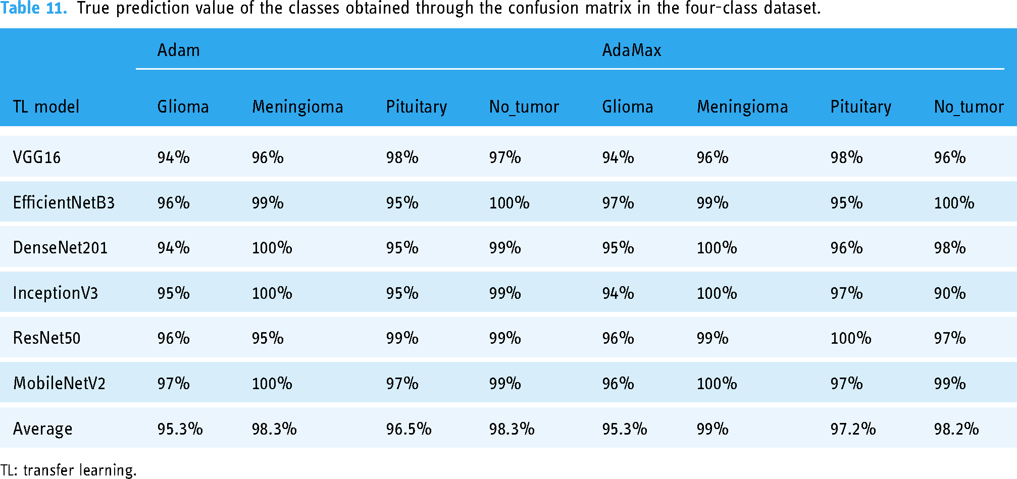
TL: transfer learning.

Table 12.

Performance analysis of the models for four classes using optimizer Adam.

Models	Tumor class	Precission	Recall	F1-score
VGG16	Glioma	0.97	0.94	0.95
	Meningioma	0.95	0.96	0.96
	No_tumor	0.97	0.97	0.97
	Pituitary	0.99	0.98	0.98
	Average	0.97	0.9625	0.96
EfficientNetB3	Glioma	0.96	0.96	0.96
	Meningioma	0.99	0.99	0.99
	No_tumor	0.97	1.00	0.99
	Pituitary	0.97	0.95	0.96
	Average	0.9725	0.975	0.975
DenseNet201	Glioma	0.97	0.97	0.96
	Meningioma	0.96	0.96	0.98
	No_tumor	0.98	0.96	0.97
	Pituitary	0.97	1.00	0.98
	Average	0.97	0.97	0.98
InceptionV3	Glioma	0.96	0.95	0.96
	Meningioma	0.98	1.00	0.99
	No_tumor	0.97	0.99	0.98
	Pituitary	0.98	0.95	0.96
	Average	0.9725	0.9725	0.9725
MobileNetV2	Glioma	0.98	0.97	0.98
	Meningioma	1.00	1.00	1.00
	No_tumor	0.97	0.99	0.98
	Pituitary	0.98	0.97	0.98
	Average	0.98	0.9825	0.98
ResNet50	Glioma	0.99	0.96	0.97
	Meningioma	0.97	0.95	0.96
	No_tumor	0.97	0.99	0.98
	Pituitary	0.96	0.99	0.97
	Average	0.9725	0.9725	0.97

Table 13.

Performance analysis of the models for four classes using optimizer AdaMax.

Models	Tumor class	Precission	Recall	F1-score
VGG16	Glioma	0.95	0.95	0.96
	Meningioma	0.95	0.97	0.96
	No_tumor	0.97	0.97	0.97
	Pituitary	0.98	0.98	0.98
	Average	0.96	0.97	0.97
EfficientNetB3	Glioma	0.96	0.97	0.97
	Meningioma	0.98	0.99	0.99
	No_tumor	0.97	1.00	0.99
	Pituitary	0.98	0.95	0.97
	Average	0.9725	0.9775	0.98
DenseNet201	Glioma	0.98	0.95	0.96
	Meningioma	0.98	1.00	0.99
	No_tumor	0.97	0.98	0.97
	Pituitary	0.96	0.96	0.96
	Average	0.97	0.9725	0.97
InceptionV3	Glioma	0.98	0.94	0.96
	Meningioma	0.98	1.00	0.99
	No_tumor	0.94	0.99	0.96
	Pituitary	0.98	0.97	0.97
	Average	0.97	0.975	0.97
MobileNetV2	Glioma	0.98	0.96	0.97
	Meningioma	1.00	1.00	1.00
	No_tumor	0.95	0.99	0.96
	Pituitary	0.99	0.97	0.98
	Average	0.98	0.98	0.98
ResNet50	Glioma	1.00	0.93	0.96
	Meningioma	0.96	1.00	0.97
	No_tumor	0.99	0.99	0.99
	Pituitary	1.00	0.99	0.99
	Average	0.97	0.97	0.97

Table 14.

Accuracy and standard deviation (SD) of the transfer learning models on four class datasets using our proposed methodology.

Transfer learning	Adam			AdaMax
models	Training	Testing	SD	Training	Testing	SD
	accuracy (%)	accuracy (%)		accuracy (%)	accuracy (%)
VGG16	99.96	96.34	0.145	99.923	96.21	0.143
EfficientNetB3	100	97.94	0.133	100	97.98	0.130
DenseNet201	100	97.23	0.158	100	97.70	0.151
InceptionV3	99.94	97.90	0.129	100	97.90	0.132
ResNet50	100	97.77	0.183	100	96.85	0.174
MobileNetV2	100	98.20	0.120	100	98.16	0.121

AdaMax: The loss, accuracy graph, and the normalized results of the confusion matrix using AdaMax optimizer are shown in Figure 9. The actual prediction of the classes using AdaMax is recorded in Table 11. AdaMax has increased the average true positive value for meningioma, pituitary, and no_tumor classes. The most misclassified class is gloma. On average 99% of the meningioma class, 98.2% of the no_tumor class, 97.2% of the pituitary class, and 95.3% of the glioma class images are truly predicted using AdaMax. Some samples of misclassified images are shown in Figure 10. The performance scores of the models are demonstrated in Table 13. The average precision, recall, and F1-score value of each class is between 0.96 and 0.98. Table 14 displays a comparison of training and testing accuracy obtained through Adam and AdaMax optimizer on this dataset. The accuracy of ResNet50 is decreased in AdaMax while the accuracy of DenseNet201 has increased. Comparing the testing accuracy we can say that MobileNetV2 architecture has the highest performance with an accuracy of 98.16% and an SD of 0.121 while VGG16 has the lowest accuracy of 96.21% and an SD of 0.143 using our proposed framework. In addition, we can train the models using the presented methodology with 100% accuracy.

Figure 9.

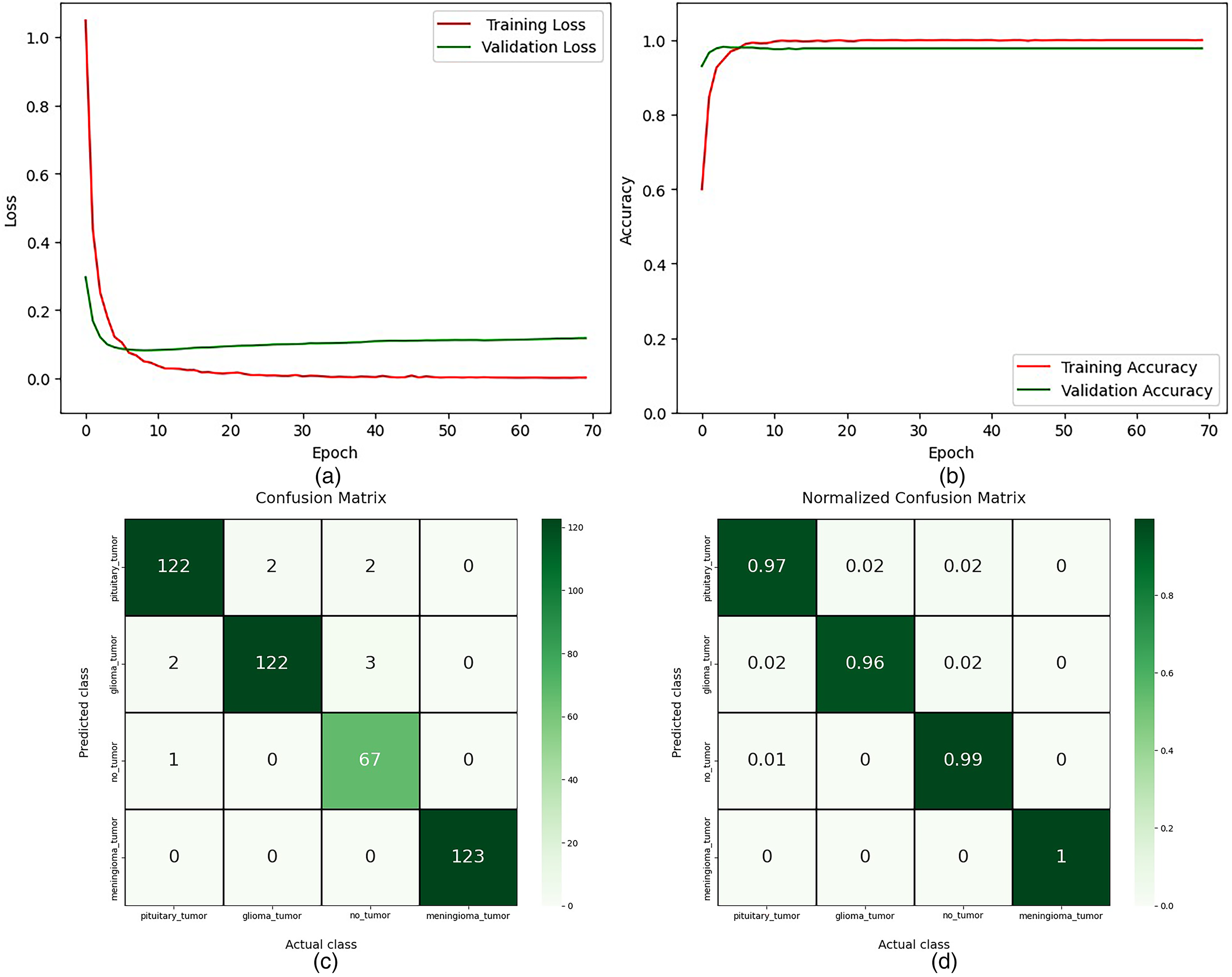
Performance results of MobileNetV2 using AdaMax optimizer for the four-class dataset: (a) actual versus validation loss; (b) actual versus validation accuracy; (c) confusion matrix before normalization; and (d) confusion matrix after normalization.

Figure 10.

Some samples of misclassified images.

Discussion

To get a stable accuracy, we observe the result by increasing the number of epochs from 50 to 70. In experiment one, our proposed model achieves 100% testing accuracy on the two-class dataset. In experiment two, our proposed framework obtained 99.99% testing accuracy with ROC 100 utilizing the CV method on the two-class dataset. Furthermore, in the four-class dataset, our model achieved 98.20% accuracy. Our proposed framework has reduced the overfitting issues of the model. Tables 8 and 14 show that the performance results for Adam and AdaMax optimizers are quite similar. However, as indicated in Table 15, AdaMax demonstrates faster computational performance compared to Adam, reducing the time per epoch except for VGG16 and ResNet50. MobileNetV2, with the fewest parameters, exhibits the lowest execution time and highest accuracy, while InceptionV3 follows as the second fastest model with high accuracy. In contrast, DenseNet201, EfficientNetB3, and ResNet50 require significantly more computational time, but these models also provide high accuracy values. VGG16, despite its popularity, shows lower effectiveness in precision, recall, F1-score, and overall accuracy compared to other models. The number of total parameters, trainable parameters, and non-trainable parameters in each model remains constant regardless of the optimizer or dataset used. However, the execution time of different models is also influenced by the number of layers and parameters.

Table 15.

Parameters details and execution time of the models on both datasets using our proposed methodology.

	Run time (s)
				Dataset-1		Dataset-2
	Total	Non-trainable	Total	Adam	AdaMax	Adam	AdaMax
TL model	parameters	parameters	layers
ResNet50	23,710,896	53,120	50	180	200	500	520
InceptionV3	21,925,968	34,432	159	130	93	350	260
DenseNet201	18,437,488	229,056	201	290	248	1000	966
VGG16	14,745,712	0	16	145	138	632	490
EfficientNetB3	10,875,999	87,303	234	240	208	523	480
MobileNetV2	2,335,088	34,112	88	80	80	230	200

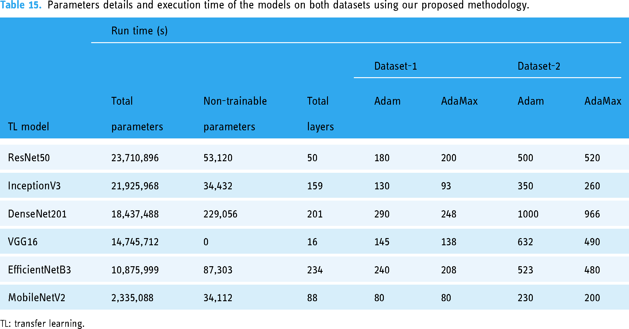
TL: transfer learning.

Comparison with the state-of-the-art methods

To address the detection and classification of brain tumors, numerous researchers around the world are working incredibly hard. Several datasets have been created using the clinical brain MRI reports of a lot of patients and various methodologies emerged of extreme research in this field. A comparison is carried out to demonstrate the efficacy of our experimented framework with other state-of-the-art methods considering both the 253 image dataset and the 3264 image dataset.

The experimented results of our proposed methodology for the corresponding study on the small dataset are illustrated in Table 16 along with the other state-of-the-art models. As listed in the table, in the small binary class dataset, our implemented framework appeared with excellently higher performance. As mentioned earlier, we achieved a test accuracy of 100% in all the selected models with the precision, recall, F1-score value 1.00 in each class in experiment one according to Tables 6 to 8. Our model can predict the actual number of each class with 100% accuracy as shown in Table 5. Besides the execution time of our model is also very small compared to others as shown in Table 15. Another experiment on the small dataset also achieved outstanding accuracy, ROC value, precision, recall, and F1-score value with small deviation for each fold of CV as shown in Tables 9 and 10. However, Hassan et al. ³⁸ classified brain tumors utilizing VGG-16, ResNet-50, and Inception-v3 architecture using this 253 BT dataset with accuracy 96%, 89%, and 75% accuracy at VGG-16, ResNet-50, and Inception-V3, respectively. Their model obtained very poor accuracy while lacking other performance metrics for result analysis. Furthermore, they did not perform fine-tuning of the parameters. Arbane et al. ³⁵ implemented three TL architectures, namely ResNet, Xception, and MobilNet-V2 to categorize brain MRI. This attained the best results with 98.24% and 98.42% in terms of accuracy and F1-score, respectively. To create tumor boundary they applied the OpenCV method. However, their model is computationally complex to build and lower accuracy compared to our model. An automated hybrid system for classifying brain tumors is presented by Kang et al. ³⁰ To ensemble three top features they utilized several pre-trained deep learning models for feature extracting with various ML classifiers. The study reported 92.16% accuracy on the BT-small-2c dataset. Except for accuracy, they did not measure any other performance score and also did not analyze the computation time of their hybrid model.

Table 16.

Performance results in comparison among the suggested model and the other previous state-of-art works based on four class categories using 253 magnetic resonance (MR) image dataset.

Study (year)	Architecture	Dataset	Accuracy (%)
Hassan et al. (2020)	VGG-16,	253 MR images	96
	ResNet-50,		89
	Inception-v3		75
Mohamed Arbane et al. (2021)	ResNet, Xception	253 MR images	98.24
	and MobilNet-V2
Jaeyong Kang et al. (2021)	VGG16,	253 MR images	92.09
	ResNet50		95.15
	DenseNet169		95.70
	InceptionV3		95.81
	MobileNetV2		94.70
Proposed Methodology	VGG16,	253 MR images	100
	EfficientNetB3		100
(Without cross-validation)	ResNet50		100
	DenseNet201		100
	InceptionV3		100
	MobileNetV2		100
Proposed Methodology	VGG16,	253 MR images	99.87
	EfficientNetB3		99.95
(After cross-validation)	ResNet50		99.88
	DenseNet201		99.94
	InceptionV3		99.95
	MobileNetV2		99.96

The experimented results for the corresponding study on the big dataset are illustrated in Table 17 along with the other state-of-the-art models. The highest accuracy obtained in our experiment is 98.20% with a little deviation of 0.120. The precision, recall, and F1-score values are also higher in this dataset. Besides our model has low computational time thus low computation complexity compared to the existing studies. While the accuracy of the existing model is not more than 90%. Their accuracy is comparatively very low. However, our models performed smoothly on both datasets for all the selected architectures with greater accuracy. Sunanda Das et al. ²⁷ developed a CNN model for the classification of brain tumors in T1-weighted contrast-enhanced MRI images; a dataset of 3064 photos of three different forms of brain tumors (glioma, meningioma, and pituitary). They used a Gaussian filter, and histogram equalization to preprocess the input data and three dropout layers in the classification model with a dropout rate of 25%, 40%, and 30%. Though dropout reduces overfitting, inappropriate dropout rates decrease the strength of the neural network. However, they gained a testing accuracy of 94.39%. Their testing loss is high. Parnian et al. ²⁹ developed Capsule Networks (CapsNets) to overcome the shortcomings in CNN to fully utilize spatial relations. The suggested improved CapsNet architecture incorporates additional inputs from the tumor coarse borders into its pipeline to sharpen the CapsNet’s focus. The model handled transformations in a “Routing by Agreement” process instead of a pooling layer, during which lower-level capsules forecast how their higher-level parents will behave. However, this method is incapable of interpreting the features of brain tumors efficiently. They do not perform any pre-processing technique. Their model does not obtain a higher prediction outcome, on the contrary, model computation is complex. The accuracy of this approach is 90.89%. Utilizing a hybrid system for classifying brain tumors, Kang et al. ³⁰ achieved 93.72% accuracy on the BT-large-4c dataset. The model is not reliable. Their prediction outcome is also lower than us. Besides except accuracy, they did not measure any other performance score and also did not analyze the computation time of their hybrid model.

Table 17.

Performance results in comparison among the suggested model and the other previous state-of-the-art works based on four class categories using the 3064 MR image dataset.

Study (year)	Architecture	Dataset	Accuracy (%)
Sunanda Das et al. (2019)	CNN	3064 MR images	94.39
Parnian Afshar et al. (2019)	Modified CNN,	3064 MR images	88.33
	CapsNet		90.89
Jaeyong Kang et al. (2021)	VGG16,	3064 MR images	81.73
	ResNet50		82.73
	DenseNet169		84.87
	InceptionV3		81.23
	MobileNetV2		84.40
Proposed Methodology	VGG16,	3264 MR images	96.34
	EfficientNetB3		97.98
	ResNet50		97.77
	DenseNet201		97.70
	InceptionV3		97.90
	MobileNetV2		98.20

CNN: convolutional neural network; MR: magnetic resonance.

Practical implications and limitations

Although our proposed models demonstrated superior performance, it is essential to discuss their practical implications. Integrating these models into clinical workflows could potentially enhance the accuracy and efficiency of brain tumor diagnosis. However, challenges such as the need for robust validation in diverse clinical settings, potential biases in the datasets, and the limitations of the study should be acknowledged. Further validation and testing in real-world scenarios are necessary to confirm the generalizability of the models.

Ethical considerations of artificial intelligence (AI) models in clinical environments

To address ethical considerations in implementing AI models in clinical environments:

Patient confidentiality: Ensure robust data protection, including encryption, anonymization, and compliance with regulations such as Health Insurance Portability and Accountability Act and General Data Protection Regulation to safeguard patient information.

Algorithmic bias: Mitigate bias by using diverse, representative datasets and regularly auditing the model to ensure fair treatment across demographic groups.

Transparency and accountability: Provide clear explanations of AI decisions, ensuring the model serves as a support tool, with healthcare providers retaining final responsibility for diagnoses.

Continuous monitoring: Regularly monitor and update AI models to maintain accuracy and relevance, ensuring they adapt to evolving medical knowledge and patient needs.

Addressing these concerns promotes responsible AI use in healthcare, prioritizing patient safety and fairness.

Conclusions

This experiment successfully developed an efficient and fine-tuned deep neural network architecture utilizing pre-trained models for the detection and classification of brain tumors. From data collection to feature extraction, the experiment employed effective preprocessing techniques, data augmentation, and fine-tuning of parameters, leading to the reconstruction of models and the observation of robust outcomes. Iterative optimization of various parameters resulted in stable and high prediction accuracy. Regularization and the addition of extended layers significantly enhanced prediction accuracy while reducing model overfitting. In addition, implementation of CV with several evaluation metrics makes the model computationally effective.

Among the six implemented models, MobileNetV2 stood out with the lowest execution time and highest accuracy, whereas VGG16 faced challenges and achieved the lowest accuracy. The comparison between the Adam and AdaMax optimizers showed consistent results, with AdaMax offering faster computation. For the small dataset, all models achieved 100% accuracy without CV for both training and testing. After performing CV, the models generate an average accuracy of 99.96% with higher precision, recall, F1-score, and ROC value demonstrating the effectiveness of our framework. On the larger dataset, the models maintained strong performance, with the highest testing accuracy reaching 98.20% and training accuracy reaching 100%.

Our experiment shows that the proposed framework is robust, reliable, and capable of supporting medical professionals in the timely and accurate diagnosis of brain tumors. However, real-time implementation and integration into clinical workflows would require further validation in diverse clinical settings.

Future work

Future research will focus on:

Larger and diverse datasets: Expanding the framework by utilizing larger and more varied MRI datasets to improve generalizability.

Multi-modal integration: Enhancing diagnostic accuracy by integrating other medical imaging modalities, such as CT or PET scans, and combining them with genetic and clinical data.

Data scarcity and imbalance: Addressing data scarcity and class imbalance through techniques such as synthetic data generation, TL, and advanced oversampling.

Advanced fine-tuning: Further optimizing models using hyperparameter tuning and training with larger datasets for more precise predictions.

These steps aim to enhance the framework’s real-world applicability and effectiveness in brain tumor diagnosis.