Melanoma identification and classification model based on fine-tuned convolutional neural network

Abstract

Background

Breakthroughs in skin cancer diagnostics have resulted from recent image recognition and Artificial Intelligence (AI) technology advancements. There has been growing recognition that skin cancer can be lethal to humans. For instance, melanoma is the most unpredictable and terrible form of skin cancer.

Materials and Methodology

This paper aims to support Internet of Medical Things (IoMT) applications by developing a robust image classification model for the early detection of melanoma, a deadly skin cancer. It presents a novel approach to melanoma detection using a Convolutional Neural Network (CNN)-based method that employs image classification techniques based on Deep Learning (DL). We analyze dermatoscopic images from publicly available datasets, including DermIS, DermQuest, DermIS&Quest, and ISIC2019. Our model applies convolutional and pooling layers to extract meaningful features, followed by fully connected layers for classification.

Results

The proposed CNN model achieves high accuracy demonstrates the model’s effectiveness in distinguishing between malignant and benign skin lesions. We developed deep features and used transfer learning to improve the categorization accuracy of medical images. Soft-max classification layer and support vector machine have been used to assess the classification performance of deep features. The proposed model’s efficacy is rigorously evaluated using benchmark datasets: DermIS, DermQuest, and ISIC2019, having 621, 1233, and 25000 images, respectively. Its performance is compared to current best practices showing an average of 5% improved detection accuracy in DermIS, 6% improvement in DermQuest, and 0.81% in ISIC2019 datasets.

Conclusion

Our study showcases the potential of CNN in melanoma detection, contributing to early diagnosis and improved patient outcomes. The developed model proves its capability to aid dermatologists in accurate decision-making, paving the way for enhanced skin cancer diagnosis.

Introduction

In recent decades, skin cancer has been among the most prevalent causes of death worldwide, contributing to the overall rise in cancer-related mortality rates. Countries with extreme weather patterns and long-term solar exposure are the known causes. ¹ Skin lesions may be benign or malignant, such as melanoma, pigmented benign keratosis, basal cell carcinoma, or squamous cell carcinoma.^2,3 Due to the great degree of similarities between various skin lesions, visual inspection remains difficult and may result in an incorrect diagnosis. Therefore, a highly efficient and well-trained professional is needed for manual diagnosis due to the high resemblance across lesions. ⁴ Melanoma, a skin cancer type, can be deadly without early detection. Much study continues to focus on developing more accurate methods of detecting melanoma at an early stage so that medical professionals can more accurately distinguish between the two. Traditional techniques were used to extract critical visual features based on color and texture in images, whereas contemporary technology takes cues from natural processes, such as Artificial Intelligence (AI) ⁵ and Deep Learning (DL), ⁶ e.g., Convolutional Neural Networks (CNNs). ⁷ Deep CNN (DCNN) learns systematically using a variety of inputs. Data scarcity, segmentation, pre-processing, and augmentation hamper the performance of existing computer-aided approaches for dermatological image classification. ⁸

The adoption of AI has significantly led to the early identification of melanoma. ⁹ Particularly, CNNs have demonstrated promising results in melanoma detection from images. ¹⁰ By adjusting the hyperparameters of CNNs, researchers have improved their accuracy and decreased the number of false positives in melanoma detection.^11–13 In addition, incorporating Internet of Things (IoT) or Internet of Medical Things (IoMT) ¹⁴ devices with CNNs has made it possible to diagnose melanoma non-invasively by capturing images of the skin lesion using a smartphone or other portable devices.^15,16 This integration has increased the accessibility of melanoma detection, particularly in remote or low-resource areas with limited access to healthcare facilities. CNNs can autonomously learn features from images and attain high classification accuracy.^17,18 However, it depends significantly on hyperparameters such as learning rate, sample size, and the number of layers to achieve optimal performance. The process of determining the optimal combination of hyperparameters for a given task is known as hyperparameter optimization. It is crucial in developing CNN-based melanoma detection systems with high accuracy and generalizability on unobserved data. ¹⁹

However, tuning the hyperparameters of a CNN is crucial for increasing the detection accuracy of melanomas. Finding the optimal hyperparameter values can substantially enhance the model’s precision and generalizability. The model may suffer from underfitting or overfitting if the hyperparameters are not appropriately tailored. ²⁰ The primary cause of underfitting is the oversimplified model that cannot represent the data’s complexity. It induces poor performance for the training and testing datasets. On the other hand, overfitting arises when a model is overly complex and suits the training data too closely, resulting in inadequate generalization to new, untrained data. Fine-tuning hyperparameters can prevent both issues and increase the model’s precision. Adjusting the learning rate, for instance, can help the model converge more quickly during training, while increasing the number of layers can enhance the model’s capacity to learn intricate features. This paper presents a comprehensive technical analysis of hyperparameter optimization for CNN-based melanoma detection. Through meticulous experimentation, we unearth the remarkable potential of hyperparameter tuning to refine and fundamentally elevate the prowess of CNN-based melanoma detection. Our revelations stand poised to reshape the landscape of medical imaging, driving the evolution of melanoma detection systems toward unparalleled accuracy and efficiency, all within the powerful framework of CNN technology. The paper contributions are summarized as follows:

Introducing a CNN-based method for melanoma detection that employs image classification techniques based on DL.

Investigating the efficacy of CNN hyperparameter fine-tuning in enhancing the detection accuracy of melanomas to aid dermatologists in providing an accurate and timely diagnosis.

The proposed model is augmented using mathematical modeling and formal description, which is further elaborated using mathematical examples.

Evaluating the proposed method on benchmark datasets and comparing the results to current best practices.

Review the most recent research on melanoma detection using DL techniques, including various approaches, datasets, and performance measures.

Improving accuracy, precision, recall, and F1-Score for the benchmark datasets.

This paper constitutes the following sections: The literature review is analyzed in the “Related work” section, followed by the background in the “Background” section. The Alexnet model is presented in the “AlexNet model” section, and the “Proposed architecture and model” section details the proposed architecture and model. The Experimentation and results are delineated in the “Experimentation and results” section, whereas the conclusion is in the “Conclusion and future work” section.

Related work

This section details various classification studies of skin cancer using machine learning models and their comprehensive analysis.

Promising findings for employing Support Vector Machines (SVMs) to predict melanoma skin cancer are discussed by Lingaraj et al. ²¹ However, the results cannot be applied to a broader population due to the study’s limited sample size and absence of external validation. Another possible drawback is that SVM models are not easily interpretable, and in clinical settings, it is essential to consider the model’s specificity and false-positive rate. Machine learning models’ clinical value and cost-effectiveness in clinical settings should be evaluated. Future research should confirm the model’s performance on external datasets and produce more interpretable models. Using DL models, the authors ²² investigated the influence of several pre-processing methods on the classification accuracy of skin lesion photographs. They discovered that pre-processing methods might considerably increase the classification accuracy of photos of skin lesions, with CLAHE producing the overall best outcomes. The scientists also offer insights into the processes underpinning the enhanced performance, which will help guide future studies on the classification of skin lesions. Overall, the study significantly adds to skin lesion classification by highlighting the value of pre-processing approaches and outlining the best ones. The results significantly enhance the precision and dependability of DL-based automated skin lesion detection. The study uses a single dataset constraint, and further investigation is needed to see whether the results can be applied to other populations and other datasets. Liang and Wu ²³ evaluated the effectiveness of decision trees and neural network algorithms in identifying skin cancer from dermoscopy images. The neural network algorithm outperformed the decision tree algorithm in terms of sensitivity, but both the neural network and decision tree algorithms demonstrated high accuracy in detecting skin cancer. However, it did not consider the algorithms’ specificity, which is crucial in clinical practice to prevent false positives and pointless biopsies. The study only used a small dataset, which may limit how broadly the results can be applied to other populations and datasets. The authors did not address the number of malignant and benign cases being imbalanced, variations in image quality and lighting conditions, or other potential biases in the dataset. These biases may impact the effectiveness and generalizability of the algorithms.

To increase the precision of skin cancer classification, Ashraf et al. ²⁴ proposed a CNN-based architecture that considered global and local skin lesion attributes. The article offers a promising advancement in DL-based skin cancer classification. However, the suggested model may increase the efficacy and accuracy of a skin cancer diagnosis while lowering the demand for invasive biopsies. In addition, The number of convolutional layers (CLs), filters, pooling operations, and how the hyperparameters were chosen for the CNN architecture should have been explained. Hyperparameter tuning is crucial to maximize the capabilities of the CNN architecture and guarantee its transferability to other datasets. The study only used a small sample of images of skin lesions, which may have limited generalized results. To identify skin cancer, Ashraf et al. ²⁵ suggested a DL architecture combining transfer learning and region-of-interest methods. On a dataset of skin lesion images, the authors test the effectiveness of their suggested approach and demonstrate high classification accuracy, sensitivity, specificity, and AUC values. However, the study has several limitations, including a relatively small dataset, a lack of information regarding the hyperparameter selection, limited interpretability, a restricted view of the lesion, and a lack of analysis of dynamic changes in skin lesions over time. Similarly, Ali et al. ²⁶ proposed a framework for classifying medical images using stacked patched auto-encoders based on DL. It demonstrated the efficacy of the proposed method by evaluating its performance on two distinct medical imaging datasets and achieving high levels of precision and sensitivity. However, the study has several limitations, such as a lack of a detailed explanation of hyperparameter selection, limited generalizability due to evaluating only two datasets, lack of interpretability of the DL model, reliance on pre-processing techniques, and limited applicability to three-dimensional images.

Mustafa et al. ¹⁹ proposed a method for classifying melanoma using a hybrid color texture feature extraction technique and an artificial neural network (ANN) classifier. The proposed method achieved a high classification accuracy on a dermoscopic image dataset. However, the study has several limitations, including an absence of a detailed explanation of the feature selection procedure, reliance on a single ANN classifier, and limited generalizability due to evaluating a single dataset. In addition, the study did not compare the proposed method to other cutting-edge techniques for melanoma classification, and the dataset used was relatively small, limiting the generalizability of the results to more extensive and diverse datasets. In addition, the authors needed to provide more information regarding the interpretability of the ANN classifier, which could have been essential for dermatologists and medical practitioners to comprehend the classification decisions. Lastly, the performance of the proposed method may be impacted by variations in image quality and other factors that affect the precision of texture and color feature extraction methods. On a dermoscopy image dataset, Jeyakumar et al. ²⁷ analyzed the efficacy of different DL models for classifying melanoma, which used CNNs and transfer learning models. According to the study, DL models, particularly CNNs, outperform conventional machine learning techniques for melanoma classification. It did not, however, shed any light on the potential limitations of DL models, such as their sensitivity to variations in image quality or other factors that can affect the models’ accuracy. In addition, the investigation of the effects of data augmentation on the performance of DL models is missing, which could be a crucial factor in enhancing their accuracy on more extensive and diverse datasets. Another work by Bukhari et al. ⁸ proposed a new framework for segmenting melanoma lesions using multiple parallel depth-wise separable and dilated convolutions with Swish activations. In terms of accuracy and computational efficiency, the proposed framework outperforms other state-of-the-art segmentation techniques, according to the study. However, the study is less generalized and lacks an in-depth analysis of limitations or investigation of interpretability, which may limit the generalizability of its findings. Similarly, Hosny and Kassem, ⁴ combined residual learning with deep CNNs and transfer learning in their proposed method. It used residual DCNN for skin lesion classification. The study evaluates the proposed network on a public dataset for classifying skin lesions and compares it to other cutting-edge classification methods, demonstrating its superior performance. The lack of a thorough analysis of the limitations of the proposed method and an explanation of the interpretability of the network may limit the generalizability of the study’s findings.

Olayah et al. ²⁸ used fused CNN models to propose hybrid systems. They used geometric active contour, ANN, and Random Forest and gained high accuracy of 96.10% for analyzing the skin lesions. Similarly, Nunnari et al. ²⁹ presented a CNN-based skin lesion images’ classification using pixel and patient metadata with an accuracy of up to 19.1%. Villa et al. ³⁰ presented three models for dermoscopy image classification using CNN with 96% and 93% accuracy for two different datasets. To detect melanoma, Tryan et al. ³¹ used ensemble learning based on two CNN models with an accuracy of 96.7%. In addition, Imran et al. ³² used a DCNN model for image diagnostics with an accuracy of 94%. In another study by Hoang et al., ³³ lesion segmentation was proposed using EW-FCM and ShuffleNet methods with an accuracy of 84.66%. Table 1 provides a comparison among state-of-the-art.

Table 1.

State-of-the-art comparison.

Ref.	Approach	Dataset	Features inputs	Methodology	Comparison parameter	Performance metrics	Limitations
Hosny and Kassem 4	Refined residual deep convolutional network	ISIC 2017 dataset	Image features and 2018	Refined residual deep convolutional network	Accuracy, Sensitivity, Specificity, F1-score, AUC-ROC	Accuracy: 0.94–0.98, Sensitivity: 0.90–0.97, Specificity: 0.95–0.98, F1-score: 0.94–0.98, AUC-ROC: 0.97–0.99	Limited dataset, lack of diversity in skin types, limited comparison with other methods
Bukhari et al. 8	Multi-parallel depthwise separable and dilated convolutions with Swish activations	ISIC 2018 dataset	Image features	Multi-parallel depth-wise separable and dilated convolutions with Swish activations	Dice similarity coefficient, Jaccard similarity coefficient, Sensitivity, Specificity, Accuracy	Dice similarity coefficient: 0.882, Jaccard similarity coefficient: 0.788, Sensitivity: 0.892, Specificity: 0.980, Accuracy: 0.964	Limited dataset, lack of diversity in skin types
Mustafa et al. 19	ANN with color and texture features	DermQuest and PH2 Dataset	Color and texture features	ANN with color and texture features	Accuracy, Sensitivity, Specificity	Accuracy: 93.9%, Sensitivity: 91.2%, Specificity: 96.4%	Limited dataset, limited evaluation metrics
Lingaraj et al. 21	support vector machine	Dermoscopic Images	Color, Texture, Shape, and Statistical Features	Feature extraction using Gabor filter and SVM model	Accuracy, Sensitivity	Accuracy: 83.25%, Sensitivity: 88.41%, Specificity: 78.04%	Small dataset size, performance not compared with other state-of-the-art techniques
Khan et al. 22	Convolutional neural network	Dermoscopic Images	Transfer Learning (Inception-V3, VGG-19, ResNet-50)	Preprocessing and CNN-based model	Accuracy, Sensitivity	Accuracy: 88.8%–91.2%, Sensitivity: 89.2%–92.8%	Limited dataset size, lack of comparison with other with other techniques
Liang and Wu 23	Convolutional neural network	Dermoscopic Images	Patch-based features	Preprocessing and CNN-based model	Dice Coefficient, Sensitivity	Dice Coefficient: 91.91%, Sensitivity: 91.93%	Small dataset size, lack of comparison with other state-of-the-art techniques
Ashraf et al. 24	Artificial neural networks	Dermoscopic mages	Color and texture features	Feature extraction using Gabor filter and ANN model	Accuracy, Sensitivity	Accuracy: 96.5%, Sensitivity: 96.9%	Limited dataset size, performance not compared with other state-of- the-art techniques
Ashraf et al. 25	Deep Stacked Patched Auto-Encoders	Dermoscopic Images	Patch-based features	Feature extraction using DSAE and SVM model	Accuracy, Sensitivity	Accuracy: 92.5%, Sensitivity: 93.5%	Small dataset size, lack of comparison with other state-of-the-art techniques, limited explanation of feature extraction process
Ali et al. 26	Deep Residual Network	Dermoscopic Images	Texture and Shape Features	Feature extraction using DRN and SVM model	Accuracy, Sensitivity,	Accuracy: 94.12%, Sensitivity: 94.98%	Small dataset size, lack of comparison with other state-of-the-art techniques
Jeyakumar et al. 27	CNN, VGG16, ResNet50, DenseNet169, InceptionResNetV2	ISIC 2018 dataset	Image features	CNN, VGG16, ResNet50, DenseNet169, InceptionResNetV2	Accuracy, Sensitivity, Specificity, F1-score, AUC-ROC	Accuracy: 0.917–0.952, Sensitivity: 0.889–0.917, Specificity: 0.960–0.988, F1-score: 0.894–0.929, AUC-ROC: 0.957–0.985	Lack of diversity in skin types, limited evaluation metrics

CNN: convolutional neural network; SVM: support vector machine; ANN: artificial neural network.

The comparison shows several machine and DL techniques for melanoma detection and categorization of skin lesions. Each technique shows good accuracy and encouraging results on the studied datasets. However, they also have drawbacks and possible biases that limit their generalizability and clinical usefulness. Small sample numbers, reliance on a single dataset, lack of interpretability, variability in picture quality, and poor lighting conditions are a few of these constraints. Future studies should look at more thorough and understandable models for melanoma detection and skin lesion classification to solve these shortcomings. In order to maximize these models’ performance for clinical usage, it is also critical to assess the clinical value and cost-effectiveness of these models in real-world situations and to consider the balance between sensitivity and specificity. Overall, these connected efforts increase the categorization of skin lesions and melanoma detection and serve as a foundation for further study in this area.

Background

In melanoma detection, precise image classification has proven to be a life-changing tool. Image classification accuracy is the key to unleashing early diagnosis and treatment, thus transforming patient well-being. By utilizing cutting-edge techniques such as CNNs, the accuracy of classifying complex skin lesions has surpassed that of conventional methods. This development allows dermatologists to quickly and precisely differentiate between benign and malignant lesions, allowing them to intervene at the earliest stages. The ramifications are significant: a timely diagnosis enables medical professionals to initiate precise treatment strategies promptly, halting melanoma progression and ultimately improving patient survival rates.

Traditional classification methods use simple or intermediate features to characterize an image. ³⁴ Grayscale density, form, shape, texture, color, and position data (AKA handmade features) describe low-level features. ³⁵ Learning-based feature extraction and intermediate-level feature extraction are typical applications of Bag-of-Visual-Word ³⁶ methods, which have gained momentum in image retrieval and classification in recent years.^26,37 After collecting features, a classifier (SVM- or Soft-max-based CNN) is often used to categorize different class objects in computer vision. The illustration shows the typical method of classifying images. Figure 1 represents the traditional Learning method.

Figure 1.

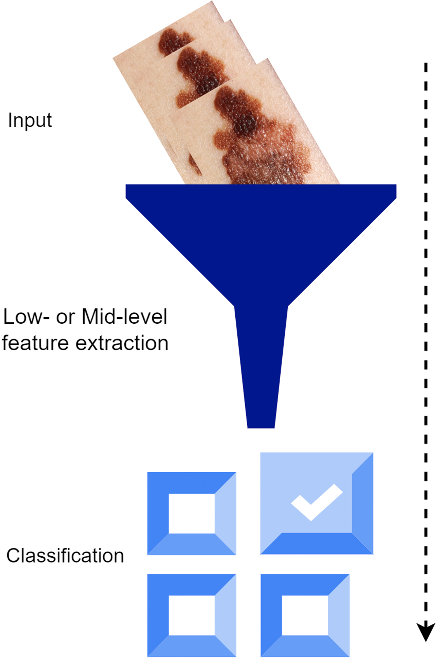
Traditional learning method.

The two distinct steps of image classification are combined into one by the DL method.^38,39 The extraction of features and classification are combined into an all-encompassing network. Compared to manually generated low- and mid-level features, the high-level features of DL depiction performed better in image recognition and classification. This idea is based on the DL model, which consists of numerous layers, ⁴⁰ including convolution, pooling, and fully linked layers. While learning more complex features, these layers transform raw data (like photos) into refined outcomes (like classification scores). DL’s main advantages lie in its ability to do two tasks (extraction of features and image classification) using a single network that has been trained from beginning to the end and in its ability to be data-driven, highly representative, task-specific, multitasked, and hierarchical.^41,42 A DL classification procedure is illustrated in Figure 2.

Figure 2.

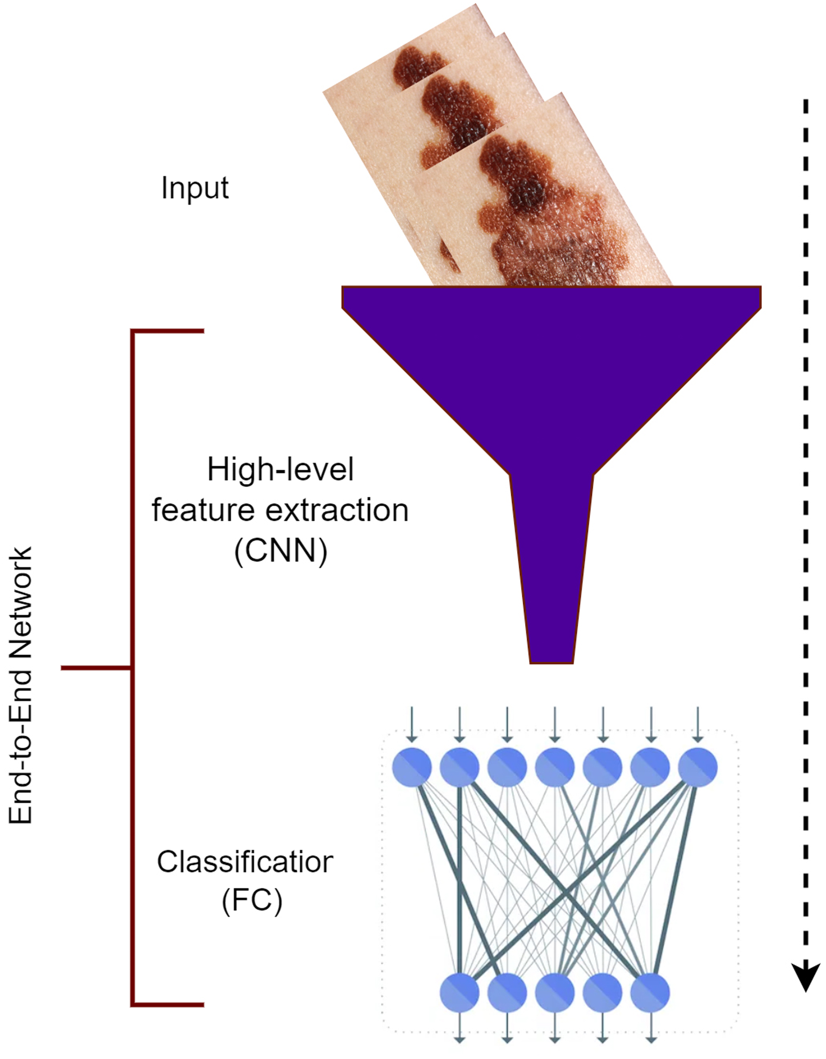
Deep learning method.

Deep learning for image classification

Image classification is one of the most fundamental problems in pattern recognition and computer vision. Some examples of applications include image and video surveillance, human-computer interface, video retrieval, and biometrics. Numerous algorithms have been developed for feature coding, which is a key constituent of image classification that has been studied for many years. The extraction of image features, followed by their classification, is what image classification is all about. ⁴³ Therefore, learning to extract and analyze image properties is crucial to image classification. The convolution, fully connected (FC), and pooling layers (PLs) that make up a CNN’s architecture are improvements above those of a regular ANN. The CNN, like the ANN, is essentially a hierarchical network. Both the function and form of layers have evolved. Convolution and PLs carry out feature extraction, whereas fully linked layers carry out classification. The classification process is, therefore, tri-layered. ⁴⁴

Convolution layer

The image may be considered a feature extraction process (out of an image) using the convolution layer. Differences between machine and human vision are discussed before moving on to the convolution layer. For instance, the dimensions, contrast, and shape of a grayscale of an apple image are all used to determine what it is. For a computer to learn a new image, it must first extract the image’s attributes from the matrix; picture convolution is one such technique. For example, a convolution kernel or a filter of size 3 $\times$ 3 can iteratively smooth out 8 $\times$ 8 images with an average step size = 1. When the filter is applied to an image, its values are multiplied by its values, and then the resulting products are combined. Consequently, the resultant value is a component of a feature matrix. After sending the whole image, the feature matrix can be retrieved. ²⁵ Figure 3 depicts the DL architecture’s Convolution Layer.

Figure 3.

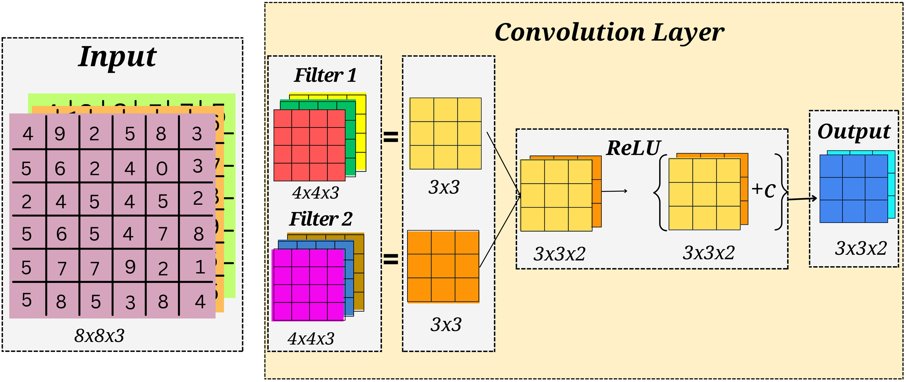
Convolution layer.

Pooling layer

Between two convolution layers, a PL is often employed in CNN. The last FC layers’ (FCL) parameter matrix and parameter set may benefit significantly from the PL’s simplification. It may be used to reduce over-fitting and expedite computation. When the learned image is too massive for the number of training parameters, a PL is added between the convolution layers. The depth of the image stays unchanged since pooling is performed in all depth dimensions. Maximum pooling occurs more often than any other kind of pooling. For instance, for a 4 $\times$ 4 matrix, the steps for max-pooling involve a filter with two broad squares and two squares high, advancing in 2-square increments across the matrix. The highest value in the filter zone is used as a component of the pooling matrix at each stage. Repeat until the filter has processed the whole matrix. ²⁴ Figure 4 represents a DL architecture PL.

Figure 4.

Pooling layer.

Fully connected layer

It is the last layer of a CNN and is often employed for classification tasks. The outputs from the previous layers are sent into this layer and then interpreted in terms of the classification job. Given that the formal pooling and convolution layers deliver five outcomes, we may split them into three distinct classes. These five outcomes are the most crucial features for determining the category to which the input image belongs. The classification job’s objectives result from three types of completely connected layers. ⁴⁵ To finish the classification task, the bias, weights, and crucial features of the FCL will carry out linear combinations resulting in three classes. Figure 5 represents an FCL.

Figure 5.

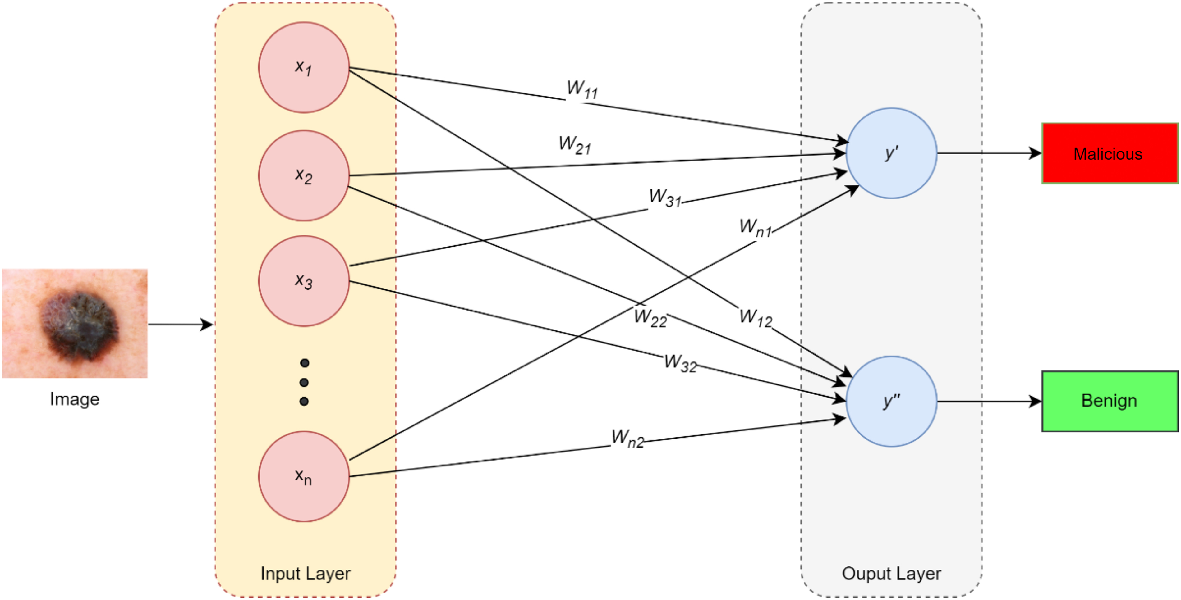
Fully connected layer.

Loss function

Before a CNN-based model can be trained to determine its loss function, the value of this function indicates how accurate a model’s prediction will be after it has been used for classification. The reliability of a model may be determined from these predicted values. The CNN-based model provides a predicted value at each processing layer during the training phase. As a result of this training, the loss function can now determine the discordance between observed and predicted data. Minimizing this loss across these two values is the primary goal of the CNN model. Cross-entropy, mean-squared error, and other loss functions are only a few examples. High values of the loss function indicate poor model performance. The loss function should have a minimum value. ⁴⁶

Deep convolutional neural network

DCNNs have emerged as a highly effective and widely used category of DL models, exhibiting exceptional performance in computer vision approaches, including the classification of images, detection of objects, and segmentation. Its inception can be attributed to Fukushima’s pioneering research on the “Neocognitron,” which drew inspiration from the hierarchical receptive field model of the visual cortex. ⁴⁷ It comprises three distinct layers: convolutional, pooling, and nonlinear. CLs may identify meaningful features by convolving a weighted kernel or filter with the input picture. These layers employ a learned set of filters to process the input image, extracting features at various scales and positions. Subsequently, the characteristics above undergo a sequence of FC strata to generate the ultimate forecast. Using nonlinear layers; the network may simulate nonlinear functions by applying an activation function on feature maps. ⁴⁸

In order to reduce the total number of model parameters, PLs are used to swap out smaller feature map neighborhoods with bigger ones. Its training entails optimizing specific parameters, commonly called weights, for defining the network’s behavior. Commonly, a variant of stochastic gradient descent is employed to update the weights by computing the discrepancy between the network’s predictions and actual labels. The selection of hyperparameters, such as the optimization algorithm and learning rate, can substantially influence the performance of a network. The units within layers exhibit local connectivity, whereby a given unit is subjected to weighted inputs from a limited neighborhood of units in the preceding layer. This neighborhood is commonly referred to as the receptive field. Higher-level layers can learn characteristics from receptive fields that are progressively broader via stacking layers, creating multi-resolution pyramids. ⁴⁹

Over the past few years, there has been a proliferation of novel deep neural architectures, such as capsule networks, transformers, spatial transformer networks, and gated recurrent units. CNNs continue to be a prevalent and extensively employed model in computer vision. It possesses a notable computational edge over FC neural networks due to weight sharing among all receptive fields in a layer, which considerably reduces parameters. ³⁶ Training DL models from the ground up for new applications or datasets may be feasible in certain situations. However, frequently there is an insufficient amount of labeled data to accomplish this. Therefore, the latest developments in deep CNNs for classification involve the application of transfer learning. This technique involves refining pre-existing models on limited datasets to enhance their efficacy. The pursuit of creating more interpretable models has gained momentum, intending to gain insights into the underlying features and patterns utilized by the network to generate predictions. ⁵⁰

Transfer learning is often employed in such scenarios to reuse a model trained for a particular task and adapt it for deployment on another similar task. In image segmentation, it is a common practice for individuals to utilize the encoder component of a neural network pre-trained on a larger dataset, such as ImageNet. Subsequently, the model is retrained using the aforementioned starting weights. According to Minaee et al., ⁵¹ pre-trained models can capture the necessary semantic information of an image for segmentation purposes. This feature enables the model to have been trained with fewer labeled instances. ResNet, AlexNet, GoogLeNet, VGGNet, DenseNet, and MobileNet are among CNN’s most widely recognized architectures. They have been used for various computer vision applications, including picture segmentation, face identification, and object detection. It has demonstrated potential in medical imaging, specifically in identifying and assessing melanoma.

In summary, deep CNNs are a potent and efficient mechanism for classifying melanoma, exhibiting cutting-edge performance across various benchmarks. The progression of the field necessitates the acquisition of more extensive and varied datasets, more easily comprehensible models, and a deeper comprehension of the fundamental biological mechanisms that underlie the development and advancement of melanoma. Through ongoing research and development, deep CNNs can potentially transform the diagnosis and treatment of melanoma and other skin cancers. The architecture of the general CNN model is presented in Figure 6.

Figure 6.

Architecture of general CNN model.

AlexNet model

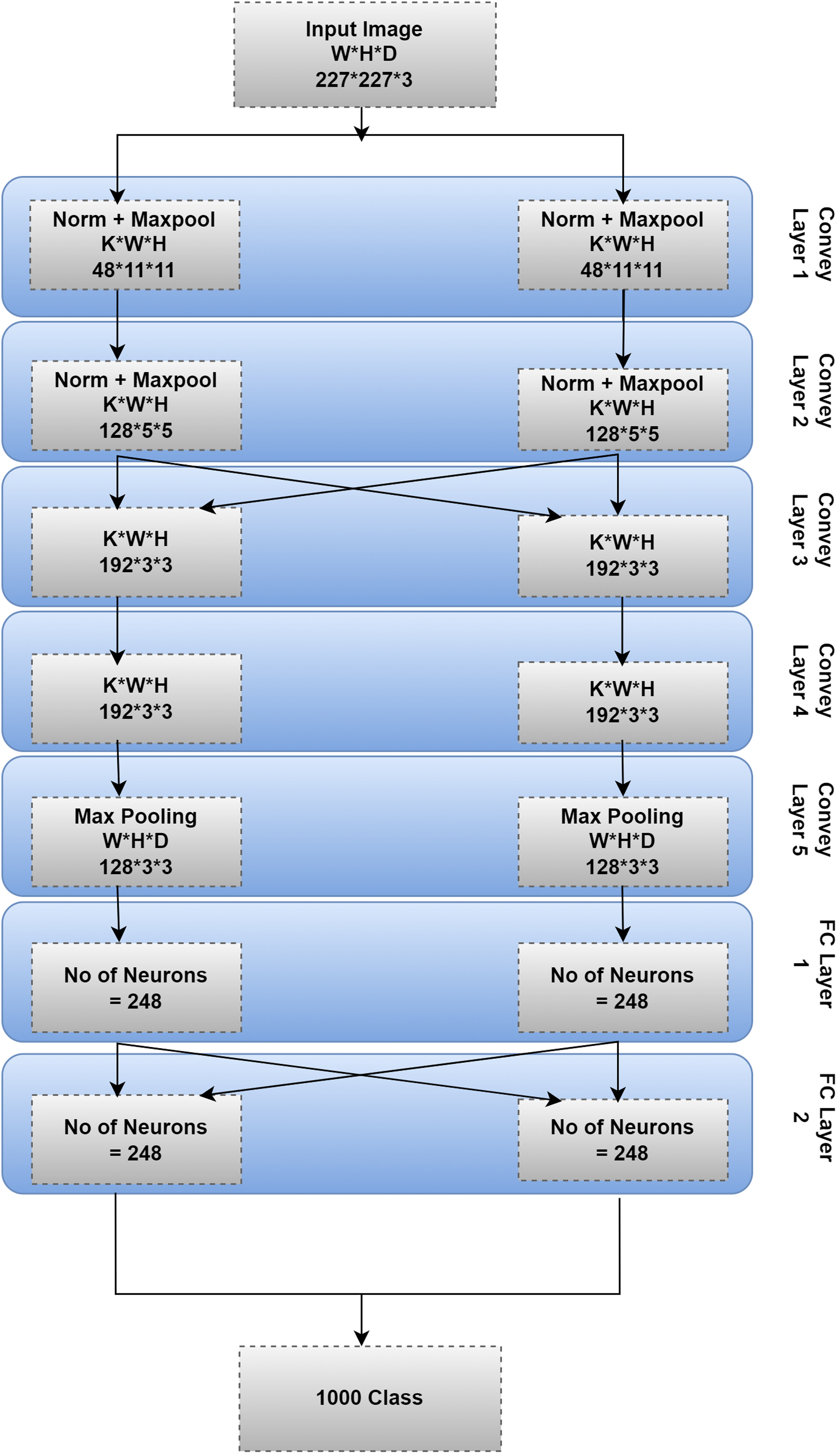
The AlexNet CNN model was created by Krizhevsky. ⁵² It was the 2012 ImageNet Large Scale Visual Recognition Challenge winner, marking a significant advancement over previous image classification methods. ⁵³ This model comprises many levels, each of which acts as an input for the ones below it. Each layer completes a particular function. The input picture was filtered using AlexNet’s first layer. Height ( $H$ ), width ( $W$ ), and depth ( $D$ ) are the three dimensions that must be present in the input picture. These dimensions’ values may be represented as 227 $\times$ 227 $\times$ 3 with $D=$ 3. The D stands for the three colors red, green, and blue. The addition of four pixels ( $s$ ) layers a color picture with multiple 96-pixel kernels ( $K$ ) and an 11 $\times$ 11-pixel filter ( $F$ ) in the first convolutional network model. In the kernel map, “stride” describes the separation between the receptive field centers of neighboring neurons. ⁵⁴ A mathematical formula (i.e., $((WF+2P)/S)$ ) is used to determine padded pixels and the convolution layer output size equal to zero, where P specifies the number of convolution layers. This layer’s output may be calculated using the formula $((227\times 11+0)/4)+1=55$ . This layer’s output serves as the following layer’s input. Since this initial layer’s job is the most important, as was already indicated, two GPUs are used to manage its workload. ⁵⁵ The PL comes next, then the CL. The PL aims to decrease each function map’s dimensionality while maintaining critical properties. Examples of pooling include sum, max, and average. ⁵⁶

Max-pooling is a layer used by AlexNet. The number of filters is 256, sent into this layer. ⁵⁷ Each filter is 55 $\times$ 256 pixels long with a 2-pixel stride. The task is split into two halves by each GPU when two GPUs are employed. The normalized and pooled output of the second CL is connected to the third CL. There are 384 kernels stacked on top of one another, each measuring 33% in size. The fourth CL produces a GPU load of 3 $\times$ 3 $\times$ 192, which uses 384 kernels of size 33 distributed across two GPUs. Each of the 256 kernels in the quarter CL has a diameter of 33 pixels and two layers will be created from them. As a consequence, each GPU will be under $3\times 3\times 280$ stress. Notably, there are no pooling or normalizing layers in the third (3rd), fourth (4th), or fifth (5th) CLs. These three (3) CLs are provided as input into a total of two fully coupled layers. Each layer has 4096 neurons in total, ²¹ as shown in Figure 7. In our case, images of skin lesions, such as melanoma, and their associated clinical data were found in the publicly accessible DermIS and DermQuest ¹ databases. The following steps are used to train an AlexNet model for melanoma image classification using these datasets:

Data preprocessing: To prepare the data for the AlexNet model, the images in the dataset may be scaled to 227 $\times$ 227 pixels. To further standardize the images, the mean pixel value of the dataset may be subtracted from each pixel.

Model training: The AlexNet model may be trained using a DL framework like TensorFlow, or PyTorch ⁵⁸ utilizing the DermIS and DermQuest datasets. Stochastic gradient descent trains the model using a 0.001 learning rate and a 32-iteration training batch. The model may be trained for a considerable amount of time (epochs) before reaching a steady state of accuracy.

Model evaluation: Testing the trained model with data not utilized during training yields an evaluation of the model’s performance. One may measure the model’s efficacy by calculating its accuracy, precision, recall, and F1 score.

Figure 7.

Architecture of Alexnet.

A brief description of the AlexNet model layers is given in the following sections.

Convolution network layer

The input data is processed by a collection of learnable filters (AKA kernels or weights) in a neural network’s CL (AKA a convolution layer or simply conv layer). The filters are convolved over the input image to create the output feature maps. It is the most crucial layer in DL neural network models for creating and refining feature maps. We integrated the input at each point after performing matrix multiplication. ¹⁹

In order to obtain a single output value for each location in the feature map, the convolution procedure entails sliding each filter window across the input picture, multiplying the filter values by the pixel values in the corresponding window, and summing the results. It is done for each filter, resulting in an array of feature maps. The neural network’s output feature maps are fed into the next layer. ³⁶

CLs excel in image processing because they can be trained to identify features, such as corners, edges, and textures within the input data. The network can learn more sophisticated representations of the input data by layering CLs on top of one another. ⁵⁹

CLs may be used to extract characteristics from the input images (i.e., suggestive of melanoma) in melanoma image classification using the DermIS and DermQuest datasets. The network is trained to identify melanoma-specific patterns and structures, such as non-uniform shapes and colors and uneven or blurry boundaries, by applying a set of learnable filters to the input images and convolving over the image. Using these characteristics, the images may be labeled as melanoma or benign.

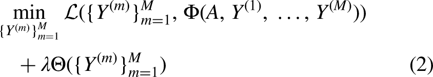
Mathematical modeling

A linear transformation is applied by each layer in a hierarchical DL model with subsequent non-linear preceding layers. ⁶⁰ Let the input be represented as $A\in {\mathbb{Z}}^{P\times Q}$ . The rows in matrix $A$ represent data points with $Q$ -dimensions, such as $Q$ -pixel grayscale images and the number of training instances is denoted as $P$ . Assuming that the output of layer $m-1$ , denoted as $A^{(m-1)}\in {\mathbb{Z}}^{P\times q_{m-1}}$ , undergoes a linear transformation to produce $A^{(m-1)}{Y}^{(m)}\in {\mathbb{Z}}^{P\times q_m}$ (a $q_m$ -dimensional representation) at layer $m$ , where $Y^{(m)}\in {\mathbb{Z}}^{q_{m-1}\times q_m}$ reflects this transformation. Each column of $Y^{(m)}$ represents an operation like a linear classifier in FC networks or convolution with a filter in a CNN. Assuming a non-linear activation function ${\mathrm{\Psi }}^{(m)}:\mathbb{Z}\to \mathbb{Z}$ , such as the sigmoid ${\mathrm{\Psi }}^{(m)}(a)=(1+e^{-a}{)}^{-1}$ , the hyperbolic tangent ${\mathrm{\Psi }}^{(m)}(a)=\tanh (a)$ , or the Rectified Linear Unit (ReLU) ${\mathrm{\Psi }}^{(m)}(a)=max\{0,a\}$ , for each entry in $A^{(m-1)}{Y}^{(m)}$ , the $m$ th layer of the neural network is generated as $A^{(m)}={\mathrm{\Psi }}^{(m)}(A^{(m-1)}{Y}^{(m)})$ . Thus, the output of the network, $A^{(M)}$ , can be expressed as equation (1).

$$\begin{array}{rl}& \mathrm{\Phi }(A,Y^{(1)},\dots ,Y^{(M)})\\ & ={\mathrm{\Psi }}^{(M)}({\mathrm{\Psi }}^{(M-1)}(\dots {\mathrm{\Psi }}^{(2)}({\mathrm{\Psi }}^{(1)}(A{Y}^{(1)})Y^{(2)})\dots Y^{(M-1)})Y^{(M)})\end{array}$$

(1)

To clarify, $\mathrm{\Phi }$ is a matrix of dimensions $P\times C_L$ , where $C_L=q_M$ represents the number of classes in a classification task and is the dimension of the network’s output. The mapping $\mathrm{\Phi }$ can be interpreted as a function of network weights denoted by $Y=Y^{(m)}{\}}_{m=1}^M$ , with the input value $A$ held constant. Alternatively, $\mathrm{\Phi }$ can be seen as a function of input data with constant weights $Y$ . The problem of learning the parameters in a deep neural network involves $P$ training instances of the form $(A,Y)$ , where the learning problem is expressed as $Y=\{Y^{(m)}{\}}_{m=1}^M$ . In a classification setting, the data points ( $A$ in ${\mathbb{Z}}^{P\times Q}$ ) are represented by rows, and the class membership is indicated by the rows of $Y\in \{0,1{\}}^{P\times C_L}$ , where $Y_{j,c_l}=1$ if the $j$ th row of $A$ belongs to class $c_l\in \{1,\dots ,C_L\}$ , and $Y_{j,c_l}=0$ otherwise. The rows of $A$ serve as independent variables in a regression context, while the rows of $Y\in {\mathbb{Z}}^{P\times C_L}$ are dependent variables. To solve the network learning problem, the weights $Y$ can be derived as an optimization problem using equation (2).

$$\underset{\{Y^{(m)}{\}}_{m=1}^M}{min}\mathcal{L}(\{Y^{(m)}{\}}_{m=1}^M,\mathrm{\Phi }(A,Y^{(1)},\dots ,Y^{(M)}))+\lambda \mathrm{\Theta }(\{Y^{(m)}{\}}_{m=1}^M)$$

(2)

where the loss function $\mathcal{L}$ measures the agreement between the actual ( $Y$ ) and predicted outputs ( $\mathrm{\Phi }$ ), and the regularization term $\mathrm{\Theta }$ is designed to prevent overfitting, for example, through $L_2$ regularization ( $\mathrm{\Theta }(\{Y^{(m)}{\}}_{m=1}^M)=\sum _{m=1}^M\Vert Y^{(m)}{\Vert }_F^2$ ) and a balancing parameter $\lambda >0$ .

Rectified linear unit layer

CNNs often use the ReLU activation function for image identification applications. ⁶¹ All the negative pixel values in a picture are transformed to zero by this non-linear function, while the positive values remain unaltered. It improves the network’s ability to learn and the speed of image classification. Non-linearities are handled well by this layer. It is now applicable to the feature map generated by the CL. In melanoma detection, this layer aids in identifying irregular borders, a significant malignancy indicator. It enables features corresponding to serrated or asymmetric edges of skin lesions when analyzing dermoscopic images. This capability aids dermatologists in accurately locating potentially malignant melanomas, resulting in timely treatment. The ReLU activation function may be expressed mathematically as shown in equation (3) below:

$$f(i)=max(0,i)$$

(3)

Where $i$ is the layer’s input and $f(i)$ is the layer’s output after the ReLU activation function has been applied. Whenever the input is a positive number, the function returns that number; otherwise, it returns 0.

In a typical CNN architecture, the ReLU layer is employed right after the CL. The ReLU layer takes the output of the CL and applies the activation function to each element of that output. It helps the network learn more robust and discriminatory features by producing a feature map with only positive values. In conclusion, the ReLU layer is a non-linear activation function that aids in introducing non-linearity in the CL’s output of a CNN. Due to its ease of use, efficiency, and ability to significantly boost neural network performance has quickly become the DL method of choice. ⁶²

AlexNet, like many other CNNs, uses the ReLU layer as an activation function. After each CL and FCL in AlexNet, ReLU is employed as the activation function. To help the network learn more nuanced characteristics and patterns, the ReLU layer introduces some non-linearity. The ReLU activation function is employed at the end of each CL and the FCL in AlexNet for melanoma image classification using the DermIS and DermQuest datasets. It aids in the detection of picture characteristics that may point to the existence of melanoma. Adding a ReLU layer, which introduces non-linearity to the network, may help the model acquire more sophisticated and abstract representations of the pictures, leading to better melanoma classification performance. ⁶³

The ReLU activation function is employed at the end of each CL and the FCL in AlexNet for melanoma image classification using the DermIS and DermQuest datasets. It aids in the detection of picture characteristics that may point to the existence of melanoma. Adding a ReLU layer, which introduces non-linearity to the network, may help the model acquire more sophisticated and abstract representations of the pictures, leading to better melanoma classification performance. ⁶⁴

Maximum pooling layer (MPL)

The suggested architecture incorporates a PL after the initial and subsequent convolution layers, as well as after the fifth convolution layer, to lower the spatial size of each frame and, by extension, the computing cost of the proposed model. For example, diagnosing melanoma facilitates extracting high-level characteristics, such as pigment variances and overall lesion structure. It facilitates efficient analysis of dermoscopic images by discarding irrelevant details while retaining essential characteristics. In most cases, the pooling procedure will average the values across all picture slices or choose the highest. In the proposed study, we use pooling by comparing the most significant value against each slice. A MPL is a down-sampling process that preserves the most salient features while decreasing the feature map’s overall spatial size. This procedure aims to find the most significant value in each non-overlapping rectangle of the input feature map. In the end, a new feature map is found that is smaller, having the same number of channels as the original feature map. ⁶⁵

The MPL’s primary role is to make the feature map translation invariant. It implies that the network can identify the same feature in multiple picture regions, despite the feature being rotated or translated. The network takes the most significant value within a narrow rectangular section of the feature map, which guarantees recognition even if the feature is slightly shifted in the picture. After the CLs of the AlexNet model, a MPL was employed to compress the feature maps while keeping the most relevant features. ⁶⁶ After the first, second, and fifth CLs in AlexNet, a MPL was employed with a 3x3 filter and a stride of 2. After the CLs, the MPL may be utilized to minimize the spatial size of the feature maps while maintaining the most relevant characteristics for melanoma image classification using the DermIS and DermQuest datasets.

The MPL’s size may be modified based on the input picture size and the desired feature map output size. Decreasing the impact of overfitting and enhancing the network’s translational invariance may enhance the model’s accuracy. For melanoma image classification, the MPL may be employed to maintain essential information while decreasing the dimensionality of feature maps produced by CLs. Overfitting is avoided, and model performance is enhanced. For example, a MPL may be used in a CNN trained to classify melanoma images after the output of a CL has identified relevant characteristics (such as edges, forms, or patterns). This layer will take the maximum value from each feature map’s non-overlapping rectangles and output the set. ⁶⁷

The MPL may shrink the feature maps produced by the CLs used in melanoma image classification without losing valuable information. Better success in categorizing melanoma images may result from the model being better able to generalize and prevent overfitting.

Response normalization layer and soft-max activation

Another layer in CNN is the response normalization (RN) layer, sometimes called local response normalization. It is used on the ReLU layer’s output to standardize the findings and boost the model’s generalization capacity. Testing errors for the proposed network are reduced by response normalization after the initial two sessions. The input layers of the network and the network as a whole are both normalized by this layer. By highlighting the variations across activation maps, RN helps to mitigate overfitting. ⁶⁸ Variable brightness and contrast conditions impact image quality in real-world scenarios. This layer assures consistent melanomas identification across a variety of environments. This layer standardizes output activations, enabling accurate diagnosis regardless of lighting variations, for instance, when analyzing skin lesion images captured under varying lighting conditions.

Soft-max activation

Soft-max works on top of the activated functions. The probabilities for a given classification are improved by feeding the results of the convolutional network layer’s performance after five series into the Soft-max layer enabling multi-class classification. For example, it plays a crucial role in allocating probabilities to each class, allowing the model to identify and classify various skin conditions accurately. This capability enables dermatologists to make informed decisions regarding treatment plans based on accurate lesion-type identification. The neural network output may be transformed into a probability distribution across the expected output classes using the Soft-max activation function. ⁶⁹ The last classification layer sorts the images into different frames using these probabilities. A vector of real-valued scores (such as the output of the last FCL in a neural network) is accepted as input by the Soft-max function. It returns a vector of the same size, where each element reflects the likelihood of classifying the input. To generate an N-dimensional vector of real values between 0 and 1 that sum to 1, the Softmax function $SA(n)$ uses the formula provided in equation (4).

$$S{A}_j(i)=\frac{e^{i}j}{\sum {n=1}^N{e}_n^i}$$

(4)

Where $j$ is the output vector element index, and $n$ is the input vector element index, used to generate an $N$ -dimensional vector with real values ranging from 0 to 1. The exponential values of each input vector element are added together to generate the denominator of the formula. The Soft-max function is used for the problem of melanoma classification to determine the likelihood that an input picture belongs to each of many classifications, such as benign and malignant. The prediction is then assigned to the category with the greatest probability. ⁷⁰

Dropout layer

Overfitting in CNN models may be avoided using the dropout layer. As the number of iterations grows in this study, overfitting and depiction of neurons are readily managed thanks to the dropout layer. Model averaging using neural networks is a powerful method for normalizing training data. ⁷¹ Using CL kernel sizes, MPLs, and skipping factors, the function maps at the output are downsampled to one pixel per map. The tightly linked layer also limits the uppermost layers’ performance to a one-dimensional function vector. High-level characteristics retrieved from the training data may be used by the higher layer, which is typically completely coupled to the output device for class labeling. Dropout is a DL approach intended to avoid overfitting, which happens when a model becomes too specific to its training data and cannot accurately predict new data. ⁷² To train a smaller, simpler network, the dropout layer eliminates (sets to zero) a random number of neurons in a layer. It makes the network more stable and less susceptible to overfitting by lowering its dependency on any one neuron. The tightly linked layer, where each neuron connects to every other neuron, is often put before the dropout layer. Each FCL neuron has a dropout probability of p during training. The standard range for this probability is between 0.2 and 0.5. ⁷⁰

The dropout layer prevents overfitting when classifying melanoma, for instance, by encouraging the network to learn a broader range of features, thereby improving its ability to diagnose various real-world skin lesions. This phenomenon, during training, can be elaborated as choosing a percentage $pr$ of images at random to be discarded from each training sample. To keep the anticipated value of each neuron constant, multiply the remaining neurons by $1/(1-pr)$ . To the following layer, please provide the resultant vector. While during trials, improvements in neural network performance on tasks, such as image classification and natural language processing, have been attributed to using the dropout layer. It improves a neural network’s ability to learn from new data and perform better on unknown instances by lowering the likelihood of overfitting. ⁷³

Similarly, during the training process, let $O_t$ represent the output of the layer that came before it, and let $B_i$ represent a binary vector of the same dimension as $h$ , with each element having a probability of 0 with the dropout rate of $dr$ and a probability of 1 with the dropout rate of $(1-dr)$ , where $dr$ is the dropout rate. The Dropout layer’s masked output $O_t^{\prime }$ is thus defined as shown in equation (5).

$$O_t^{\prime }=O_t*B_i/(1-dr)$$

(5)

During the inference process, the Dropout layer is turned off, and the output $O_t$ is scaled by $(1-dr)$ to account for the missing dropout units and can be computed using equation (6).

$$O_t^{\prime }=O_t*(1-dr)$$

(6)

Overfitting in DL models may be avoided with the regularization method dropout. During training, some neurons are randomly removed (or set to zero) to ensure the network learns redundant material representations. Decreasing neuronal interdependence and blocking complicated co-adaptations on training data enhances the network’s generalization capability. Dropout layers may be utilized to enhance the effectiveness of DL models for melanoma classification. Introducing dropout layers may enhance the overall performance and generalization capacity of DL models for melanoma classification. ⁷⁴

Proposed architecture and model

This section details the proposed fine-tuned CNN-based model for melanoma identification and classification.

The proposed classification model

The proposed model’s objective is to identify and classify melanoma images. Figure 8 illustrates the block diagram of the proposed model. Initially, features are extracted by pre-trained neural convolution networks (i.e., Alex Net with Soft-max layer and the same with SVM classifier). In the second step, transfer learning is applied using the pre-trained Alex Net CNN for the classification. To get the best classification performance, the outcomes of both methodologies are compared. The proposed model has many phases, and the subsequent sections describe the steps used in each phase.

Figure 8.

Proposed architecture.

The pre-processing phase

This phase is responsible for two tasks. First, each image is scaled to fit the CNN model specifications. Further, the pictures in grayscale are converted into color ones. For all of the images in each dataset, data augmentation is used. Data augmentation involves three tasks: Image enhancement, orientation (i.e., randomly, horizontally, and vertically), and flipping.

The feature extraction phase

Two pre-trained convolution neural networks, MII-SFMAX models and MI-SVM, are applied in this phase. For extracting the features, Alex Net with SVM makes up the MI-SVM model, while Alex Net with the Softamx layer makes up the MII-SFMAX model is used.

The fine-tuning of hyperparameters

The accuracy and precision of DL models used for diagnosis may be significantly increased when they are fine-tuned in the context of melanoma categorization. Fine-tuning is a DL technique used to improve the performance of DL-based models by making little adjustments. The AlexNet model’s accuracy has increased when used for melanoma classification. The AlexNet model has five CLs, ReLU activation functions, and response normalization layers to best extract input image features and trains the dataset. The input dataset is divided into an 80:20 ratio, and then the images are scaled and converted from grayscale to color channels, as mentioned before. The network receives the pre-processed images and uses the top five layers of the pre-trained model to extract the most features possible. In order to fine-tune the network for optimal accuracy, the last three levels are changed. In-depth testing determines the training hyper-parameters, including different batch sizes and stochastic gradient descent with momentum (SGDM). Figure 9 illustrates the fine-tuning procedure. The utilization of SGDM is employed for minimizing the loss function. The SGDM algorithm updates a network model’s bias and weights hyper-parameters by iteratively adjusting them in a negative loss gradient direction. This adjustment is carried out through incremental movements. Mini-batch is a commonly employed technique in SGDM ⁷⁵ to facilitate incremental steps toward minimizing the loss function. The Mini-Batch Size refers to the magnitude of the mini-batch employed during each training iteration. Its purpose is to assess the modification of the hyper-parameters utilized and the loss function gradient the supplementary momentum results in a decrease in oscillations. The SGDM employs a uniform learning rate for all hyper-parameters. The learning rate can be either constant or variable. Selecting a small value for the parameter may result in a prolonged training process, while opting for an immense value may lead to suboptimal outcomes or divergence. The utilization of the maximum number of epochs is implemented to ensure the brevity of the training process. A comprehensive testing process was conducted to ascertain the optimal epoch size. The term “epoch” pertains to the final iteration of the training procedure conducted on the complete training dataset. The FCLs’ dimensions were adjusted to correspond with the number of categories in the dataset. The WeightLearnRateFactor and BiasLearnRateFactor values were increased for FCLs to expedite the learning process in newly added layers relative to those transferred. The tuning of the hyper-parameters as presented in Table 2:

Figure 9.

Fine-Tuning.

Table 2.

Details about AlexNet hyper-parameters.

Parameter	Value
Epochs	60
Validation step	6
Optimizer	Stochastic gradient descent momentum (SGDM)
Learning rate	$1\times {10}^{-4}$
Decay	Default
Momentum	Default

Parameters fine-tuned

During the model development process, several parameters were fine-tuned to optimize the performance of the proposed melanoma detection architecture. The following parameters were systematically explored to achieve the best possible results:

Number of layers and filters: The depth of the network was adjusted by iteratively adding or removing layers. Additionally, various configurations for the number of filters in each CL were evaluated. These adjustments aimed to balance model complexity and effective feature extraction.

Activation functions: Different activation functions, including ReLU, Leaky ReLU, and exponential linear units, were investigated for each layer. The selection of appropriate activation functions was crucial in addressing vanishing gradient problems and enhancing model convergence.

Batch size: The impact of batch size on training dynamics and generalization was explored. Different batch sizes were tested, focusing on balancing computational efficiency and convergence speed. Smaller batch sizes were also evaluated for potential improvements in model generalization.

Learning rate: The learning rate, a fundamental hyperparameter in gradient-based optimization, was fine-tuned to achieve optimal convergence. Fixed and adaptive learning rate scheduling techniques were investigated within the typical range of 0.001 to 0.1.

Dropout rate: Dropout layers, employed to mitigate overfitting, were optimized by fine-tuning the dropout rate. Values ranging from 0.2 to 0.5 were tested, and the impact of dropout regularization on model performance was carefully observed.

Loss function: Choosing an appropriate loss function is vital for the specific classification task. The suitability of various loss functions, including binary cross-entropy, was considered, and potential adaptations of loss functions were explored to address challenges unique to melanoma detection.

Validation split: Various validation split ratios were examined to allocate an appropriate proportion of data for training and validation. Common splits, such as 80-20 or 70-30 for training and validation, were assessed for their influence on model generalization.

Data augmentation techniques: Various data augmentation techniques, including rotations, flips, and brightness adjustments, were applied to the training dataset. These techniques aimed to enhance the model’s robustness and alleviate issues related to limited training data.

Transfer learning strategy: Transfer learning from pre-trained models was explored to leverage features learned from similar tasks. The selection of a suitable pre-trained model, layers frozen during transfer, and additional fine-tuning of the architecture was considered.

Regularization techniques: Regularization techniques such as L2 regularization and weight decay were investigated to control model complexity and prevent overfitting. Their influence on the balance between bias and variance was carefully assessed.

Hyperparameter grid search: A systematic grid search approach was employed to fine-tune hyperparameters. The ranges of values tested for each parameter were determined empirically, and trends observed during the grid search were used to make informed decisions.

Early stopping: Early stopping, a technique to prevent overfitting, was employed with a carefully chosen criterion. This technique helped ensure the model converged without excessively fitting the training data.

Results of hyperparameter tuning: Throughout the fine-tuning process, the impact of each parameter on validation performance was rigorously evaluated. Insights were gained into the trade-offs between model complexity, training time, and generalization.

The fine-tuning process was pivotal in achieving the optimal architecture for melanoma classification, enabling the model to effectively learn relevant features from the input images and generalize to new, unseen data.

Image classification

Image classification has been carried out using the SVM and CNN classifiers. Two pre-existing and fully developed neural convolution networks, Alex-net with Soft-max layer and Alex Net with SVM classifier were used to extract features. A single classifier is utilized in both networks. The SVM is a classification algorithm that can be utilized for transfer learning purposes in conjunction with the pre-existing Alex Net CNN and the associated Soft-max layer classification task. The two CNN models were tested using three distinct datasets, and the outcomes were observed to be of considerable significance. Given their demonstrated efficacy in addressing pattern recognition and machine learning challenges, this study employs SVM and Soft-max classifiers as image classifiers.

Algorithm 1

Melanoma image classification.

Require: d {Input melanoma image dataset of size $M\times N$ }

1: Begin

2: $d.load()$

3: $d.preprocess()$

4: while do

5:    $fp\leftarrow d.convolute[F,K,K]$

6:   tensor= ${\text{generate}}_{tensor}(M-K+1)\times (\text{N}-\text{K}+1)\times \text{P}$

7:    $fp.activation(relu)$

8:    $d.split(train,test)$

9:    $d.maxpooling(fp)$

10:   tensor= ${\text{generate}}_{tensor}(M-K+1)/S\times (\text{N}-\text{K}+1)/\text{S}\times \text{P}$

11: end while

12: $f{p}_{singl{e}_{dim}}\leftarrow Flatten(d,fp)$

13: $I\leftarrow layer.add(f{p}_{singl{e}_{dim}},activation=relu)$

14: $pd\leftarrow layer.add(I,activation=softmax)$ Image classification predictions

Algorithm 1 explains the mechanism of image classification for melanoma detection. Each step is elaborated below: The convolution operation is applied to the input image.

Apply convolution operation to the input image: In this step, the datasets of melanoma images (i.e., DermIS and DermQuest) are given as input. The input image, size $M\times N$ , is convolved with a set of learnable filters to produce feature maps. Each filter is a $C\times K\times K$ -dimensional tensor, where $K$ is the size of the filter, and $C$ is the number of color channels. Convolution computes the dot product of the filter with every $C\times K\times K$ subregion of the input image. It produces a feature map: a $(M-F+1)\times (N-F+1)\times P$ tensor, where $P$ is the number of filters. This operation is repeated for each filter in the set to produce a stack of feature maps stored in a $feature\mathrm{\_}maps$ list. To introduce nonlinearity into the model, the proposed model uses a nonlinear activation function (such as ReLU) for each element of the feature maps following the convolution operation. This step produces a list of feature maps with dimensions $(M-K+1)\times (N-K+1)$ .

Apply maximum pooling to each feature map: In this step, we reduce the spatial size of each feature map by applying a max pooling operation. Max pooling divides the feature map into subregions of size $F\times F$ that do not overlap and determines the maximum value within each subregion. It generates a pooled feature map, a two-dimensional tensor with dimensions $(M-K+1)/Sx(N-K+1)/S$ , where $S$ is the pooling operation’s stride. This operation is repeated for each feature map in the $feature\mathrm{\_}maps$ list to produce a new list of pooled feature maps stored in the $pooled\mathrm{\_}feature\mathrm{\_}maps$ list. After the max pooling operation, the first and second steps are repeated for multiple layers to form a deep CNN architecture. The same operations are performed in each successive layer using a new set of learnable filters on the pooled feature maps generated by the previous layer.

Flatten the output of the final layer of pooling: In this step, the output of the final PL is transformed into a 1-dimensional feature vector. It involves transforming the $(M-K+1)/S\times (N-K+1)/S\times P$ tensor into a vector with the same dimensions.

Feed the fully-connected feature vector to a layer with learnable weights and biases: This step feeds an FCL with learnable weights and biases the feature vector. This layer computes the dot product of the feature vector and an $(M-K+1)/S\times (N-K+1)/S\times P\times D$ weight matrix, where $D$ is the number of neurons in the FCL. On the output of the dot product, we add a bias term of length $D$ and apply a nonlinear activation function (such as ReLU). It yields a vector of length $D$ that we refer to as $fully\mathrm{\_}connected$ .

Apply a nonlinear activation function to the FCL’s output: In this step, non-linearity is introduced into the model by applying a nonlinear activation function (such as ReLU) to the output of the FCL. It results in a vector of probabilities for every class, which we refer to as $predictions$ . The final output of the algorithm is the $predictions$ vector, which represents each class’s predicted probability.

Formal description of CNN-based image classification model

This section gives a formal, detailed description of the CNN-based melanoma image classification model, including the specific operations and calculations done at every phase of the model.

Assumptions : Let the size of the input image $X$ is $M\times N\times C$ , where $M$ is the height, $N$ is the width, and $C$ is the number of color channels. The model’s result is a vector called $Y\mathrm{\_}hat$ with length $K$ , where $K$ is the number of classes to be sorted. In our case, $K$ = 10. The model is made up of $L$ layers. Each layer starts with a set of filters, then a max pooling operation, and finally, a ReLU activation function. The last layer is a FCL with a ReLU activation function, followed by a softmax activation function. Operation of Convolution: Let $W\mathrm{\_}1$ be a set of learnable filters with the size $F\times F\times C\times P$ , where $F$ is the size of the filter, $C$ is the number of input channels, and $P$ is the number of output channels. Let $b\mathrm{\_}1$ be a biased term with $P$ length. Let $Z\mathrm{\_}1$ be the result of applying convolution to $X$ with $W\mathrm{\_}1$ and $b\mathrm{\_}1$ : $Z\mathrm{\_}1=ReLU(convolve$ $(X,W\mathrm{\_}1)+b\mathrm{\_}1)$ , where the convolution operation is convolved. Max Pooling Procedure: Let $S$ be the max pooling operation’s step size. Let $Z\mathrm{\_}2$ be the result of applying the max pooling operation to each feature map in $Z\mathrm{\_}1$ : $Z\mathrm{\_}2=max\mathrm{\_}pool(Z\mathrm{\_}1,F,S)$ , where $max\mathrm{\_}pool()$ is the max pooling operation. Several levels: To make a deep CNN architecture, repeat the convolution and max pooling steps for $L-1$ further layers. Flatten: Let $Z\mathrm{\_}L$ result from the last layer of max pooling. Let $Y$ be a vector of length $(M-F+1)/S\times (N-F+1)/S\times P$ that is made by flattening $Z\mathrm{\_}L$ : $Y=flatten(Z\mathrm{\_}L)$ . FCLs: Let $W\mathrm{\_}2$ be a weight matrix with the size $((M-F+1)/S)\times ((N-F+1)/S)\times$ $P\times D$ , where $D$ is the number of neurons in the FCL. Let $b\mathrm{\_}2$ be a biased term that is $D$ long. $Z\mathrm{\_}3$ is the output of the FCL: $Z\mathrm{\_}3=ReLU(Y\times W\mathrm{\_}2+b\mathrm{\_}2)$ . Layer Three: Let $W\mathrm{\_}3$ be a $D\times K$ weight matrix, where $K$ is the number of classes that need to be sorted. Let $b\mathrm{\_}3$ be a biased term that is $K$ long. Let $Y\mathrm{\_}hat$ be the output of the output layer: $Y\mathrm{\_}hat=softmax(Z\mathrm{\_}3\times W\mathrm{\_}3+b\mathrm{\_}3)$ , where $softmax()$ is the softmax activation function. This model uses CLs and FCLs to learn features from an image and put it into one of $K$ possible classes. The FCLs do the final classification, while the CLs pull out features from the image. The ReLU activation function makes the model nonlinear, and the softmax activation function is used to turn the model’s output into a probability distribution over the $K$ classes.

Example : Let us say we have an image of size 224 $\times$ 224 $\times$ 3 ( $M=224$ , $N=224$ , and $C=3$ ) that we want to classify as either benign or malignant ( $K=2$ ). Operation of Convolution: Let $W\mathrm{\_}1$ be a 3 $\times$ 3 $\times$ 3 $\times$ 64-size set of filters that can be learned with $F=3$ , $C=3$ , and $P=64$ . Let $b\mathrm{\_}1$ be a 64-letter bias term. Let $Z\mathrm{\_}1$ be the result of applying convolution to $X$ with $W\mathrm{\_}1$ and $b\mathrm{\_}1$ : $Z\mathrm{\_}1=ReLU(convolve(X,W\mathrm{\_}1)+b\mathrm{\_}1)$ , where the convolution operation is convolved. Max Pooling Procedure: Let $S$ be the max pooling operation’s step size, and we can choose $S=2$ . Let $Z\mathrm{\_}2$ be the result of applying the max pooling operation to each feature map in $Z\mathrm{\_}1$ : $Z\mathrm{\_}2=max\mathrm{\_}pool(Z\mathrm{\_}1,F=2,S=2)$ , where $max\mathrm{\_}pool$ is the max pooling operation. Several levels: We can keep convolution and max pooling for several more layers to make a CNN architecture with many layers. For example, we could add another CL with 128 filters, then a MPL with stride 2. Flatten: Let $Z\mathrm{\_}L$ be the output of the last MPL. Its size will be 7 $\times$ 7 $\times$ 128 if we add the extra layer we talked about above. Let $Y$ be a 7 $\times$ 7 $\times$ 128-element vector with the length 6272 that is made by flattening $Z\mathrm{\_}L$ : $Y=flatten(Z\mathrm{\_}L)$ . Layer That is FC: Let $W\mathrm{\_}2$ be a 6272 $\times$ 256 weight matrix, where $D=256$ . Let $b\mathrm{\_}2$ be a 256-bit biased term. $Z\mathrm{\_}3$ is the output of the FC layer: $Z\mathrm{\_}3=ReLU(Y\times W\mathrm{\_}2+b\mathrm{\_}2)$ . Layer Three: Let $W\mathrm{\_}3$ be a 256 $\times$ 2 weight matrix with $K=2$ . Let $b\mathrm{\_}3$ be a 2-length biased term. Let $Y\mathrm{\_}hat$ be the output of the output layer: $Y\mathrm{\_}hat=softmax(Z\mathrm{\_}3\times W\mathrm{\_}3+b\mathrm{\_}3)$ , where $softmax()$ is the softmax activation function.

Note that the actual values for the weights and biases would be learned during the training process in this example. However, these are the shapes and sizes of the variables used in the model.

Experimentation and results

This section details the experimentation setup and results.

Experimental setup

The proposed melanoma classification model is implemented for evaluation purposes. The model is implemented on a system with CPU i7 eighth generation clock speed 2.5GHz. Python 3.0 is installed on the system. The dataset was loaded to Google drive. The Google drive was mounted with CoLab. The Colab is an online platform for implementing Python projects (Table 3).

Table 3.

Table of experimentation parameters.

Simulation parameters	Value
System	i7-8th generation
Storage	500GB
Programming	Python
Online platform	Google Colab
GPU	NVIDIA Tesla K80
Framework	Keras

Dataset description

This study used DermIS, DermQuest, their combination DermIS&Quest, and ISIC2019 datasets. The number of images in these datasets differs in their original form and after augmentation. For example, the DermIS dataset had 69 samples when first made; however, after it was augmented, it had 621 samples. In the same way, there were originally 137 sample images in DermQuest; however, after augmentation, there were 1233. In DermIS&Quest, there were 206 original samples and 1854 images that had been augmented. In ISIC2019 dataset has 25,331 instances based on HAM10000 and $BCN\mathrm{\_}20000$ datasets. It possesses high-quality images of 10015 RGB images having 600 $\times$ 450-pixel resolution, while the $BCN\mathrm{\_}20000$ has RGB images having 1024 $\times$ 1024-pixel resolution. ⁷⁶ We split each dataset into a training set and a testing set so that we could train and test our classification model. A ratio of 80:20% is used for both training and testing, respectively. It ensures the model is trained on a large enough dataset and can work well with samples it has not seen before. Table 4 gives information about the datasets.

Table 4.

Dataset name and number of images.

Datasets	No. of images
DermIS	621
DermQuest	1233
ISIC2019	25000

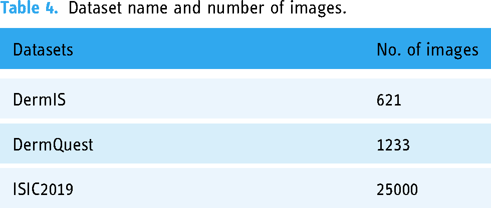
Figure 10 represents some of the images from the DermIS dataset. This dataset consists of images related to melanoma and nevus diseases. These images are not augmented or rotated but are in their original characteristics.

Figure 10.

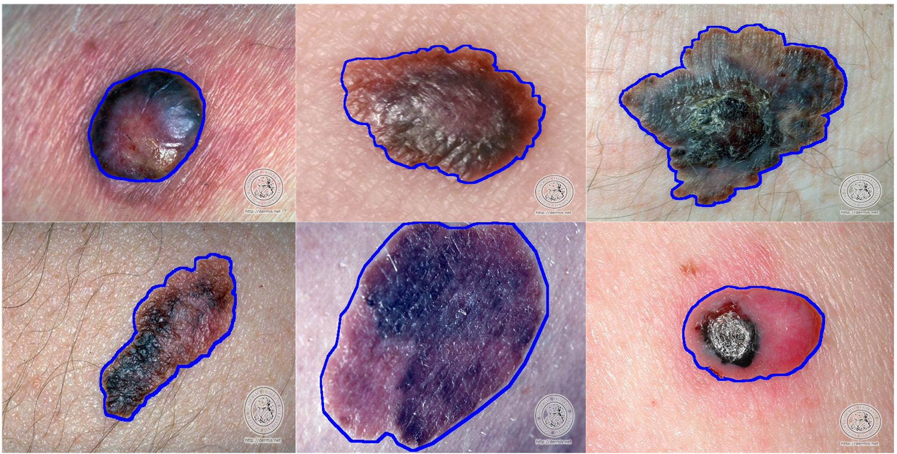
Image samples from DermIS dataset.

Figure 11 represents some of the images from the DermQuest dataset. This dataset consists of images related to melanoma and nevus diseases. These images are not augmented; these are in their original characteristics.

Figure 11.

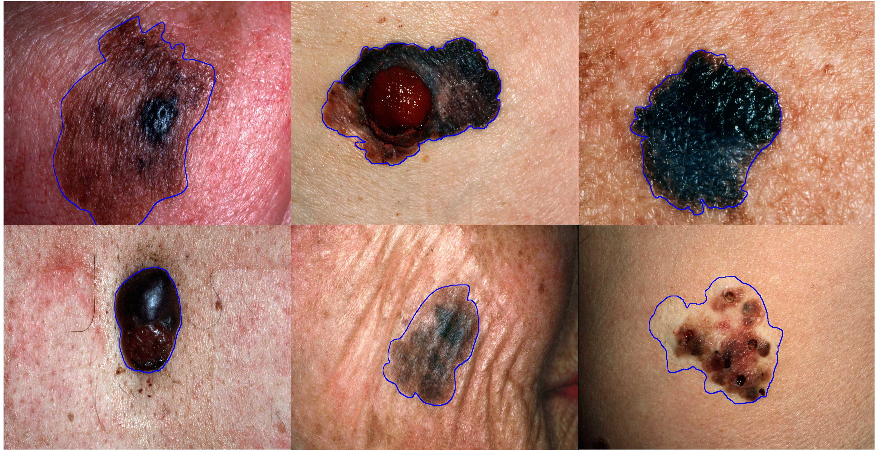
Image samples form DermQuest dataset.

Evaluation metrics

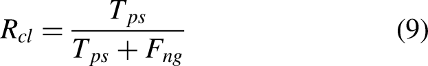
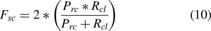
This part discusses the assessment criteria used and comprehensively analyzes the results. The most used metric for determining classification effectiveness is the classification’s accuracy (i.e., $A_{cr}$ ). It is calculated by dividing the number of images in the dataset by the number of occurrences (i.e., images) labeled correctly. In numerical form, it reads as follows, in equation (7):

$$Accuracy(A_{cr})=\frac{T_{ps}+T_{ng}}{T_{ps}+T_{ng}+F_{ps}+F_{ng}}$$

(7)

“True Positive” (i.e., $T_{ps}$ ) refers to the total number of verified melanoma images. False positive, abbreviated as $F_{ps}$ , refers to an incorrect tally of supposed false images. The percentage of melanoma images that were properly diagnosed as false negative (i.e., $F_{ng}$ ) vs. true negative (i.e., $T_{ng}$ ) is known as the “True negative” ( $T_{ng}$ ) count. It is the number of times a melanoma image was wrongly labeled as false. Precision (in our case $P_{rc}$ ) and recall (in our case $R_{cl}$ ) are standard metrics used to evaluate the effectiveness of image categorization algorithms. The $P_{rc}$ level is measured by how many images are correctly identified relative to the total number of images. $P_{rc}$ is expressed as a formula in equation (8):

$$P_{rc}=\frac{T_{ps}}{T_{ps}+F_{ps}}$$

(8)

$P_{rc}$ is important; however, $R_{cl}$ is equally crucial for assessing performance. In our case, $R_{cl}$ is the fraction of images that have been appropriately labeled relative to the total dataset images. Equation 9 represents the way to compute $R_{cl}$ value.

$$R_{cl}=\frac{T_{ps}}{T_{ps}+F_{ng}}$$

(9)

The harmonic mean of $R_{cl}$ and $P_{rc}$ is known as $F$ -score ( $F_{sc}$ ); the greater the value, the superior is system’s predictive ability. Therefore, it is not sufficient to evaluate the performance of a system based solely on its $P_{rc}$ or $R_{cl}$ . Equation 10 presents the F-score calculation.

$$F_{sc}=2*\left(\frac{P_{rc}*R_{cl}}{P_{rc}+R_{cl}}\right)$$

(10)

DermIS classification results

Accuracy

According to AlexNet, all experiments involving a color image from the necessary database should have an image size of 227 $\times$ 227 $\times$ 3. As a result, the needed image size is assumed to follow the required specifications. The ImageNet database classification is used for the convolutional network parameter. This proposed transfer learning model entirely automates feature extraction and classification processes. We optimized the model by altering several parameters. We looked at various training possibilities in order to get the best outcomes. We determined the optimal learning rate by changing numbers from le-1 to le-4. Similarly, using this optimal learning rate, we change the bias to achieve the best results and weight learns. Table 5 and Figure 12 show the classification results of the DERMIS dataset. When the proposed methodology is performed on the DERMIS dataset, it achieves 98.4% accuracy with a 1.6% error rate with Alexnet and 98.8% accuracy with a 1.2% error rate when compared to other algorithms (i.e., Almansour and Jaffar, ⁴³ Amelard et al., ⁷⁹ Bukhari et al., ⁸ Hosny and Kassem, ⁴ Jeyakumar et al., ²⁷ Khan et al., ⁷⁷ Mustafa et al., ¹⁹ and Shoieb et al., ⁷⁸ ), it shows 3%, 8%, 8%, 9%, 8%, 1%, 3%, and 1% more percentage difference, respectively, it has The average accuracy of 5% more (in both the cases) than the state-of-the-art.

Figure 12.

Accuracy percentage on DermIS dataset.

Table 5.

Classification results comparison for DermIS.

model	Classifier	Accuracy	Error rate
Proposed	CNN with Alexnet	98.4%	1.6%
Proposed	CNN with Densenet	98.8%	1.2%
Khan et al. 80	SVM	96%	4%
Shoieb et al. 78	SVM	94%	6%
Amelard et al. 79	SVM	94%	6%
Almansour and Jaffar 43	SVM	90%	10%
Hosny and Kassem 4	CNN	93.5%	6.5%
Bukhari et al. 8	CNN	97.4%	2.6%
Mustafa et al. 19	CNN	95.5%	4.5%
Jeyakumar et al. 27	CNN	97.6%	2.4%

CNN: convolutional neural network; SVM: support vector machine.

F1 score, precision, and recall

Table 6 and Figure 13 show the proposed model’s F1 score, precision, and recall values on the DermIS dataset. The efficacy of the proposed model is assessed with Alexnet and Densenet CNN models. Following fine-tuning, the model’s results for the selected parameters have improved for both the models. For instance, after tuning, the F1 score for Alexnet is 75.5, precision is 74, and recall is 77%. Whereas, Densenet shows more improvement than the Alexnet with 79.9%, 78%, and 82% more F1 Score, precision, and recall percentages. It indicates that the model’s performance has significantly improved after its optimized hyperparameters. In addition, changes in other parameters indicate that fine-tuning positively affects the model’s overall performance.

Figure 13.

Precision, recall, F1-Score for DermIS dataset.

Table 6.

Classification results comparison for DermIS.

Proposed model	F1 score	Precision	Recall
CNN with Alexnet	75.5	74	77
CNN with Densenet	79.9	78	82

DermQuest classification results

Accuracy

Similar to DermIS, we applied the same model to the DermQuest dataset. The classification findings of the DermQuest datasets are shown in Table 7. When the proposed technique is performed on the DermQuest datasets, it achieves 98.4% accuracy with a percentage of 1.6 error rate with Densenet and 97.2% accuracy with a percentage of 2.8 error rate with Alexnet. All other algorithms have little accuracy rate. It is to be noted that all these algorithms have used SVM and CNN-based classifiers.

Table 7.

Classification results comparison for DermQuest.

Models	Classifier	Accuracy	Error rate
Proposed	CNN with Alexnet	97.2%	2.8%
Proposed	CNN with Densenet	98.4%	1.6%
Hosny et al. 81	CNN	97.7%	2.3%
Naeem et al. 82	SVM	94.3%	5.7%
Khan et al. 83	SVM	94%	6%
Arasi et al. 41	CNN, DT	92.86%	7.14%
Hosny and Kassem 4	CNN	93.5%	6.5%
Bukhari et al. 8	CNN	94.7%	5.3%
Mustafa et al. 19	CNN	95.5%	4.5%
Jeyakumar et al. 27	CNN	97%	3%

SVM: support vector machine; CNN: convolutional neural network.

Figure 14 compares our model’s accuracy with state-of-the-art techniques. Compared to other algorithms (i.e., Arasi et al., ⁴¹ Bukhari et al., ⁸ Hosny et al., ⁸¹ Hosny and Kassem, ⁴ Jeyakumar et al. ²⁷ , Khan et al., ⁸³ Mustafa et al., ¹⁹ and Naeem et al., ⁸² ) there is 3%, 8%, 7%, 9%, 7%, 2%, 5%, and 8% more percentage difference, respectively. Comparing the proposed model to cutting-edge techniques reveals an average 6% improvement in accuracy (in both the cases).

Figure 14.

Accuracy percentage on DermQuest dataset.

F1 score, precision, and recall

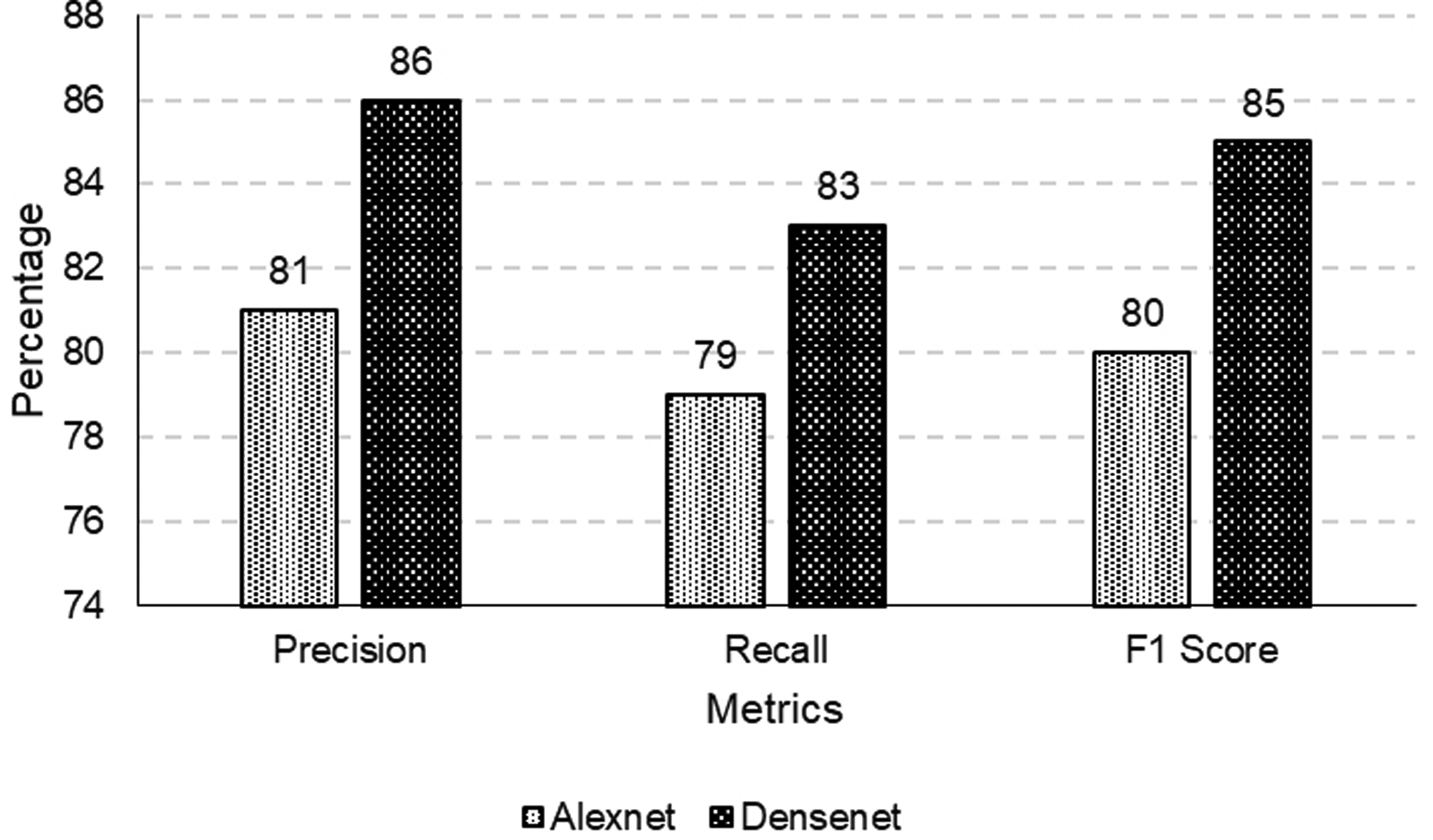
Table 8 and Figure 15 show the measurements of our proposed model’s F1 score, Precision, and Recall values on the DermQuest dataset. Our proposed model is evaluated using both Alexnet and Densenet models after fine-tuning. It is noted that the proposed model has gained better results in these parameters after tuning hyperparameters. After tuning the hyperparameters, the results obtained from the DermQuest dataset using our proposed model have significantly improved.

Figure 15.

Precision, recall, F1-Score for DermQuest dataset.

Table 8.

Classification results comparison for DermIS.

Algorithms	F1 Score	Precision	Recall
CNN with Alexnet	80	81	79
CNN with Densenet	85	86	83

After fine-tuning, the F1 score, which measures the model’s accuracy in balancing precision and recall, is 80% for the Alexnet and it is 85% in case of Densenet. It suggests our proposed model is more accurate at identifying melanoma cases in the DermQuest dataset using Densenet.

Similarly, the model’s precision, which measures the proportion of true positive results relative to all positive results, is 81 for the Alexnet and it is 86% for the Densenet after fine-tuning. It indicates a significant improvement in the model’s ability to correctly identify melanoma cases among all detected cases. In addition, recall, which measures the proportion of true positive results among all actual positive cases, is 79% for the Alexnet and it is 83% in case of Densenet, showing afficacy of Densenet over Alexnet.

Our model is better at overall classification accuracy and finding a balanced trade-off between correctly identifying malignant cases and minimizing false positives and negatives. However, it is important to note that the specific context of the dataset, its class distribution, and the potential consequences of misclassifications should be considered when interpreting these metrics and comparing models. Notably, the model’s efficacy depends on the training data’s quality, diversity, and representativeness. Imbalances and biases within the training dataset could lead to suboptimal generalization and susceptibility to overfitting. Augmentation strategies should be judiciously employed to ensure an inclusive representation of melanoma manifestations across diverse patient populations. Moreover, the model’s generalization to clinical scenarios necessitates validation across heterogeneous and real-world datasets, encompassing variations in image quality, lighting conditions, and patient profiles. The influence of transfer learning-induced biases demands scrutiny to ascertain that predictions remain equitable and unbiased across diverse populations. While our model has demonstrated commendable accomplishments, it is important to acknowledge several limitations that warrant attention for future research and development. One notable limitation pertains to the choice of the backbone architecture. In contrast, we know the advancements in image classification technology, including the emergence of image transformers. In light of this, we acknowledge the need to transition to a more performant backbone architecture in forthcoming contributions. Exploration of alternative architectures and enhancing model interpretability are promising avenues for future research. Techniques such as the utilization of gradient-based class activation maps hold the potential to offer transparency into model predictions, a factor of utmost significance for building trust among medical professionals.

ISIC2019 dataset classification results

To assess the performance of the proposed model on the ISIC2019 dataset, we initially deployed it on AlexNet and subsequently on DenseNet. We compared the results with the reference model presented in Olayah et al. ²⁸ The metrics used for the comparison are accuracy, F1 score, precision, and recall. They provide significant insights into the effectiveness of each framework with respect to our particular classification task. An initial comparison between AlexNet and DenseNet indicates that in every metric, both models surpass the performance of the reference model. This discovery emphasizes the progressions achieved in model architectures, demonstrating their efficacy in the domain of classification. Table 9 represents the comparison of different performance metrics for ISIC2019 dataset.

Table 9.

ISIC2019 dataset metrics comparison.

Metric	AlexNet	DenseNet	Olayah et al. 28	Percentage improvement in	Percentage improvement in
				DenseNet over Alexnet	DenseNet over 28
Accuracy	96.8%	97%	96.1%	0.73%	0.83%
F1 Score	98.4%	98.7%	96.9%	1.54%	0.65%
Precision	89.5%	90%	88.69%	0.91%	1.11%
Recall	91%	90.4%	89.5%	-1.68%	1.34%

It is worth mentioning that DenseNet consistently exhibits enhanced performance in comparison to AlexNet, as depicted in Figure 16. In terms of accuracy, F1 score, precision, and recall, DenseNet demonstrates superior performance, suggesting an enhanced ability to accurately classify instances while maintaining a more favorable trade-off between precision and recall. The obtained outcomes are consistent with the increasing recognition of DenseNet’s effectiveness in diverse image classification tasks as a result of its dense connectivity architecture. DenseNet, with an accuracy of 97%, demonstrates a superior ability to correctly classify instances compared to AlexNet, which achieved an accuracy of 96.8%. Moreover, the performance of DenseNet exceeds that of the reference model by 0.9%, affirming its efficacy in achieving superior accuracy. With an F1 score of 98.7%, DenseNet achieves a refined equilibrium between precision and recall compared to AlexNet’s F1 score of 98.4%. It signifies DenseNet’s superior performance in discerning intricate patterns within the dataset, resulting in a more robust and balanced classification model. Notably, DenseNet outperforms the reference model by 1.8%, affirming its effectiveness in achieving a precision of 90%. Whereas AlexNet has slightly higher recall (i.e., 91%), both models significantly surpass. ²⁸

Figure 16.

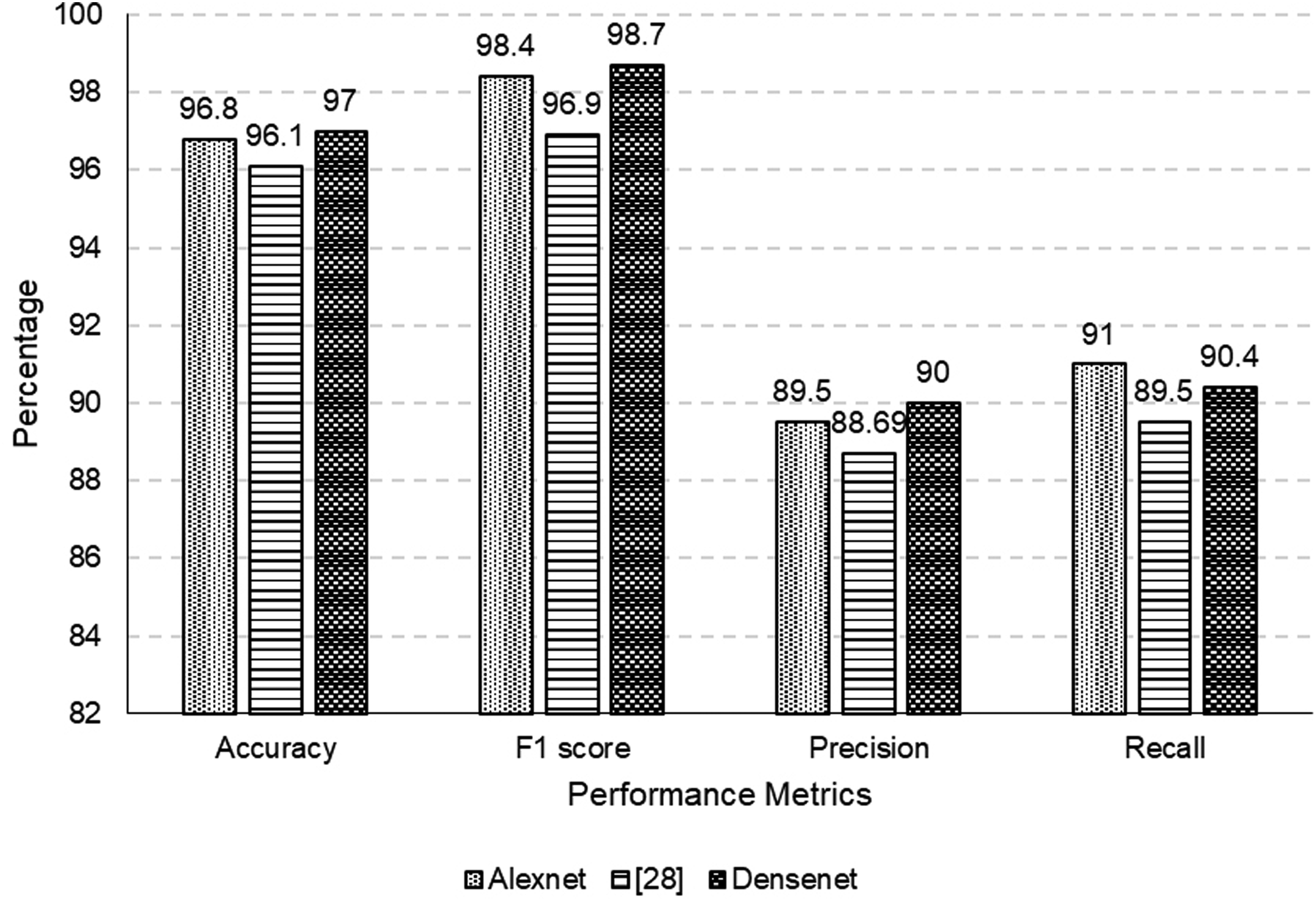
Accuracy, precision, recall, F1-Score for ISIC2019 dataset.

The percentage differences underscore the gradual enhancements achieved through the implementation of DenseNet, which manifests in significant improvements to accuracy, precision, and F1 score. Significantly, the performance of our suggested model is enhanced when executed on DenseNet in comparison to its execution on AlexNet. The noticeable percentage enhancements in accuracy, precision, and F1 score highlight the beneficial effects of implementing DenseNet within our particular framework. The results of this study indicate that the dense connectivity and feature reuse functionalities that are intrinsic to DenseNet make a substantial contribution to the model’s capacity to identify complex patterns in the dataset.

Conclusion and future work

Detecting melanoma is crucial for effective management, given its severity as a health concern. The utilization of AI and DL models, particularly CNN, has demonstrated encouraging outcomes in enhancing the Precision of melanoma categorization. We investigated refining a pre-existing AlexNet and densenet model to improve the efficacy of melanoma classification. The analysis shows that DenseNet outperforms AlexNet in the proposed image classification model. DenseNet’s accuracy and precision make it a more suitable choice for this task. By manipulating hyperparameters of the pre-existing model, we could attain an elevated level of accuracy in the classification of melanoma on the given datasets. The application of DL and machine learning methods in the classification of melanoma is an expanding area of research that holds promise for enhancing the detection and treatment of melanoma. The findings demonstrated that the fine-tuned model performed better than the pre-trained model, reaching high accuracy, F1 Score, Precision, and Recall. The model extracted the most critical characteristics from the input images with the help of CLs, ReLU, and response normalization layers. Optimizing DL models may significantly improve the effectiveness of melanoma classification systems. Nevertheless, additional investigation and verification on more extensive datasets are required to guarantee the Precision and dependability of these models. Future work will involve applying our model to larger datasets and incorporating more advanced DL techniques to enhance further the classification accuracy and efficacy of melanoma and other skin diseases. The availability of additional data may facilitate the development of more precise and tailored models for detecting and managing melanoma. Finally, it is imperative to carry out comprehensive clinical investigations to appraise the efficacy of these models in practical settings and evaluate their influence on patient results.