Sage Journals: Discover world-class research

Abstract

Objective

The introduction of new clinical risk scores (e.g. European System for Cardiac Operative Risk Evaluation (EuroSCORE) II) superseding original scores (e.g. EuroSCORE I) with different variable sets typically result in disparate datasets due to high levels of missingness for new score variables prior to time of adoption. Little is known about the use of ensemble learning to incorporate disparate data from legacy scores. We tested the hypothesised that Homogenenous and Heterogeneous Machine Learning (ML) ensembles will have better performance than ensembles of Dynamic Model Averaging (DMA) for combining knowledge from EuroSCORE I legacy data with EuroSCORE II data to predict cardiac surgery risk.

Methods

Using the National Adult Cardiac Surgery Audit dataset, we trained 12 different base learner models, based on two different variable sets from either EuroSCORE I (LogES) or EuroScore II (ES II), partitioned by the time of score adoption (1996–2016 or 2012–2016) and evaluated on holdout set (2017–2019). These base learner models were ensembled using nine different combinations of six ML algorithms to produce homogeneous or heterogeneous ensembles. Performance was assessed using a consensus metric.

Results

Xgboost homogenous ensemble (HE) was the highest performing model (clinical effectiveness metric (CEM) 0.725) with area under the curve (AUC) (0.8327; 95% confidence interval (CI) 0.8323–0.8329) followed by Random Forest HE (CEM 0.723; AUC 0.8325; 95%CI 0.8320–0.8326). Across different heterogenous ensembles, significantly better performance was obtained by combining siloed datasets across time (CEM 0.720) than building ensembles of either 1996–2011 (t-test adjusted, p = 1.67×10⁻⁶) or 2012–2019 (t-test adjusted, p = 1.35×10⁻¹⁹³) datasets alone.

Conclusions

Both homogenous and heterogenous ML ensembles performed significantly better than DMA ensemble of Bayesian Update models. Time-dependent ensemble combination of variables, having differing qualities according to time of score adoption, enabled previously siloed data to be combined, leading to increased power, clinical interpretability of variables and usage of data.

Keywords

Cardiac surgery risk prediction machine learning mortality ensemble learning dynamic model averaging legacy scores multi-modal data

Introduction

The European System for Cardiac Operative Risk Evaluation (EuroSCORE) I, also called Logistic EuroSCORE (LogES)¹ is a widely used Logistic Regression (LR) prediction tool in Europe and other parts of the world to estimate the risk of operative mortality following cardiac surgery.² This score was developed in 1999 using 19,030 patients collected over three months (September–December 1995) from 132 cardiac centres in eight countries.³ It uses a limited set of variables, such as age, sex, left ventricular ejection fraction (LVEF), and preoperative cardiac risk factors, to predict the risk of mortality. 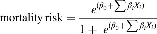However, lack of discrimination and calibration remains a problem in particular for high-risk patients.⁴ EuroSCORE (ES) II, is the more recent LR model developed in 2011 using data from 3 May to 25 July 2010.⁵ It uses a combination of patient demographics, medical history, and procedure-specific factors to predict the risk of in-hospital mortality.⁶ The logistic equation used was:

mortality risk = \frac{e^{(β_{0} + \sum β_{i} X_{i})}}{1 + e^{(β_{0} + \sum β_{i} X_{i})}}

ES II includes a more comprehensive set of variables than LogES, increased level of granularity for comorbidities like pulmonary hypertension, renal dysfunction, left ventricule dysfunction and information for the specific surgical procedures being performed, such as the number of procedures, the urgency of the procedures. ES II also includes a new comorbidity variable for diabetes and new symptom-based classification systems such as the New York Heart Association (NYHA) classification for assessing severity of heart failure^7–9 and the Canadian Cardiovascular Society classification system for severity of angina in patients with coronary artery disease.¹⁰ Although the ES II has been considered as a more accurate predictor of surgical risk, it no longer includes the post infarct septal rupture variable from LogES due to insufficient number of cases at the time of collection and missingness of newly included variables in periods before 2011 have not been well documented for cardiac centre data in the UK. ES II is more complex to calculate, less well known and less validated than LogES. Details of differences between the two scores are shown in Table 1.

Table 1.

LogES and ES II variables included in ML and Bayesian Update models.

LogES	LogES coefficient	ES II	ES II coefficient
Age (per 5 years over 60 years)	0.066	Age	0.0285181↓
Female gender	0.330	Female gender	0.2196434↓
Serum creatinine > 200 µmol/L	0.652	Renal impairment - On dialysis - CrCl ≤ 50 (severe) - CrCl 50–85 (moderate)	≡ 0.6421508 0.8592256 0.303553
Extracardiac arteriopathy	0.656	Extracardiac arteriopathy	0.5360268↓
Chronic pulmonary disease	0.493	Chronic pulmonary disease	0.1886564↓
Neurological dysfunction (poor mobility)	0.842	Neurological dysfunction (Poor mobility)	0.2407181↓
Previous cardiac surgery	1.003	Previous cardiac surgery	1.118599
Recent myocardial infarction	0.546	Recent myocardial infarction	0.1528943↓
Left ventricular ejection fraction (LVEF) - Moderate (30–50%) - Poor (<30%)	0.419 1.094	Left ventricular ejection fraction (LVEF) - Moderate (31–50%) - Poor (21–30%) - Very poor (≤20%)	≡ 0.3150652↓ 0.8084096 0.9346919
Systolic pulmonary pressure > 60 mmHg	0.768	Systolic pulmonary pressure - 31–55 mmHg - ≥ 55 mmHg	≡ 0.1788899 0.3491475↓
Active endocarditis	1.101	Active endocarditis	0.6194522↓
Unstable angina	0.568	CCS class 4 angina	0.2226147↓
Procedure urgency - Emergency	0.713	Procedure urgency - Urgent - Emergency - Salvage	≡ 0.3174673 0.7039121 1.362947
Critical preoperative state	0.906	Critical preoperative state	1.086517
Post infarct septal rupture	1.462	-
Other than isolated CABG	0.542	Weight of intervention - Single non-CABG - 2 Procedures - 3 Procedures	≡ 0.0062118 0.5521478 0.9724533
Surgery on thoracic aorta	1.160	Surgery on thoracic aorta	0.6527205↓
		NYHA - II - III - IV	0.1070545 0.2958358 0.5597929
		Diabetes on insulin	0.3542749
βo constant	4.789594		−5.324537

Bold variables in ES II that are substantially different to LogES; only non-baseline subcategories are shown; original score coefficients and constants before Bayesian Update are shown; these are not used for ML models; arrows show relative change in original coefficients: ES II versus LogES.

ES II has been shown by numerous studies to display poor discrimination and calibration across datasets with differing characteristics, including but not limited to age, ethnicity, time,¹¹ geographical locations¹¹ and procedures groups.^12–17 Preventing model miscalibration is critical in order to avoid ineffective treatment recommendations, harm to the patient¹⁸ and waste of scarce clinical resources.¹⁹

Ensemble models are a machine learning (ML) approach that combines two or more models in the prediction process and then synthesises the results into a single score or probability distribution to improve the accuracy of predictions. Some studies have assessed the performance of single ML algorithms (referred to as base learners in the ensemble context) against ES II and LR in small or medium-sized cohorts,^20,21 but have not considered Ensemble-based modelling approaches. This approach has the potential to reduce the amount of error in the prediction attributable to variance.²² Conversely, when a model's variance is high, it performs well on training data but inaccurately on test data (known as overfitting).

Currently, the vast majority of cardiac surgery risk stratification studies rely solely on the area under the curve (AUC) and only few studies have evaluated calibration, and clinical usefulness.^19,23–28 The AUC is not well suited for assessing cardiac outcomes with very low incidence rates, and typically mortality rates are as low as 3%. The No Free Lunch Theorem states that all optimisation algorithms perform equally well when their performance is averaged across all possible problems,²⁹ suggesting there is no best model, and that different models perform better under different data distributions. A key consideration in ensemble learning is achieving diversity from base learners. There are various ways to generate ensembles, and one approach is to combine using the same type of base learner (homogenous ensembles (HEs)), but with different samples of the data. Some ML classifiers are inherently HEs in nature such as the Random Forest (RF) and Xgboost models. The alternative is to consider a collection of diverse model types (heterogenous ensembles).

Dynamic model averaging (DMA) is a method for combining the predictions of multiple models in order to make more accurate predictions,^30,31 while ensemble learning is a more general framework that includes DMA as one of its many possible approaches. It involves continuously training and updating a set of models, and weighting their predictions based on their past performance. One framework for updating is to use Bayesian Updating,^30,32 which is a method of incorporating new information into an existing probability distribution, i.e. updating our prior beliefs about a hypothesis or parameter as new data or evidence becomes available. The process of updating is done through Bayes’ theorem, which states that:

P (H | D) = \frac{P (D | H) \cdot P (H)}{P (D)}

The posterior probability P(H|D) is calculated using the prior probability P(H) and the likelihood P(D|H) of the data given the hypothesis. The prior probability reflects our initial belief about the hypothesis before we have any data, and the likelihood reflects the fit of the data to the hypothesis. In the case of a Bayesian LR trained on LogES,³³ the prior is the original coefficients of the LogES model derived from the original LogES dataset before updating of the current dataset. The coefficients are typically adjusted using a latent algorithm that estimates or infers the data for variables through posterior sampling of observed data. One such algorithm is the Markov chain Monte Carlo (MCMC) simulation strategy for sampling from posterior probability distributions using Markov chains.³⁴ While DMA by Bayesian Updating is itself an ensemble approach, combining DMA for legacy risk scores such as LogES with updates scores such as ES II using ensemble method have yet to be considered.

Due to the late adoption of the ES II scoring system, the clinical recording of the 18 variables used to calculate this score began after year 2011, restricting the usage of these variables for modelling to the period 2012–2019. This makes it challenging to achieve full utilisation of the National Adult Cardiac Surgery Audit (NACSA) dataset, ranging from 1996 to 2019 for the purpose of risk stratification. While other variables within the range of 1996–2011 could be considered if missing rates are lower, the high usage of the most commonly considered scoring system, LogES,^35,36 within this time interval implies that its 17 variables would be suitable for risk stratification in terms of low missing rates and high clinical interpretability.

Under the assumption that ML models perform better when provided with larger datasets (Big Data), we combined siloed data in the periods 1996–2011 and 2012–2019 using ensemble models trained on logES and ES II variables, respectively. We hypothesised that Homogenenous and Heterogeneous ML ensembles will have better performance than ensembles of DMA for incorporating knowledge from LogES legacy data with ES II data to predict cardiac surgery risk. We proposed to consider both homogenous and heterogenous ensembles, as well as DMA as a special case of ensembles in the benchmarking process consensus metric (Figure 1).

Figure 1.

Design overview of the study; homogenous ensembles (logES-ESII-P) and heterogenous ensembles logES-O, ESII-O and logES-ESII-A were built and evaluated consensus metric. Further details of each model are provided in Supplemental materials. Mark Chain Monte-Carlo (MCMC) was used as the latent algorithm of Dynamic Model Averaging by Bayesian Update models; data were partitioned based on risk score adoption periods 1996–2016 (LogES) and 2012–2016 (ES II) and ensembled using the respective score variables; 2017–2019 data was used as hold-out data for evaluation.

Related works

We have previously evaluated the calibration changes in ML base models across the 1996–2011 and 2011–2017 for the EuroSCORE I variables and shown that both LR and RF models were associated with good discrimination ability but substantial miscalibration.³⁷ In a separate study, we have developed an approach that compared calibration changes, variable importance drift, performance drift and actual dataset drift of the base models using EuroSCORE II variables across the years 2017–2019. With respect to changes in techniques, Dataset drift was observed across the Holdout time periods for Weight of intervention. Sharp dataset drifts were observed for the Single non-CABG and 3 procedures category between 2018–12 and 2019–02. However, studies so far have either considered EuroSCORE I and EuroSCORE II in isolation,^38–41 with addition of new variables⁴² or have compared their performances side by side,^43–45 but have not considered the combination of the two scores. DMA has been suggested to be beneficial for model performance if applied to dynamically update more than one model in parallel.^30,31 According to a recent review, only a few studies have utilised and evaluated DMA approaches for clinical prediction models, with the majority focusing on discrete updating methods and model generalisability across populations rather than ways to handle temporal changes over time.³¹

While the vast majority of clinical studies rely solely on threshold-independent metrics such as the AUC, they have not evaluated cardiac risk models using consensus metrics (i.e. a combination of several metrics using approaches such as weighted arithmetic or geometric mean to improve robustness of performance evaluation).^19,23–28 Consensus metrics has been used to evaluate Covid-19 predictions,⁴⁶ and recently in our study using a consensus metric (clinical effectiveness metric (CEM)), with the latter study showing that ES II suffered from severe performance drift across multiple important performance metrics.⁴⁷ While ML approaches such as Xgboost and RF were more resistant to dataset and concept drift (drift in a model's decision boundary – sometimes measured indirectly through variable importance drift), these two models still showed performance decrease in at least 3 of the 5 performance metrics considered.⁴⁷ However, to our knowledge, consensus metrics have not yet been applied to evaluate ensemble models in cardiac surgical risk stratification.

Ensemble-model-based approaches to drift adaptation and preventing concept drifts have been described experimentally but also not been clinically applied.^48,49 With most of the ensemble models proposed in literature being homogeneous models, very few heterogeneous ensemble models have been proposed.⁵⁰ Even fewer studies have fully evaluated ML ensemble models that combine scores with substantially different levels of variable missingness across different time periods.^{19,26–28,51}

Materials and methods

The register-based cohort study is part of a research approved by the Health Research Authority and Health and Care Research Wales and a waiver for patients’ consent was waived (IRAS ID: 278171). An Abbreviations and Definitions list of frequently used technical terms used in this study has been provided for the reader at the start of the Supplemental materials.

Dataset and patient population

The study was performed using the NACSA dataset, which comprises UK adult cardiac surgery data prospectively collected by NACSA. Patients under the age of 18, having congenital cases, transplant and mechanical support device insertions and missing information on mortality were excluded. Rather than only examining the dataset across one institution as previously reported,³⁷ this analyses was performed using data for all NHS cardiac surgery hospital sites across the UK and a selection of private hospitals from 1 January 1996 to 31 March 2019.

Missing and erroneously inputted data in the dataset were cleaned according to the NACSA Registry Data Pre-processing recommendations; details are found in the Supplemental materials, Treatment of Missing Data section. The two sets of variable for LogES and ES II were included (Table 1). The LogES contained 17 variables, and we split the LVEF categories into two variables: Moderate (30–50%) and Poor (<30%) so that the input data is an 18-dimension vector per sample. The 18 variables of ES II were all included.

A total of 647,726 patients from 45 hospitals were included in this analysis following the removal of 4244 (0.65%) patients missing information on mortality.

We acknowledge that the techniques, risk profile and outcomes will have evolved over time. This is the inherent reason why prediction models need to be updated periodically. We have temporally split the data for three reasons. Primarily, this process mimics the natural development of prediction models with prospective verification of predictive ability following model development. Secondly, cohorting the training dataset by time effectively removes the bias of time-based variation in the predictor and outcome variables when developing the models (i.e. they are all equally effected by temporal changes). Thirdly, it allows one to review calibration drift as we have done in our previous work.⁵²

The dataset was split into three cohorts: Training 65% (n = 420,639; 1996–2011; Supplemental materials, Table S1), Update 24% (n = 157,196; 2012–2016; Table S2) and Holdout 11% (n = 69,891; 2017–2019; Table S3). The primary outcomes were discrimination, calibration, clinical utility and overall accuracy of the different models in prediction of in-hospital mortality risk following cardiac surgery.

Baseline statistical analysis

Continuous variables were measured with mean and standard deviation (SD). Categorical variables were described as frequency and percentage (%). Per pre-specified statistical plan, differences in baseline characteristics between the two groups were evaluated with Wilcoxon rank sum test for continuous variables, and Pearson's χ² test for categorical variables.⁵³

Scikit-learn v0.23.1 and Keras v2.4.0 were used to develop the models and to evaluate their discrimination capabilities. Statistical analyses were conducted using STATA-MP version 17 and R v4.0.2.⁵⁴ Anova Assumptions were checked using R rstatix package.

Preprocessing and linkage

A common id across both variable categories were created to ensure linkage. Data rows were then randomised using seed number 7 for reproducibility. Data standardization was performed by subtracting variable mean and dividing by the standard deviation values.⁵⁵

Geometric approach to ensemble learning and evaluation

The geometric mean is defined as $g (x, y) = \sqrt{x y}$ . Since $\log \sqrt{x y} = (\log x + \log y) / 2$ , the geometric mean can be interpreted as the antilog of the arithmetic mean of log transformed data. The Geometric mean is able to better adjust to outlier and small sized data than the arithmetic mean,⁵⁶ and does not ignore all data except the middle element as the median does. As we expect the different base learners of a small set of ensembles to have a skewed performance distribution in the probabilities predictions and evaluation scores, we select the Geometric mean as the function for (1) ensembling the base learner prediction probabilities; and (2) ensembling the set of M metrics used to evaluate the models.

DMA by Bayesian update

The Gibbs Sampling category of MCMC algorithm was used for the Bayesian update process by sampling from the posterior distribution of Bayesian models.^57,58 We applied a Bayesian LR model with variables and intercept coefficients latently sampled through MCMC. For the Bayesian Updated LogES base learners,³³ the prior was set as the original coefficients of the LogES model and latently updated using the 1996–2011 dataset. The updated coefficients were then used as priors for latently updating the coefficients using the 2012–2016 dataset. Due to late adoption of ES II, coefficients were updated using only data from 2012 to 2016 with the original ES II coefficients as priors. Three Chains of JAGs MCMC was applied, with each having 1000 iterations and burn-in of 200. Thinning interval was set to 10 and deviance information criterion was set to False. R2JAGS R package version 4.3.0 were used for Bayesian regression analysis.^59,60

Ensemble modelling

We used six statistical algorithms to generate mortality predictions – LR, Neural Network (Neuronetwork),⁵⁵ RF,⁶¹ Weighted Support Vector Machine (SVM),⁶² Xgboost⁶³ and DMA by Bayesian Update.^37,64 Each algorithm was ‘trained’ using two different sets of variables – those of LogES and ES II, such that the 12 Base learners were combined in different ways to build nine ensembles (Table 2).Geometric average was used for all soft-voting transformations to bring probability distribution of base learners into one ensemble distribution.⁶⁵ Details of base learner model specification are provided in Supplemental materials, Section 1.2. Training and Hyperparameter tuning settings for the base learner models are provided in Supplemental materials: Section 2 and Table S4.

Table 2.

Detailed specifications of the nine ensembles.

Model	Model category	Training variables	Model base learners	Training set	Update set	Holdout set
Bayesian Euroscore/Update Ensemble^a	logES-ESII-P (Homogeneous)	LogES variables	Bayesian updated LogES scores;	n = 420,639; (1996–2011)	n = 157,196; (2012–2016)	n = 69,891; (2017–2019)
Bayesian Euroscore/Update Ensemble^a	logES-ESII-P (Homogeneous)	ES II variables	Bayesian updated ES II scores		n = 157,196; (2012–2016)	n = 69,891; (2017–2019)
Logistic Regression (LR) Ensemble	logES-ESII-P (Homogeneous)	LogES variables	LR (LogES Base);	n = 577,835 (1996–2016)		n = 69,891; (2017–2019)
Logistic Regression (LR) Ensemble	logES-ESII-P (Homogeneous)	ES II variables	LR (ES II Base)		n = 157,196; (2012–2016)	n = 69,891; (2017–2019)
Random Forest (RF) Ensemble	logES-ESII-P (Homogeneous)	LogES variables	RF (LogES Base);	n = 577,835 (1996–2016)		n = 69,891; (2017–2019)
Random Forest (RF) Ensemble	logES-ESII-P (Homogeneous)	ES II variables	RF (ES II Base)		n = 157,196; (2012–2016)	n = 69,891; (2017–2019)
Neuronetwork (NN) Ensemble	logES-ESII-P (Homogeneous)	LogES variables	NN (LogES Base);	n = 577,835 (1996–2016)		n = 69,891; (2017–2019)
Neuronetwork (NN) Ensemble	logES-ESII-P (Homogeneous)	ES II variables	NN (ES II Base)		n = 157,196; (2012–2016)	n = 69,891; (2017–2019)
Xgboost Ensemble	logES-ESII-P (Homogeneous)	LogES variables	Xgboost (LogES Base);	n = 577,835 (1996–2016)		n = 69,891; (2017–2019)
Xgboost Ensemble	logES-ESII-P (Homogeneous)	ES II variables	Xgboost (ES II Base)		n = 157,196; (2012–2016)	n = 69,891; (2017–2019)
Weighted SVM Ensemble	logES-ESII-P (Homogeneous)	LogES variables	SVM (LogES Base);	n = 577,835 (1996–2016)		n = 69,891; (2017–2019)
Weighted SVM Ensemble	logES-ESII-P (Homogeneous)	ES II variables	SVM (ES II Base)		n = 157,196; (2012–2016)	n = 69,891; (2017–2019)
LogES-O Ensemble	logES-O (Heterogeneous)	LogES variables	LR (LogES Base); RF (LogES Base); NN (LogES Base); Xgboost (LogES Base); SVM (LogES Base);	n = 577,835 (1996–2016)		n = 69,891; (2017–2019)
ESII-O Ensemble	ESII-O (Heterogeneous)	ES II variables	LR (ES II Base); RF (ES II Base); NN (ES II Base); Xgboost (ES II Base); SVM (ES II Base);		n = 157,196; (2012–2016)	n = 69,891; (2017–2019)
logES-ESII-A Ensemble	logES-ESII-A (Heterogeneous)	LogES variables	LR (LogES Base); RF (LogES Base); NN (LogES Base); Xgboost (LogES Base); SVM (LogES Base);	n = 577,835 (1996–2016)		n = 69,891; (2017–2019)
logES-ESII-A Ensemble	logES-ESII-A (Heterogeneous)	ES II variables	LR (ES II Base); RF (ES II Base); NN (ES II Base); Xgboost (ES II Base); SVM (ES II Base);		n = 157,196; (2012–2016)	n = 69,891; (2017–2019)

This is Ensemble of DMA Bayesian Update combining LogES and ES II.

Ensemble models were created in two ways – heterogeneous or homogeneous techniques. Homogeneous models involve using the same algorithm to generate different models/predictions based on different temporal subsets of the base data (e.g. XGBoost based on ES II and XGBoost based on LogES variables), known as logES-ESII-P. Heterogeneous models involve using different algorithms on the same base data (e.g. XGBoost, LR, NN, RF … etc., all trained on ES II variables), known as logES-O, ESII-O and logES-ESII-A models. The ways for building the nine different ensembles are listed below:

A homogeneous Ensemble of DMA Bayesian Update models was built by using soft-voting to combine Bayesian updated LogES scores with Bayesian updated ES II scores.

The five other LogES base models were combined with ES II base models using soft-voting for each corresponding ML model pair, for example, RF (LogES) + RF (ES II).

The models above were all categorised as homogeneous logES-ESII Paired ensemble (logES-ESII-P). Heterogeneous models were also built and evaluated as follows:

An heterogeneous LogES only (logES-O) Ensemble is generated from the soft-averaging of all five LogES base ML models.

An heterogeneous ES II only (ESII-O) Ensemble is generated from the soft-averaging of all five ES II base ML models.

An heterogeneous logES-ESII Aggregate ensemble (logES-ESII-A) is generated from the soft-averaging of the logES-O and ESII-O ensembles.

It was not possible to cross-validate the ensembles built across variables from two unequal sized datasets n = 577,835 for LogES base learners and n = 157,196 for ES II base learners, since mismatch between validation set vectors’ probability length would not permit dot-product approaches to soft-voting. Instead, all models were evaluated using the Holdout dataset from the years 2017 to 2019 that were not part of the training process with performances compared to similar studies.⁶⁶

Assessment of model performance

The models’ performance was measured across four broad parameters, but based on a consensus metric approach as described later on in this section⁶⁷:

Discrimination: AUC,⁶⁸ F1 score⁶⁹

Calibration: 1−ECE.⁷⁰

Overall accuracy⁶⁷: 1−Brier score.⁷¹

Clinical utility: Net benefit analysis²⁰

The AUC performances of all variant models were evaluated, and the receiver operating characteristic (ROC) curves plotted.⁶⁸ The F _β score can provide an unbiased evaluation in imbalanced dataset scenarios, whereby the relative weighting of precision and recall are decided by the β parameter, with the F ₁ version being the most commonly used.⁶⁹ Decision curve net benefit index was used to test clinical benefit.²⁰ 1−Expected Calibration Error (ECE) was used to determine calibration performance, with higher values being better.⁷⁰ The adjusted Brier score (1−Brier) was used without the normalization term,⁷¹ but with higher values indicating higher overall accuracy performance.

To determine the best model in terms of both discrimination and calibration, we applied the consensus metric, CEM, which uses a geometric average^46,55,65 of AUC, F1,⁶⁹ decision curve net benefit (treated + untreated), 1−ECE and 1−Brier. 1000 bootstrap samples were taken for calculating all metrics. We then evaluated the following comparisons:

Ensemble of DMA Bayesian update models using LogES and ES II versus its base learners versus original LogES and ES II coefficient models.

logES-ESII-P (paired homogeneous) ensemble models against each other.

logES-O, ESII-O against logES-ESII-A models.

The logES-ESII-A ensemble against logES-ESII-P ensemble models.

Due to the CEM being computationally costly to calculate, comparison (1) and (2) above were selected using ROC-AUC and 95% CI to identify high performing candidate models for inclusion in subsequent comparisons. CEM performances for comparisons (3) and (4) were tested using one-way analysis of variance (ANOVA) with Bonferroni corrected multiple pairwise paired t-tests to minimise the possibility of false positive findings. Normality assumptions for ANOVA were checked using Shapiro–Wilk test.⁷² A drill down analysis of individual metric results comprising the CEM was conducted for comparison (4).⁷³

Model interpretation

Forest plots (R version 4.0.2, packages: tidyverse and ggforestplot) were used for comparing the Bayesian Updated LogES base learner coefficients against original logES coefficients and for comparing Bayesian updated ES II base learner against original ES II coefficient model. We also adopted the SHapley Additive exPlanations (SHAP) for the highest performing model to investigate which variables contribute most to mortality risk prediction on the Holdout set.⁷⁴ This model provides both high accuracy and consistency in terms of explaining which variables are important.⁷⁵ SHAP was used to examine the overall importance ranking of variables and applied to specific variables for interaction analysis. Importance was reported in either log-odds or absolute importance magnitude.

Results

Patients characteristics

A total of 647,726 adult cardiac surgery patients over 18 years from 45 hospitals were included in this analysis, following the removal of 3930 congenital cases, 1586 transplant and mechanical support device insertion cases and 4244 patients missing information on mortality. There were 21,374 deaths (mortality rate of 3.30%). A patient flow consort diagram is shown in Supplemental materials, Figure S1. Missing rates of variables for both the logES and ES II were low except for left ventricular function, pulmonary hypertension/arterial pressure, poor mobility and creatinine (Figures S2 and S3). Missing variables were backfilled using other informative variables according to NACSA dataset cleaning protocol: https://www.nicor.org.uk/wp-content/uploads/2018/09/nacsacleaning10.3.pdf and then imputed to improve variable quality, after which there were no missing variable values.

DMA LogES and ES II models

The baselearner DMA by Bayesian Update of LogES model obtained an AUC of 0.815 (95%CI: 0.8148–0.8154) and significantly outperformed the original LogES coefficient model AUC of 0.799 (95%CI: 0.7988–0.7995). The baselearner DMA by Bayesian Update of ES II model obtained an AUC of 0.811 (95%CI: 0.8105–0.8112) and significantly outperformed the original ES II coefficient model AUC of 0.799 (95%CI: 0.7988–0.7995). Ensemble of DMA Bayesian Update combining LogES and ES II obtained an AUC of 0.820 (95%CI: 0.8196–0.8203) and significantly outperformed either of DMA LogES and DMA ES II base learners alone as well as original coefficient score models.

A diagnostic of the two DMAbase learner models: Bayesian updated LogES and Bayesian updated ES II scores of the ensemble DMA model (results shown in subsequent sections) showed that characteristics of some variables, but not others in the NACSA dataset, have diverged substantially from the dataset from which the LogES and ES II coefficients were originally derived (Figure 2(a)–(b)). The original LogES overestimated the risk in high risk patients relative its Bayesian Update model (Figure 2(c)). There was higher tendency of the ES II to underestimate risk (Figure 2(d)). Overall, ES II scores having better calibration and less calibration drift across dataset and time, in terms of distance between original and updated coefficients (Figure 2(e)–(f)).

Figure 2.

(a) LogES MCMC 2012–2016 kernel density plots showing distribution of coefficient estimate for 6 LogES coefficients; red dotted lines show original LogES values; coefficients updated based on coefficients estimated using 1996–2011 dataset as prior; three kernels for each coefficient represent the three chains of MCMC estimates; (b) ES II MCMC 2012–2016 kernel density plots showing distribution of coefficient estimate for 6 ES II coefficients; red dotted lines show original ES II values; three kernels for each coefficient represent the three chains of MCMC estimates; (c) Histogram of LogES values calculated for 2017–2019 dataset using coefficients estimated from 2012 to 2016, which was updated based on coefficients estimated using 1996–2011 dataset; red shows the estimated distribution; green shows distribution based on the original LogES coefficients; (d) Histogram of ES II values calculated for 2017–2019 dataset using coefficients estimated from 2012 to 2016; red shows the estimated distribution; green shows distribution based on the original ES II coefficients; (e) Forest plot of LogES MCMC estimated coefficients for each variable versus original LogES coefficients; MCMC coefficients were obtained using data from 2012 to 2016 and updated based on coefficients from 1996 to 2011; 95% CI are narrow and barely visible; (f) Forest plot of ES II MCMC estimated coefficients for each variable versus original ES II coefficients; MCMC coefficients were obtained using data from 2012 to 2016; 95% CI are narrow and barely visible.

Homogeneous (logES-ESII paired) ensembles

Within the category of HEs (Figure 3(a)), the Xgboost HE was the highest performing model in terms of AUC (0.8327; 95% confidence interval (CI) 0.8323–0.8329) followed by RF HE (0.8325; 95%CI 0.8320–0.8326). Overlapping confidence indicates that the evidence of a difference is weak. The next highest AUC model was LR HE, for which the AUC (0.8258; 95%CI 0.8254–0.8260) was significantly lower than that of Xgboost and RF HEs. Neural Network HE was the fourth highest AUC model (0.8246; 95%CI 0.8242–0.8248), which had similar performance to Weighted SVM HE (0.8245; 95%CI 0.8240–0.8247). The Bayesian update HE (0.8200; 95%CI 0.8196–0.8203) performed worst. More comprehensive CEM results for HEs are described in subsequent sections.

Figure 3.

(a) Homogenous Ensembles: 5 LogES models are combined with the 5 ES II models using soft-voting for each corresponding ML model pair, for example, RF (LogES) + RF (ES II); the Bayesian Update Ensemble was built by using soft-voting to combine Bayesian updated LogES scores with Bayesian updated ES II scores; (b) multiple pairwise paired t-test for logES-O, ESII-O and logES-ESII-A; (c) ROC-AUC performances of logES-O, ESII-O and logES-ESII-A models; (d) logES-ESII-A results are compared against each of the logES-ESII-P models using multiple pairwise paired t-tests.

Heterogeneous ensemble models (logES-O, ESII-O and logES-ESII-A)

No extreme outliers were found. The CEM scores was normally distributed for all three models, as assessed by Shapiro–Wilk's test (p > 0.05). There was strong evidence of a difference across the three models p < 0.0001 as tested by ANOVA (Table S5). There was a significant evidence of a difference across all pairwise paired t-tests (Figure 3(b)). logES-ESII-A (CEM 0.720) was significantly better overall compared to ESII-O (p = 1.67×10⁻⁶) and logES-O (p = 1.35×10⁻¹⁹³) (Table S6). This indicates that a more diverse set of base learners combining siloed datasets across time periods enhanced performance across heterogenous datasets. The magnitude of difference in CEM between logES-ESII-A and ESII-O was smaller compared to other groups of comparison (Table S6: t-statistic 5.04 versus 37.7 and 33.3).

As drill down analysis, the ROC-AUC plot shows that performance ranking matched that of CEM and was in the ascending order logES-O, ESII-O and logES-ESII-A (Figure 3(c)). logES-ESII-A (0.8314; 95%CI 0.831–0.8316) provided significantly better discrimination than ESII-O (0.8305; 95%CI 0.8302–0.8308). There was statistical significance that both logES-ESII-A and ESII-O outperformed logES-O (0.8173; 95%CI 0.8168–0.8175).

Heterogeneous (logES-ESII-A) versus homogeneous (logES-ESII-P) ensemble models

No extreme outliers were found. The CEM scores was normally distributed for all models except LR logES-ESII-P HE, as assessed by Shapiro–Wilk's test (p > 0.05). There was a significant difference across models p < 0.0001, except between three logES-ESII-P HEs: LR, NN and RF (Table S7 and Figure 3(e)). logES-ESII-A was superior to the logES-ESII-P HEs: Bayesian Update, NN, and Weighted SVM (p < 0.0001). However, HEs: Xgboost and RF significantly outperformed logES-ESII-A (p < 0.0001), with Xgboost HE having highest overall performance ranking. No statistically significant difference in CEM performance was found for logES-ESII-A against LR logES-ESII-P (p > 0.05), although CEM score was lower in the latter model. Overall CEM performance of both HEs: Xgboost and RF were significantly higher than that of LR HE as demonstrated by no 95% CI overlap.

As a drill down analysis, logES-ESII-A (AUC 0.8314) was found to provide better discrimination, with no 95% CI overlap, than LogES-ESII-P ensembles: Bayesian Update (0.820), Weighted SVM (0.8245), Neuronetwork (0.8246) and LR (0.8258). Top four clinical overall benefit models were logES-ESII-P ensembles: NN logES-ESII-P (0.891), LR (0.890), RF (0.890) and Xgboost (0.889). Since net benefit index was calculated as the arithmetic average of the overall net benefit as per our previous study,⁴⁷ on average across all possible thresholds of decision, the net benefit of Xgboost homogeneous ensemble (0.889) that combines data across (EuroSCORE I variables, 1996–2011) and (EuroSCORE II variables, 2012–2016) was 0.079 higher than the Bayesian Update homogeneous ensemble (0.810). This equates to a net benefit of 790 per 10,000 patients. It was difficult to determine which model performed best across all metrics by examining each metric individually. However, the consensus metric CEM showed the overall ranking of model performances across all metrics (Table 3), which concorded with the multiple pairwise statistical tests. A detailed report of individual metric results comprising the CEM is given in Supplemental materials, Section 4.

Table 3.

Geometric mean of individual metrics for logES-ESII-A versus logES-ESII-P comparison.

Model category	ECE	AUC	Brier	F1	Net benefit	CEM.Mean	CEM.sd	CEM.CI lower limit	CEM.CI upper limit
Bayesian Update logES-ESII-P	0.935	0.820	0.970	0.268	0.810	0.694	0.005	0.694	0.695
logES-ESII-A	0.983	0.832	0.976	0.276	0.877	0.720	0.005	0.719	0.720
LR logES-ESII-P	0.996	0.826	0.976	0.269	0.890	0.719	0.005	0.719	0.719
NN logES-ESII-P	0.996	0.824	0.976	0.268	0.891	0.718	0.005	0.718	0.719
RF logES-ESII-P	0.994	0.832	0.976	0.275	0.890	0.723	0.005	0.723	0.723
Weighted SVM logES-ESII-P	0.798	0.825	0.927	0.263	0.520	0.608	0.005	0.608	0.609
Xgboost logES-ESII-P	0.993	0.832	0.976	0.279	0.889	0.725	0.005	0.725	0.725

CEM refs to clinical effectiveness metric; standard deviation and 95% CI are shown for CEM; adjusted 1−ECE and 1−Brier score values are shown; net benefit is average absolute overall benefit across all thresholds.

SHAP results

SHAP analysis was performed for Xgboost (ES II Base learner) on the Holdout set as the Xgboost HE was the best performing model. Most patients with important variables showed a clear separation of high variable values contributing to higher log-odds of mortality, and lower variable values contribute to lower log-odds (Figure 4(a)).

Figure 4.

(a) Tree SHAP feature importance plot for Holdout (n = 69,891; 2017–2019); every patient is represented as a dot; the x position of the dot is the impact of that feature on the model's prediction for that patient in log-odds; red: high variable values; blue: low variable values; patients that do not fit on the row pile up to show regions of high case volume; (b) mean absolute magnitude of importance across all prediction outputs; (c) log-odds of mortality (y-axis) versus normalised New York Heart Association (NYHA) Functional Classification values (x-axis); interactions of Operative Urgency are colored with red having higher normalised urgency; four vertical streaks from left to right show NYHA Classes: I, II, III, IV; (d) log-odds of mortality (y-axis) versus normalised renal impairment (x-axis); interactions with weight of intervention are colored with red having higher number of normalised procedures; four vertical streaks from left to right show renal impairment statuses: normal, moderate, on dialysis, severe.

An exception was renal impairment, which showed that patients with high pre-operative impairment can be associated with both high and low log-odds of mortality. The variables most associated with the prediction of mortality outcome were in decreasing order: weight of intervention, operative urgency, age, NYHA class, renal impairment, previous cardiac surgery, chronic pulmonary disease, extra-cardiac arteriopathy (peripheral vascular disease), critical preoperative state (Figure 4(b)). NYHA class III and IV, but not I and II were found to be associated with high log-odds of mortality (Figure 4(c)). Less urgent cases appear to be associated with higher log-odds of mortality for NYHA class II and III patients. Protective effect of dialysis was observed for patients with renal impairment (Figure 4(d)). Moderate renal impairment was associated with a low log-odds of mortality. Severe renal impairment was associated with high log-odds of mortality but was protected by increasing the number of procedures used in each operation.

Discussion

Pre-operative risk stratification based on ML has the potential to provide early risk identification and quantitative measures to assist physicians, patients, and family members in making critical surgical decisions, with increased individual specificity and accuracy compared to traditional models.^76–78 Identification of the best model, even in scenarios where there are only small differences in model performance is important for assessing fitness for surgery and deciding between surgical or non-surgical interventions.²³ Conversely, poor selection of models may lead to detrimental effects on patients outcome and hospital resource utilisation.

The aim of this study was to address the bias from the use of only EuroSCORE II variables that are only available in the period 2012–2019. Due to high missingness rates, the models cannot be built for the periods relating to 1996–2011 for models using EuroSCORE II (ES II). Hence, to minimise bias of considering only data in the 2012–2019 period, homogeneous ensembles such as the logES-ESII-P enabled complete coverage of the periods from 1996 to 2016 when making predictions or decisions on new data from 2017 to 2019. ESII-O Ensemble was the only model that did not incorporate knowledge from 1996 to 2011. We have included this model to understand whether the addition of historical data have the potential to add clinical predictive value to more recent data or such an approach is unnecessary given improvements through ensemble modelling of ES II variables. This would not have been comparable if models were not built for different eras. Hence, unlike our previous studies that evaluate the capabilities of the algorithms (albeit different models) considered here,^47,52 this study also compares the prediction performances of models built using varying amounts of data, that would have been siloed and unavailable if ensemble (or similar) approaches such as ones considered here were not applied.

In this study, we found that combining the metrics covering all four aspects of discrimination, calibration, clinical usefulness and overall accuracy into a single CEM improved the efficiency of cognitive decision-making (according to Miller's Law⁷⁹ for selecting the optimal ensemble models. While AUC does evaluate diagnostic or predictive performance of the model, it does not directly reflect patient benefit. This is why we have included a suit of other metrics including the Decision Curve net benefit index.

Furthermore, ML ensemble models performed significantly better than DMA of Bayesian Update models, which traditionally has been one of the few limited approaches for dealing with model miscalibration over time. We also drilled down and reviewed clinical utility using decision curve net benefit and found that the XGBoost homogeneous ensemble would result in many more patients being appropriately offered surgery as compared to the Bayesian Update homogeneous ensemble. Given that the mortality rate was low (3.3%), seemingly small statistically significant improvements may also be of clinical significance. This corroborated with previous findings.^20,52

Whilst Bayesian Update models enable useful visualisation of calibration drift across dataset and time, such models are very computationally inefficient for large datasets, whilst other ML ensembles have been found to be more efficient here.

This study also found that Xgboost/RF homogenous ensembling or a highly heterogeneous ensemble approach such as logES-ESII-A should be the preferred choice for high performance across multifaceted aspects of ML performance. Through the separate use of LogES and ES II variable sets in base learner models for both homogeneous and highly heterogeneous ensembles, the previously siloed data could be combined, leading to increased power, clinical interpretability of variables and usage of data. That is, the entire dataset ranging from 1996 to 2016 can be used for training, whilst this is not possible for the ES II category of models due to lack of data for periods before or near its adoption, that is, 1996–2011. Using conventional approaches, one would have to either use the lower performance LogES score, compromise by using a non-complete dataset using ES II or use computationally expensive Bayesian updating.^80–82

The inclusion of high-performing and more diverse models such as Neural Network, and Xgboost may have contributed to the reduction of high variance and bias issues, which could potentially be detrimental to discrimination, calibration, clinical utility and overall accuracy across datasets and time.^66,83 For example, the logES-ESII-A ensemble substantially exceeded the performance reported in a small sized study that used an ensemble of GBM, RF, support vector machine and Naïve Bayes, built using logES, ESII and other clinical variables without temporal consideration of variables, to predict cardiac postoperative mortality (AUC = 0.832 vs 0.795).²⁰ However, a smaller sized study that included Xgboost as part of a heterogeneous set of Super Learner ensemble did not achieve high performance using pre-operative data compared to this study's logES-ESII-A ensemble (AUC = 0.832 vs 0.718 [0.687–0.749]),⁸⁴ or homogeneous Xgboost and RF (logES-ESII-P) ensembles (AUC = 0.832). In addition, HEs: Xgboost and RF (AUC = 0.832) both outperformed the RF model reported (variables n = 46: 0.828, variable n = 8: 0.782) in a similar-sized study predicting mortality outcomes in heart failure patients.⁸⁵ The current study provides evidence supporting the use of the ensemble approaches described here for cardiac surgery mortality risk prediction.

Our study also shows that the base learner of the best performing Xgboost HE model can provide a detailed understanding of variable association to outcome for its parent ensemble model through the use of interpretive tools such as SHAP. This approach enables the analysis of not only variable importance and associations but also variable interactions.⁸⁶ The latter is not easily interpretable using the standard Bayesian Update approach.^{25,69,87–89} However, the inclusion of the Bayesian Update model, as part of an ensemble, has demonstrated improvement in interpretability of calibration drift for ensemble models in relation to the coefficients of the data on which they were originally modelled. The benefit of the SHAP approach over traditional LR is that both the individual patient procedural contribution to each variable's importance and the global variable importance in relation to the outcome can be simultaneously visualised. Since our models utilise a weighted average with equal weights for combining the models, one could also combine the variables’ importance using a weighted average or other user defined functions to observe the variable importance changes across combined models and periods of interests.

Limitations and future studies

This study is not without limitations. The study has limited variables available in the dataset. No medication specific variables were available in the national dataset for adjustment despite usage before and after cardiac surgery, but local and multi-centred collection efforts should be undertaken to further incorporate such information. We acknowledge that detailed procedures may not be captured by the variables considered within the two types of scores considered here within. Hence, future studies should explore the potential of adding additional detailed procedural information within the scores considered. In this regard, we have conducted pilot studies on the evaluation of procedural specific models using variables beyond ones considered here and found considerable variation of across models for individual procedures in the year 2017–2019. Furthermore, risk factors in addition to the EuroSCORE I and EuroSCORE II variables should be considered through variable selection approaches incorporating a wider set of candidate risk factors. In order to consider the full extent of variations in variable importance drift,⁴⁷ dataset drift, and performance drift, whereby numerous models are present in the same time period, future work may combine the corresponding variable importances of models using, e.g. weighted averages for comparison to other drift metrics.

Generalisability is an important topic that should follow in future studies using datasets from other populations or domains. For example, a similar ensemble-based dataset combination analysis should be conducted for the paediatric dataset for the PRAIS I⁹⁰ and PRAIS II⁹¹ scores. In addition, this approach could also be used to assess model performances combining risk scores and data from other outcome measures, for example, post-operative stroke, or other health conditions such as musculoskeletal disease or oncology.

Data on structural and functional abnormalities of the heart was also limited due to the lack of medical imaging data.⁹² Given the massive structural information medical images contain regarding the heart, we shall extract Echocardiography (Echo) features to test if the ranking of ensemble algorithm combinations identified here will be consistent when combining LogES and ES II variables with Echo data. Model combination approaches other than soft-voting such as data fusion,⁹³ Mixture of Experts,^94,95 SuperLearners⁹⁶ and diversity enhancement⁹⁷ transform of probabilities have not been considered here, but will be of interest in future studies. It would also be interesting to apply similar ensemble benchmarking approaches to identify the suitable models to use for combining variables and data from new cardiac interventions (e.g. TAVR⁹⁸ with that of historical interventions (SAVR) through clustering⁹⁹ and trajectory-based approaches.^100–102

A question that should be addressed is how to prevent large number of variables from decreasing the usability of the models. We envisage that future work will be to automate the extraction of variables from routinely collected databases in scenarios where the number of variables required for a model is larger than the clinician is willing to fill in. In such scenarios, it is envisaged that a report or form will be automatically filled in for the clinician through, for example, automated reporting dashboard. Our previous work on Covid-19 demonstrated that a much larger set of variables can be readily analysed and presented in clinically meaningful ways on a dashboard.¹⁰³ In addition, a much larger number of variables are considered by Diagnostic lab scientists when clinicians are informed on genetic abnormality results, so perhaps a future direction may involve the training more clinical scientists to support the clinicians in the interpretation of Big Data related models.

Conclusion

This study based on a large national registry data found that combining the metrics covering all four aspects of discrimination, calibration, clinical usefulness and overall accuracy into a single consensus metric improved the efficiency of cognitive decision-making for cardiac surgery risk model selection. The evaluation approach showed that Ensemble ML models outperformed the approach of ensemble of DMA Bayesian Update models. Xgboost/RF homogenous ensembling and a highly heterogeneous ensemble approach demonstrated high performance across multifaceted aspects of ML performance. It was shown that the time-dependent ensemble combination of variables, having differing quality according time of score adoption, enabled previously siloed data to be combined, leading to increased power, clinical interpretability of variables and usage of data. Lastly, it highlights the versatility of the SHAP tool for not only understanding why predictions are made by base learners of ensembles, but also the associations and interactions between variables and outcomes at both the individual and global levels. Future studies should aim to investigate ensemble approaches adjusting for score adoption to other cardiac surgery cohorts with different characteristics and explore whether other combinations of ensemble models can lead to further performance improvements.

Supplemental Material

sj-docx-1-dhj-10.1177_20552076231187605 - Supplemental material for Cardiac surgery risk prediction using ensemble machine learning to incorporate legacy risk scores: A benchmarking study

Supplemental material, sj-docx-1-dhj-10.1177_20552076231187605 for Cardiac surgery risk prediction using ensemble machine learning to incorporate legacy risk scores: A benchmarking study by Tim Dong, Shubhra Sinha, Ben Zhai, Daniel P Fudulu, Jeremy Chan, Pradeep Narayan, Andy Judge, Massimo Caputo, Arnaldo Dimagli, Umberto Benedetto and Gianni D Angelini in DIGITAL HEALTH

Footnotes

Acknowledgements

We are grateful to Hunaid A Vohra, Marco Gemelli, Lauren Dixon and Chris Holmes for comments on the draft of the manuscript.

Data availability

All data used in this study are from the National Adult Cardiac Surgery Audit (NACSA) dataset. These data may be requested from Healthcare Quality Improvement Partnership (HQIP), https://www.hqip.org.uk/national-programmes/accessing-ncapop-data/#.Ys6gN-zMLdp. Code for deriving training, update, and hold-out datasets is available on GitHub and authors can provide confirmatory de-identified record IDs for each set upon reasonable request.

Contributorship

TD, SS, AD, DPF, JC, BZ, PN, UB, AJ, and GDA contributed to experimental design. TD and SS acquired data. TD and SS performed the data preprocessing. TD wrote the source code to perform the experiments, and are accountable for all aspects of the work. TD, SS, AD, DPF, JC, BZ, PN, AJ, and GDA analyzed the results. TD wrote the first version of the paper. All authors revised the paper and approved the submission.

Code availability

All source code used in this study are available on GitHub (). Analyses were performed using Scikit-learn v0.23.1, Keras v2.4.0, STATA-MP version 17 and R v4.0.2.

Declaration of Conflicting Interests

The author(s) declared no potential conflicts of interest with respect to the research, authorship, and/or publication of this article.

Ethical approval

The study was approved by the Health Research Authority (HRA) and Health and Care Research Wales (HCRW) in 23 of July 2019, IRAS project ID: 257758 and a waiver for patients’ consent was obtained.

Funding

The author(s) disclosed receipt of the following financial support for the research, authorship, and/or publication of this article: This work was supported by a grant from the BHF-Turing Institute and the NIHR Biomedical Research Centre at University Hospitals Bristol and Weston NHS Foundation Trust and the University of Bristol.

Guarantor

ORCID iD

Tim Dong

Supplemental material

Supplemental material for this article is available online.

References

Nashef

SAM

Roques

Michel

, et al. European system for cardiac operative risk evaluation (EuroSCORE). Eur J Cardiothorac Surg 1999; 16: 9–13.

Holmes

Patel

, et al. Comparison of EuroSCORE II, original EuroSCORE, and the society of thoracic surgeons risk score in cardiac surgery patients. Ann Thorac Surg 2016; 102: 573–579.

Roques

Nashef

SAM

Michel

, et al. Risk factors and outcome in European cardiac surgery: analysis of the EuroSCORE multinational database of 19030 patients. Eur J Cardiothorac Surg 1999; 15: 816–823.

Gummert

Funkat

Osswald

, et al. EuroSCORE overestimates the risk of cardiac surgery: results from the national registry of the German society of thoracic and cardiovascular surgery. Clin Res Cardiol 2009; 98: 363–369.

Nashef

SAM

Roques

Sharples

, et al. EuroSCORE II. Eur J Cardiothorac Surg 2012; 41: 734–745.

Nezic

. Is it appropriate to use EuroSCORE II for prediction of 30-day mortality in cardiac surgery? Eur J Cardiothorac Surg 2021; 60: 34.

Miller-Davis

Marden

Leidy

. The New York Heart Association Classes and functional status: what are we really measuring? Heart Lung 2006; 35: 217–224.

Bredy

Ministeri

Kempny

, et al. New York Heart Association (NYHA) classification in adults with congenital heart disease: relation to objective measures of exercise and outcome. European Heart Journal - Quality of Care and Clinical Outcomes 2018; 4: 51–58.

Bennett

Riegel

Bittner

, et al. Validity and reliability of the NYHA classes for measuring research outcomes in patients with cardiac disease. Heart Lung 2002; 31: 262–270.

10.

Kotajärvi

Tolppanen

A-M

Hartikainen

, et al. Correlation of the disease-specific Canadian Cardiovascular Society (CCS) classification and health-related quality of life (15D) in coronary artery disease patients. PLOS ONE 2022; 17: e0266101.

11.

Sinha

Dimagli

Dixon

, et al. Systematic review and meta-analysis of mortality risk prediction models in adult cardiac surgery. Interact Cardiovasc Thorac Surg 2021; 33: 673–686.

12.

Silaschi

Conradi

Seiffert

, et al. Predicting risk in transcatheter aortic valve implantation: comparative analysis of EuroSCORE II and established risk stratification tools. Thorac Cardiovasc Surg 2015; 63: 472–478.

13.

Carnero-Alcázar

Silva Guisasola

Reguillo Lacruz

, et al. Validation of EuroSCORE II on a single-centre 3800 patient cohort. Interact Cardiovasc Thorac Surg 2013; 16: 293–300.

14.

Zhang

Wang

, et al. Validation of EuroSCORE II in Chinese patients undergoing heart valve surgery. Heart, Lung and Circulation 2013; 22: 606–611.

15.

Arangalage

Cimadevilla

Alkhoder

, et al. Agreement between the new EuroSCORE II, the Logistic EuroSCORE and the Society of Thoracic Surgeons score: implications for transcatheter aortic valve implantation. Arch Cardiovasc Dis 2014; 107: 353–360.

16.

Atashi

Amini

Tashnizi

, et al. External validation of European system for cardiac operative risk evaluation II (EuroSCORE II) for risk prioritization in an Iranian population. Braz J Cardiovasc Surg 2018; 33: 40–46.

17.

Provenchère

Chevalier

Ghodbane

, et al.

Is the EuroSCORE II reliable to estimate operative mortality among octogenarians?

PLOS ONE 2017; 12: e0187056.

18.

Van Calster

McLernon

van Smeden

, et al. Calibration: the Achilles heel of predictive analytics. BMC Med 2019; 17: 30.

19.

Davis

Lasko

Chen

, et al. Calibration drift among regression and machine learning models for hospital mortality. AMIA Annu Symp Proc 2018; 2017: 625–634.

20.

Allyn

Allou

Augustin

, et al. A comparison of a machine learning model with EuroSCORE II in predicting mortality after elective cardiac surgery: a decision curve analysis. PLOS ONE 2017; 12: e0169772.

21.

Mejia

OAV

Antunes

Goncharov

, et al. Predictive performance of six mortality risk scores and the development of a novel model in a prospective cohort of patients undergoing valve surgery secondary to rheumatic fever. PLoS One 2018; 13: e0199277.

22.

Ensemble Machine Learning . https://link.springer.com/book/10.1007/978-1-4419-9326-7 (accessed 18 Jul 2022).

23.

Nilsson

Algotsson

Höglund

, et al. Comparison of 19 pre-operative risk stratification models in open-heart surgery. Eur Heart J 2006; 27: 867–874.

24.

Walsh

Sharman

Hripcsak

. Beyond discrimination: a comparison of calibration methods and clinical usefulness of predictive models of readmission risk. J Biomed Inform 2017; 76: 9–18.

25.

Davis

Goadrich

. The relationship between Precision-Recall and ROC curves. In: Proceedings of the 23rd international conference on Machine learning. New York, NY, USA: Association for Computing Machinery 2006. 233–40. doi:10.1145/1143844.1143874.

26.

Lapp

Bouamrane

M-M

Kavanagh

, et al. Evaluation of random forest and ensemble methods at predicting complications following cardiac surgery. In: Riaño

Wilk

ten Teije

(eds) Artificial intelligence in medicine. Cham: Springer International Publishing, 2019, pp.376–385. doi:10.1007/978-3-030-21642-9_48

27.

Fernandes

MPB

Armengol de la Hoz

Rangasamy

, et al. Machine learning models with preoperative risk factors and intraoperative hypotension parameters predict mortality after cardiac surgery. J Cardiothorac Vasc Anesth 2021; 35: 857–865.

28.

Marvao

Dawes

Howard

, et al. Artificial intelligence and the cardiologist: what you need to know for 2020. Heart 2020; 106: 399–400.

29.

Adam

Alexandropoulos

S-AN

Pardalos

, et al. No free lunch theorem: a review. In: Demetriou

Pardalos

(eds) Approximation and optimization : algorithms, complexity and applications. Cham: Springer International Publishing, 2019, pp.57–82. doi:10.1007/978-3-030-12767-1_5

30.

Hickey

Grant

Caiado

, et al. Dynamic prediction modeling approaches for cardiac surgery. Circul Cardiovasc Qual Outcomes 2013; 6: 649–658.

31.

Jenkins

Sperrin

Martin

, et al. Dynamic models to predict health outcomes: current status and methodological challenges. Diagnostic Prognostic Res 2018; 2: 23.

32.

Genest

Schervish

. Modeling expert judgments for Bayesian updating. Annals Stat 1985; 13: 1198–1212.

33.

O’Brien

Dunson

. Bayesian multivariate logistic regression. Biometrics 2004; 60: 739–746.

34.

Beck

S-K

. Bayesian updating of structural models and reliability using Markov chain Monte Carlo simulation. J Eng Mech 2002; 128: 380–391.

35.

Hickey

Grant

Murphy

, et al. Dynamic trends in cardiac surgery: why the logistic EuroSCORE is no longer suitable for contemporary cardiac surgery and implications for future risk models. Eur J Cardiothorac Surg 2013; 43: 1146–1152.

36.

Siregar

Groenwold

RHH

de Heer

, et al. Performance of the original EuroSCORE. Eur J Cardiothorac Surg 2012; 41: 746–754.

37.

Benedetto

Sinha

Lyon

, et al.

Can machine learning improve mortality prediction following cardiac surgery?

Eur J Cardiothorac Surg 2020; 58: 1130–1136.

38.

Chan

Dimagli

Dong

, et al. Trend and factors associated with multiple arterial revascularization in coronary artery bypass grafting in the UK. Eur J Cardiothorac Surg 2022; 62. doi:10.1093/ejcts/ezac284

39.

Fudulu

Dimagli

Sinha

, et al. Weekday and outcomes of elective cardiac surgery in the UK: a large retrospective database analysis. Eur J Cardiothorac Surg 2022; ezac038. doi:10.1093/ejcts/ezac038

40.

Benedetto

Dimagli

Gibbison

, et al. Disparity in clinical outcomes after cardiac surgery between private and public (NHS) payers in England. The Lancet Regional Health – Europe 2021; 1. doi:10.1016/j.lanepe.2020.100003

41.

Fudulu

Dimagli

Sinha

, et al. Impact of preoperative atrial fibrillation on in-hospital outcomes of coronary artery bypass grafting. Semin Thorac Cardiovasc Surg Published Online First: July 2022. doi:10.1053/j.semtcvs.2022.07.002

42.

Belyaev

Skopin

Lobacheva

, et al. The combination of Euroscore II with a new variable ‘Nongraftable coronary artery lesions’ improves the discriminating power of the test in surgical patients with postinfarction ventricular septal defect and ventricular aneurysm. J Card Surg 2022; 37: 4952–4961.

43.

Spiliopoulos

Bagiatis

Deutsch

, et al. Performance of EuroSCORE II compared to EuroSCORE I in predicting operative and mid-term mortality of patients from a single center after combined coronary artery bypass grafting and aortic valve replacement. Gen Thorac Cardiovasc Surg 2014; 62: 103–111.

44.

Guillet

Moury

Bedague

, et al. Comparison of the additive, logistic European System for Cardiac Operative Risk (EuroSCORE) with the EuroSCORE 2 to predict mortality in high-risk cardiac surgery. Ann Card Anaesth 2020; 23: 277–282.

45.

Pascual

Palau Martí

Pajares

, et al. Preoperative risk assessment in cardiac surgery. EuroSCORE I and EuroSCORE II in a modern cohort. J Cardiothorac Vasc Anesth 2022; 36: 42.

46.

Devaraj

Madurai Elavarasan

Pugazhendhi

, et al.

Forecasting of COVID-19 cases using deep learning models: is it reliable and practically significant?

Results Phys 2021; 21: 103817.

47.

Dong

Sinha

Zhai

, et al. Performance drift is a major barrier to the safe use of machine learning in cardiac surgery. MedRxiv 2023. 2023.01.21.23284795. doi:10.1101/2023.01.21.23284795

48.

Liu

Zhang

. Diverse instance-weighting ensemble based on region drift disagreement for concept drift adaptation. IEEE Trans Neural Netw Learn Syst 2021; 32: 293–307.

49.

Krittanawong

Virk

HUH

Bangalore

, et al. Machine learning prediction in cardiovascular diseases: a meta-analysis. Sci Rep 2020; 10: 16057.

50.

Haque

Noman

Berretta

, et al. Optimising weights for heterogeneous ensemble of classifiers with differential evolution. In: 2016 IEEE Congress on Evolutionary Computation (CEC). 2016. 233–40. doi:10.1109/CEC.2016.7743800.

51.

Friedrich

Groß

König

, et al. Applications of artificial intelligence/machine learning approaches in cardiovascular medicine: a systematic review with recommendations. Eur Heart J - Digit Health 2021; 2: 424–436.

52.

Sinha

Dong

Dimagli

, et al. Comparison of machine learning techniques in prediction of mortality following cardiac surgery: analysis of over 220,000 patients from a Large National Database. Eur J Cardio-Thoracic Surg: Off J Eur Assoc Cardio-Thoracic Surg 2023. Published Online First: 5 August 2023. doi:10.1093/ejcts/ezad183

53.

Chan

Dimagli

Fudulu

, et al. On- versus off-pump CABG in octogenarians: a propensity-matched analysis from the UK national database. J Card Surg 2022; 37: n/a–n/a.

54.

StataCorp. Stata Statistical Software: Release 17. College Station, TX: StataCorp LLC; 2021.

55.

Dong

Benedetto

Sinha

, et al. A Deep Recurrent Reinforced Learning model to compare the efficacy of targeted local vs. national measures on the spread of COVID-19 in the UK. medRxiv Published Online First: 2021. doi:10.1101/2021.05.21.20248630

56.

Olivier

Johnson

Marshall

. The logarithmic transformation and the geometric mean in reporting experimental IgE results: what are they and when and why to use them? Ann Allergy Asthma Immunol 2008; 100: 333–337.

57.

Benedetto

Dimagli

Sinha

, et al. Machine learning improves mortality risk prediction after cardiac surgery: Systematic review and meta-analysis. J Thorac Cardiovasc Surg. Published Online First: 10 August 2020. doi:10.1016/j.jtcvs.2020.07.105

58.

Gelfand

. Gibbs sampling. J Am Stat Assoc 2000; 95: 1300–1304.

59.

Yoo

Chun

Hong

, et al. Risk prediction of three different subtypes of highly pathogenic avian influenza outbreaks in poultry farms: based on spatial characteristics of infected premises in South Korea. Front Vet Sci 2022; 9: 897763.

60.

Zhan

Jiao

Man

, et al. Using JAGS for Bayesian cognitive diagnosis modeling: a tutorial. J Educ Behav Stat 2019; 44: 473–503.

61.

Sarica

Cerasa

Quattrone

. Random forest algorithm for the classification of neuroimaging data in Alzheimer’s disease: a systematic review. Front Aging Neurosci 2017; 9: 29.

62.

Prabhakararao

Dandapat

A Weighted SVM Based Approach for Automatic Detection of Posterior Myocardial Infarction Using VCG Signals. In: 2019 National Conference on Communications (NCC). 2019. 1–6. doi:10.1109/NCC.2019.8732238

63.

Rajliwall

Davey

Chetty

Cardiovascular Risk Prediction Based on XGBoost. In: 2018 5th Asia-Pacific World Congress on Computer Science and Engineering (APWC on CSE). 2018. 246–52. doi:10.1109/APWConCSE.2018.00047

64.

Siregar

Nieboer

Versteegh

MIM

, et al. Methods for updating a risk prediction model for cardiac surgery: a statistical primer. Interact Cardiovasc Thorac Surg 2019; 28: 333–338.

65.

Krejčí

Stoklasa

. Aggregation in the analytic hierarchy process: why weighted geometric mean should be used instead of weighted arithmetic mean. Expert Syst Appl 2018; 114: 97–106.

66.

Hosni

Carrillo de Gea

Idri

, et al. A systematic mapping study for ensemble classification methods in cardiovascular disease. Artif Intell Rev 2021; 54: 2827–2861.

67.

Huang

S-X

Caraballo

, et al. Performance metrics for the comparative analysis of clinical risk prediction models employing machine learning. [Miscellaneous Article]. Circul: Cardiovasc Qual Outcomes 2021; 14. doi:10.1161/CIRCOUTCOMES.120.007526

68.

Kumar

Sindhu

Prashanthi

, et al. Analysis and Prediction of Cardio Vascular Disease using Machine Learning Classifiers. In: 2020 6th International Conference on Advanced Computing and Communication Systems (ICACCS). 2020. 15–21. doi:10.1109/ICACCS48705.2020.9074183.

69.

Tiwari

Colborn

Smith

, et al. Assessment of a machine learning model applied to harmonized electronic health record data for the prediction of incident atrial fibrillation. JAMA Netw Open 2020; 3: e1919396–e1919396.

70.

Mehrtash

Wells

Tempany

, et al. Confidence calibration and predictive uncertainty estimation for deep medical image segmentation. IEEE Trans Med Imaging 2020; 39: 3868–3878.

71.

Steyerberg

Vickers

Cook

, et al. Assessing the performance of prediction models: a framework for traditional and novel measures. Epidemiology 2010; 21: 128–138.

72.

González-Estrada

Cosmes

. Shapiro–Wilk test for skew normal distributions based on data transformations. J Stat Comput Simul 2019; 89: 3258–3272.

73.

Schrock

Lum

. Drill down analysis of door-to-needle time of acute ischemic stroke patients treated with intravenous tissue plasminogen activator. Am J Emerg Med 2014; 32: 1330–1333.

74.

Barda

Riesel

Akriv

, et al. Developing a COVID-19 mortality risk prediction model when individual-level data are not available. Nat Commun 2020; 11: 4439.

75.

Lundberg

Lee

S-I.

A unified approach to interpreting model predictions. NIPS 2017; 10.

76.

Ong

Reinertsen

Sun

, et al. Prediction of operative mortality for patients undergoing cardiac surgical procedures without established risk scores. J Thorac Cardiovasc Surg. Published Online First: 14 September 2021. doi:10.1016/j.jtcvs.2021.09.010

77.

Al-Ahmari

Nadeem

Machine Learning-Based Predictive Model for Surgical Site Infections: A Framework. In: 2021 National Computing Colleges Conference (NCCC). 2021. 1–6. doi:10.1109/NCCC49330.2021.9428873

78.

Elfanagely

Toyoda

Othman

, et al. Machine learning and surgical outcomes prediction: a systematic review. J Surg Res 2021; 264: 346–361.

79.

Kang

The Effect of Color on Short-term Memory in Information Visualization. In: Proceedings of the 9th International Symposium on Visual Information Communication and Interaction. Dallas TX USA: ACM 2016. 144–5. doi:10.1145/2968220.2968237

80.

Authors/Task Force Members, Vahanian

Alfieri

, et al. Guidelines on the management of valvular heart disease (version 2012): the joint task force on the management of valvular heart disease of the European Society of Cardiology (ESC) and the European Association for Cardio-Thoracic Surgery (EACTS). Eur Heart J 2012; 33: 2451–2496.

81.

Chhor

Merceron

Ricome

, et al. Poor performances of EuroSCORE and CARE score for prediction of perioperative mortality in octogenarians undergoing aortic valve replacement for aortic stenosis. Eur J Anaesthesiol 2010; 27: 702–707.

82.

Kuwaki

Inaba

Yamamoto

, et al. Performance of the EuroSCORE II and the Society of Thoracic Surgeons Score in patients undergoing aortic valve replacement for aortic stenosis. J Cardiovasc Surg (Torino) 2015; 56: 455–462.

83.

Mustaqeem

Anwar

Khan

, et al. A statistical analysis based recommender model for heart disease patients. Int J Med Inf 2017; 108: 134–145.

84.

Castela Forte

Mungroop

de Geus

, et al. Ensemble machine learning prediction and variable importance analysis of 5-year mortality after cardiac valve and CABG operations. Sci Rep 2021; 11: 3467.

85.

Ahmad

Lund

Rao

, et al. Machine learning methods improve prognostication, identify clinically distinct phenotypes, and detect heterogeneity in response to therapy in a large cohort of heart failure patients. J Am Heart Assoc 7: e008081. doi:10.1161/JAHA.117.008081

86.

Lundberg

Nair

Vavilala

, et al. Explainable machine-learning predictions for the prevention of hypoxaemia during surgery. Nat Biomed Eng 2018; 2: 749–760.

87.

Sevakula

Au-Yeung

Singh

, et al. State-of-the-art machine learning techniques aiming to improve patient outcomes pertaining to the cardiovascular system. J Am Heart Assoc 2020; 9: e013924.

88.

Hizoh

Domokos

Banhegyi

, et al. Mortality prediction algorithms for patients undergoing primary percutaneous coronary intervention. J Thorac Dis 2020; 12: 1706–1720.

89.

Flach

Kull

. Precision-recall-gain curves: PR analysis done right. Adv Neural Inf Process Syst 2015; 28. https://proceedings.neurips.cc/paper/2015/hash/33e8075e9970de0cfea955afd4644bb2-Abstract.html. (accessed 4 Mar 2021).

90.

Pagel

Rogers

Brown

, et al. Improving risk adjustment in the PRAiS (Partial Risk Adjustment in Surgery) model for mortality after paediatric cardiac surgery and improving public understanding of its use in monitoring outcomes. Health Serv Deliv Res 2017; 5: 1–164.

91.

Cocomello

Caputo

Cornish

, et al. External validation of the improving partial risk adjustment in surgery (PRAIS-2) model for 30-day mortality after paediatric cardiac surgery. BMJ Open 2020; 10: e039236.

92.

Chacko

Martone

Bandera

, et al. Echocardiographic phenotype and prognosis in transthyretin cardiac amyloidosis. Eur Heart J 2020; 41: 1439–1447.

93.

Ali

El-Sappagh

Islam

SMR

, et al. A smart healthcare monitoring system for heart disease prediction based on ensemble deep learning and feature fusion. Inf Fusion 2020; 63. doi:10.1016/j.inffus.2020.06.008

94.

O’Doherty

Lee

Tadayonnejad

, et al. Why and how the brain weights contributions from a mixture of experts. Neurosci Biobehav Rev 2021; 123: 14–23.

95.

Nguyen

Chamroukhi

. Practical and theoretical aspects of mixture-of-experts modeling: an overview. WIRES Data Mining Knowl Discov 2018; 8: e1246.

96.

Mohan

Badra

. A novel automated SuperLearner using a genetic algorithm-based hyperparameter optimization. Adv Eng Softw 2023; 175: 103358.

97.

Chan

Dimagli

Fudulu

, et al. Trend and early outcomes in isolated surgical aortic valve replacement in the United Kingdom. Front Cardiovasc Med 2023; 9. https://www.frontiersin.org/articles/10.3389/fcvm.2022.1077279. (accessed 20 Jan 2023).

98.

Flores

Schuler

Eberhard

, et al. Unsupervised learning for automated detection of coronary artery disease subgroups. J Am Heart Assoc 2021; 10: e021976.

99.

Tonekaboni

Eytan

Goldenberg

. Unsupervised Representation Learning for Time Series with Temporal Neighborhood Coding. 2021.http://arxiv.org/abs/2106.00750 (accessed 20 Jan 2023).

100.

Silva

Matos

. Modelling patient trajectories using multimodal information. J Biomed Inform 2022; 134: 104195.

101.

Nair

, et al. Inferring multimodal latent topics from electronic health records. Nat Commun 2020; 11: 2536.

102.

Dong

Benedetto

Sinha

, et al. Deep recurrent reinforced learning model to compare the efficacy of targeted local versus national measures on the spread of COVID-19 in the UK. BMJ Open 2022; 12: e048279.

Supplementary Material

Please find the following supplemental material available below.

For Open Access articles published under a Creative Commons License, all supplemental material carries the same license as the article it is associated with.

For non-Open Access articles published, all supplemental material carries a non-exclusive license, and permission requests for re-use of supplemental material or any part of supplemental material shall be sent directly to the copyright owner as specified in the copyright notice associated with the article.

0.00 MB

17.39 MB