Sage Journals: Discover world-class research

Abstract

Background:

The identification of insulin sensitivity in glycemic modelling can be heavily obstructed by the presence of outlying data or unmodelled effects. The effect of data indicative of local mixing is especially problematic with models assuming rapid mixing of compartments. Methods such as manual removal of data and outlier detection methods have been used to improve parameter ID in these cases, but modelling data with more compartments is another potential approach.

Methods:

This research compares a mixing model with local depot site compartments with an existing, clinically validated insulin sensitivity test model. The Levenberg-Marquardt (LM) parameter identification method was implemented alongside a modified version (aLM) capable of operator-independent omission of outlier data in accordance with the 3 standard deviation rule. Three cases were tested: LM where data points suspected to be affected by incomplete mixing at the depot site were removed, aLM, and LM with the more complex mixing model.

Results:

While insulin parameters identified in the mixing model differed greatly from those in the DISST model, there were strong Spearman correlations of approximately 0.93 for the insulin sensitivity values identified across all 3 methods. The 2 models also showed comparable identification stability in insulin sensitivity estimation through a Monte Carlo analysis. However, the mixing model required modifications to the identification process to improve convergence, and still failed to converge to feasible parameters on 5 of the 212 trials.

Conclusions:

The mixing compartment model effectively captured the dynamics of mixing behavior, but with no significant improvement in insulin sensitivity identification.

Keywords

glycemic modelling least squares estimation outlier data numerical optimization

Introduction

Model-based identification of insulin sensitivity can identify individuals at risk of developing type 2 diabetes. There are a range of modelling approaches, and many test protocols involving the injection of insulin and/or glucose boluses, and subsequent periodic venous or capillary blood sampling.^1-4 Various insulin-glycemic models range in complexity. In general, simpler models with few compartments assume concentrations of insulin and glucose are uniform across some or all of the: local injection sites, plasma, the liver, and the interstitium.

Such models assume almost instantaneous mixing of glucose and insulin boluses throughout the plasma volume. The validity of these assumptions is challenged when the bolus results in high concentrations near the injection site over a prolonged length of time. This type of slow mixing can be revealed by data from a suitable sampling protocol.

In particular, if the model does not include mixing dynamics, data indicative of slow mixing is often considered an outlier during parameter identification. As most parameter identification algorithms use least squares objective functions,^5-10 doubling apparent model error for a particular datapoint leads to quadruple the influence in the value of the objective function. Points with high model error due to unmodelled mixing dynamics can lead to inaccurate parameter identification.^11,12 In cases where parameter identification may be ill posed, appropriate use of penalty functions and/or regularization methods may improve convergence.^13,14

One method for dealing with unmodelled mixing behavior is to exclude sampling data for the 5 or 10 minute period following bolus administration as it can be assumed it takes this length of time for glucose and insulin boluses to adequately mix.^2,15 Another method adapted the Gauss-Newton gradient-descent parameter identification method to limit the influence of outliers,¹² where subsequent comparison of identified insulin sensitivity estimates to a standard modelling approach showed it effectively captured model parameters typically obscured by unmodelled mixing dynamics.^16,17 A third approach is to include an additional local mixing compartment in the model. Caumo et al.¹⁸ showed increasing model compartments could lead to improved parameter identification.

These 3 strategies have never been compared directly. This analysis compares 3 implementations of the same Dynamic Insulin Sensitivity and Secretion Test (DISST) model:² (1) the DISST model with an added local mixing compartment, (2) The DISST model identified using the adapted Levenberg Marquardt method of Gray et al.,¹² and (3) the DISST model but excluding data sampled immediately (up to 10 min) after the bolus injection. The implementations aim to improve model fit and insulin sensitivity identification through different means. Down-weighting statistical outliers and excluding post-bolus samples tends to remove data that represents the unmodelled mixing behavior to meet the assumptions of the simpler DISST model, whereas adding a local injection site compartment helps capture the post-bolus mixing which occurs on a shorter scale. The comparison of the methods helps determine whether the advantages of accounting for mixing are worth the increased complexity of the local mixing model.

Better models, which remain identifiable, would improve precision and thus increase the ability of such model-based tests to assess differences between cohorts, drug therapies, or other groups. Equally, better precision in identifying insulin sensitivity could further improve understanding of subject-specific metabolism and dynamics. The effect of mixing behavior following glucose or insulin administration has previously been researched with data from the intravenous glucose tolerance test (IVGTT). A two-compartment Minimal Model was used to explain the mechanisms behind assumptions of the single-compartment Minimal Model.^1,18,19

Methods

Clinical Protocol

A dietary intervention that measured how dietary fiber affected the metabolic health of females at risk of developing type 2 diabetes yielded 218 DISST tests from 83 individuals. The outcomes of the trial were presented by Te Morenga et al.^20,21 Tests were undertaken at weeks 0, 12, and 24. However, only 212 tests provided data suitable for modelling exercises because of participant dropping out from the study, hemolyzed samples or participant non-compliance with the study protocol.

The DISST protocol is described in Lotz et al.² The participants attended the clinic in the morning after fasting from 10 pm the night before. For the duration of the test, participants sat in a relaxed position. A cannula placed in their antecubital-fossa (large vein in the inner elbow). The cannula was used to administer glucose and insulin boluses, and draw blood samples. A three-way stopcock was used to ensure boluses were flushed through the cannula after administration to reduce the likelihood of high concentrations of insulin and glucose accumulating in local depots around the cannulation site. Ten grams of glucose (50% dextrose) were administered IV at 6 minutes, and a 1U bolus of insulin (Actrapid^®) was administered IV at 16 minutes. 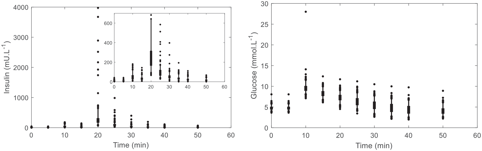Both boluses were numerically considered to occur instantaneously (although they occurred sequentially at the 6 minute time point), and thus were modelled as triangle functions over a period of ∆t $Δ t$ = 12 seconds (forward simulation was undertaken at a resolution of 6 seconds). Blood samples were drawn at t = 0, 5, 10, 15, 20, 25, 30, 35, 40, and 50 minutes. Glucose was measured immediately from each sample (Enzymatic glucose hexokinase assay, Abbot Labs, Illinois, USA), then the remaining sample was spun and frozen for later batch assay of insulin and C-peptide (ELISA Immunoassay, Roche, Germany). Population summaries of the insulin and glucose data from the 212 tests are plotted in Figure 1.

Figure 1.

Population summary of insulin and glucose profiles. The thick error bars show the interquartile range, thin error bars show the 5th to 95th percentile range, and the dots show the outlying points. The child plot contained in the top right of the insulin graph crops the y-axis of the original graph to omit outlier samples.

DISST Model

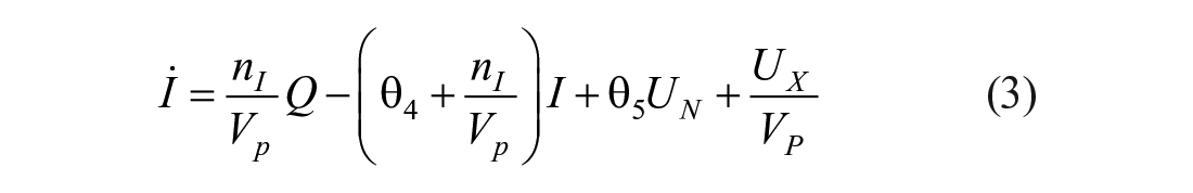
The DISST model defines glucose, insulin and C-peptide kinetics.² C-peptide and insulin concentrations are modelled as two-compartment models, while glucose is modelled as a single compartment. These models are defined:

\dot{C} = k_{2} Y - (k_{1} + k_{3}) C + U_{N}

(1)

\dot{Y} = k_{1} C - k_{2} Y

(2)

U_{N} = U_{B} + U_{1} (t) + U_{2} (t) + U_{3} (t)

(1a)

U_{B} = k_{3} C_{0}

(1b)

U_{1} (t) = {\begin{matrix} θ_{1} / Δ t, & 6 \leq t \leq 6 + Δ t \\ 0, & o t h e r w i s e \end{matrix}

(1c)

U_{2} (t) = {\begin{matrix} θ_{2} (60 - t) / 54, & 6 \leq t \leq 60 \\ 0, & t < 6 \end{matrix}

(1d)

U_{3} (t) = {\begin{matrix} θ_{3} (t - 60) / 54, & 6 \leq t \leq 60 \\ 0, & t < 6 \end{matrix}

(1e)

\dot{I} = \frac{n_{I}}{V_{p}} Q - (θ_{4} + \frac{n_{I}}{V_{p}}) I + θ_{5} U_{N} + \frac{U_{X}}{V_{P}}

(3)

\dot{Q} = \frac{n_{I}}{V_{Q}} I - (n_{C} + \frac{n_{I}}{V_{Q}}) Q

(4)

\dot{G} = p_{G} (G_{0} - G) - θ_{6} (G Q - G_{0} Q_{0}) + θ_{7} P_{X}

(5)

Mixing Model

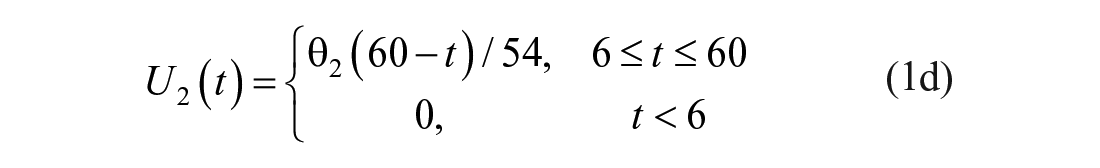
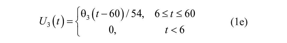
The mixing model introduced in this paper adds additional (local) mixing compartments for the insulin and glucose concentrations to the DISST model, by modifying equations (3) –(5). The additional compartments aim to model non-instantaneous post-bolus mixing. The modifications to the model are:

{\dot{I}}_{1} = - θ_{8} (I_{1} - I_{2}) + θ_{9} U_{X}

(6)

{\dot{I}}_{2} = - θ_{4} I_{2} + \frac{n_{I}}{V_{P}} (Q - I_{2}) + θ_{5} U_{N} - \frac{θ_{9}}{θ_{8} V_{p}} (I_{2} - I_{1})

(7)

\dot{Q} = \frac{n_{I}}{V_{Q}} I_{2} - (n_{C} + \frac{n_{I}}{V_{Q}}) Q

(8)

{\dot{G}}_{1} = - θ_{10} (G_{1} - G_{2}) + θ_{11} P_{X}

(9)

\begin{matrix} {\dot{G}}_{2} = - \frac{θ_{7}}{θ_{11}} θ_{10} (G_{2} - G_{1}) \\ - p_{G} (G_{2} - G_{0}) - θ_{6} (G_{2} Q - G_{0} Q_{0}) \end{matrix}

(10)

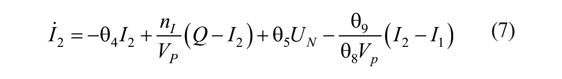
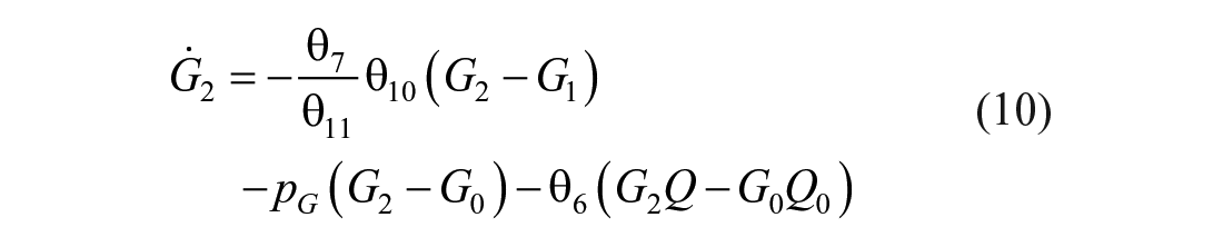
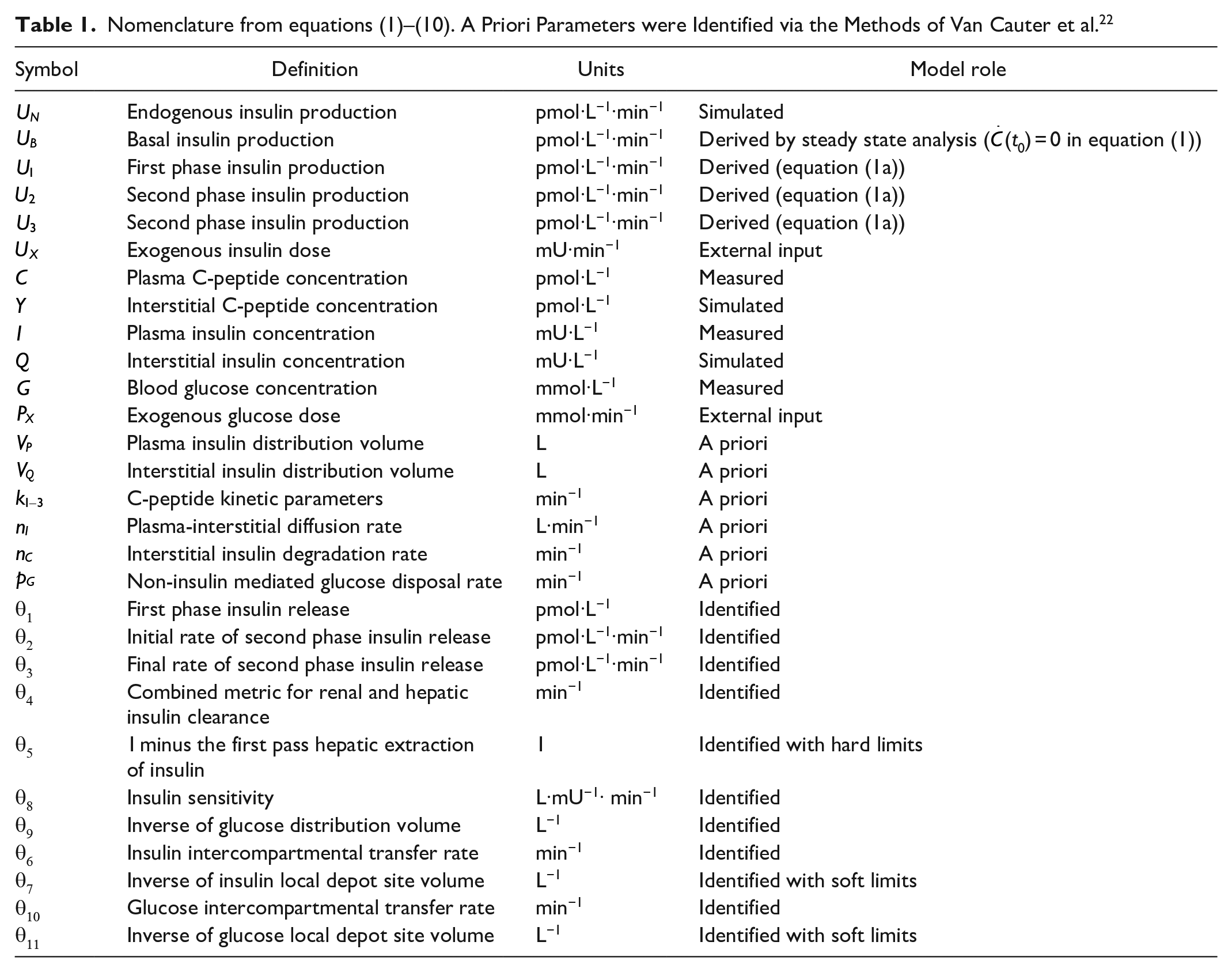
where: equation nomenclature is shown in Table 1.

Table 1.

Nomenclature from equations (1) –(10). A Priori Parameters were Identified via the Methods of Van Cauter et al.²²

Symbol	Definition	Units	Model role
$U_{N}$	Endogenous insulin production	pmol∙L⁻¹∙min⁻¹	Simulated
$U_{B}$	Basal insulin production	pmol∙L⁻¹∙min⁻¹	Derived by steady state analysis ( $\dot{C}$ (t₀) = 0 in equation (1))
$U_{1}$	First phase insulin production	pmol∙L⁻¹∙min⁻¹	Derived (equation (1a))
$U_{2}$	Second phase insulin production	pmol∙L⁻¹∙min⁻¹	Derived (equation (1a))
$U_{3}$	Second phase insulin production	pmol∙L⁻¹∙min⁻¹	Derived (equation (1a))
$U_{X}$	Exogenous insulin dose	mU∙min⁻¹	External input
$C$	Plasma C-peptide concentration	pmol∙L⁻¹	Measured
$Y$	Interstitial C-peptide concentration	pmol∙L⁻¹	Simulated
$I$	Plasma insulin concentration	mU∙L⁻¹	Measured
$Q$	Interstitial insulin concentration	mU∙L⁻¹	Simulated
$G$	Blood glucose concentration	mmol∙L⁻¹	Measured
$P_{X}$	Exogenous glucose dose	mmol∙min⁻¹	External input
$V_{P}$	Plasma insulin distribution volume	L	A priori
$V_{Q}$	Interstitial insulin distribution volume	L	A priori
$k_{1 - 3}$	C-peptide kinetic parameters	min⁻¹	A priori
$n_{I}$	Plasma-interstitial diffusion rate	L∙min⁻¹	A priori
$n_{C}$	Interstitial insulin degradation rate	min⁻¹	A priori
$p_{G}$	Non-insulin mediated glucose disposal rate	min⁻¹	A priori
$θ_{1}$ θ₁	First phase insulin release	pmol∙L⁻¹	Identified
$θ_{2}$	Initial rate of second phase insulin release	pmol∙L⁻¹∙min⁻¹	Identified
$θ_{3}$	Final rate of second phase insulin release	pmol∙L⁻¹∙min⁻¹	Identified
$θ_{4}$	Combined metric for renal and hepatic insulin clearance	min⁻¹	Identified
$θ_{5}$	1 minus the first pass hepatic extraction of insulin	1	Identified with hard limits
$θ_{8}$	Insulin sensitivity	L∙mU⁻¹∙ min⁻¹	Identified
$θ_{9}$	Inverse of glucose distribution volume	L⁻¹	Identified
$θ_{6}$	Insulin intercompartmental transfer rate	min⁻¹	Identified
$θ_{7}$	Inverse of insulin local depot site volume	L⁻¹	Identified with soft limits
$θ_{10}$	Glucose intercompartmental transfer rate	min⁻¹	Identified
$θ_{11}$	Inverse of glucose local depot site volume	L⁻¹	Identified with soft limits

Parameter Identification Methods

This analysis compares and contrasts the identified model values and residuals from 3 implementations of the DISST model identification. The first implementation uses the typical Levenberg-Marquardt identification method (LM) with a downsampled data set (DS). In this downsampled dataset, the insulin data point immediately after the insulin bolus is ignored during identification and the 2 glucose data points that occur immediately after the glucose bolus are also ignored during identification. The DISST model of equations (1)–(5) are used in this analysis.

The second method utilizes a simple LM method with the mixing model additions to the simple DISST model. In particular, equations (1) and (2), (6)–(10) are used for the mixing model analysis (LcM). In initial analysis, the model yielded parameter values indicative of practical non-identifiability.²³ These values are shown in Appendix A. The Differential Algebra for Identifiability of SYstems (DAISY) software tool²⁴ was used to establish that the model of equations (1) and (2), (6)–(10) was structurally identifiable.

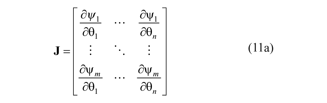
During parameter identification, the $θ_{9}$ and $θ_{11}$ values were constrained towards 10 L⁻¹ (0.1 L) by a penalty term added to the residual to avoid poor capture of model values for the mixing model. The weighting of this influence factor was different across the glucose and insulin model due to the different typical numerical magnitudes of the different species, and was determined empirically for this analysis. In particular, the residual shown in equation (11b) was adapted to equation (11c). This formulation follows the general formulation described by equation (2). Additionally, hepatic clearance rates were limited to a physiologically feasible range of [0.05, 0.95].

Finally, the adapted Levenberg Marquardt method (aLM) is used with the original DISST model of equations (1)–(5). The original Levenberg-Marquardt parameter identification approach iterates towards the optimal parameter set ( $θ_{o p t}$ ) with the iterative process:

θ_{i + 1} = θ_{i} - {(J^{T} J + λ \cdot d i a g (J^{T} J))}^{- 1} J^{T} ψ

(11)

where:

J = [\begin{matrix} \frac{\partial ψ_{1}}{\partial θ_{1}} & \dots & \frac{\partial ψ_{1}}{\partial θ_{n}} \\ ⋮ & ⋱ & ⋮ \\ \frac{\partial ψ_{m}}{\partial θ_{1}} & \dots & \frac{\partial ψ_{m}}{\partial θ_{n}} \end{matrix}]

(11a)

ψ = [X (θ_{i}, t_{j}) - X_{M, j}] = [\begin{matrix} X (θ_{i}, t_{1}) - X_{M, 1} \\ X (θ_{i}, t_{2}) - X_{M, 2} \\ ⋮ \\ X (θ_{i}, t_{m}) - X_{M, m} \end{matrix}]

(11b)

\begin{array}{l} ψ_{i n s u l i n} = [\begin{matrix} X (θ_{i}, t_{j}) - X_{M, j} \\ 250 (θ_{9, i} - 10) \end{matrix}] \\ ψ_{g l u c o s e} = [\begin{matrix} X (θ_{i}, t_{j}) - X_{M, j} \\ 5 (θ_{11, i} - 10) \end{matrix}] \end{array}

(11c)

and $J$ is the Jacobian of residuals with respect to variance in $θ_{i}$ , $ψ$ is the residual vector, $X$ is the measured property; $j$ is the sample index from 1 to m where m is the number of samples ( $j \in (1, 2, \dots m)$ ; $X (θ_{i}, t_{j})$ is the modelled value of $X$ at $t = t_{j}$ ; and $X_{M, j}$ is the measured value of $X$ at $t = t_{j}$ . For this analysis, the damping term $λ$ was chosen with the strategy suggested by Marquardt.⁹

The aLM method was designed to dissipate the contribution of outlying data on the identification of $θ_{o p t}$ .¹² Importance of residuals is modulated with an operator-independent assessment of data-point reliability similar to the long-established class of M-estimators.^25,26 However, adapted method differs to these estimators through its use of the Jacobian in (11a). Ultimately, the aLM substitutes $\hat{ψ}$ for $ψ$ , yielding:

θ_{i + 1} = θ_{i} - (J^{T} J + λ \cdot d i a g (J^{T} J))^{- 1} J^{T} \hat{ψ}

(12)

where:

\overset{\land}{ψ} = ψ ⊙ \exp (\frac{- | ψ |}{β {| ψ |}_{M}})

(12a)

and ${| ψ |}_{M}$ is the median of the absolute values of the residuals and $β$ is a scaling factor that determines the aggression of the outlier down-weighting as a function of ${| ψ |}_{M}$ . A $β$ of 3 was used as this is in accordance with accepted statistical basis for rejection of outlier data (ie, 3 standard deviations).^27,28

All implementations of the model were identified in segments.

Parameters $θ_{1 - 3}$ of the C-peptide model (equations (1) and (2)) were identified using only C-peptide data.

Parameters $θ_{4 - 5}$ (and $θ_{8 - 9}$ for LcM) of the insulin models (equations (3) and (4) for DS and aLM; equations (6)–(8) for LcM) were identified using insulin data and the $U_{N}$ profile from the C-peptide identification.

Parameters $θ_{6 - 7}$ (and $θ_{10 - 11}$ for LcM) the glucose models (equation (5) for DS and aLM; equations (9) and (10) for LcM) were identified using glucose data and the $Q$ profile from insulin identification.

Analyses and Performance Evaluation

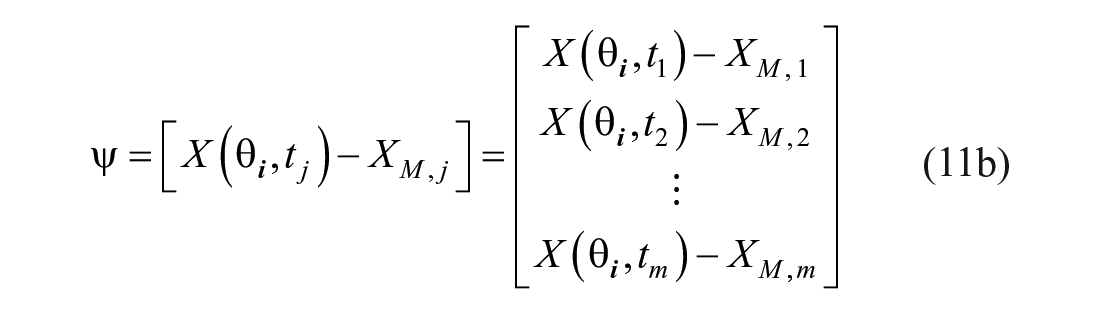
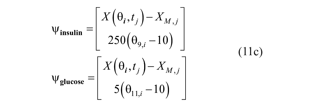
The 3 implementations are qualitatively compared using model residuals. Since each model optimises a different residual $(ψ, ψ = ψ_{2})$ , the methods cannot be directly, quantitatively compared. To highlight differences in implementation outcomes, both summary statistics of $ψ$ values and residuals as a function of time ( $ψ$ ) are presented. Parameters obtained from each implementation will be compared for agreement. Identified parameter values are compared using Spearman’s rank correlations for each implementation, as a few cases with extreme parameter values invalidate the linearity assumption of the more common Pearson correlation.²⁹

For each model implementation, a Monte Carlo analysis³⁰ was performed on all trials as follows:

Measurements were simulated from the given trial’s identified parameter values.

Normally distributed relative error ( $σ = 4 %$ ) was added to the simulated measurements to generate 100 sets of noisy data.

Model parameters were identified for each noisy dataset, yielding 100 parameter estimates.

The coefficient of variation (CV) for each parameter was calculated.

Summary statistics of the CV values from all 212 trials are presented. These values are indicative of practical parameter identifiability and stability for the given implementation.

Results

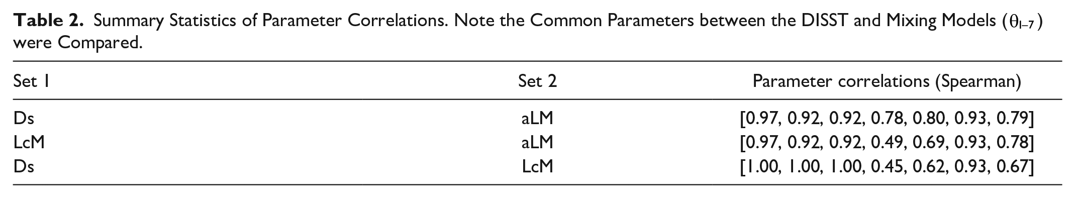
Correlations between the identified parameter values across the different model implementations are presented in Table 2. The aLM parameters and DS parameters correlated well. The LcM parameters did not correlate well with either the aLM or DS parameters, with the exception of the insulin sensitivity parameter $θ_{6} .$ Comparisons of $θ_{6}$ values obtained through the 3 implementations are presented in Figure 2. Two model responses, of moderate and extreme outliers are shown in Figures 3 and 4, respectively.

Table 2.

Summary Statistics of Parameter Correlations. Note the Common Parameters between the DISST and Mixing Models ( $θ_{1 - 7}$ ) were Compared.

Set 1	Set 2	Parameter correlations (Spearman)
Ds	aLM	[0.97, 0.92, 0.92, 0.78, 0.80, 0.93, 0.79]
LcM	aLM	[0.97, 0.92, 0.92, 0.49, 0.69, 0.93, 0.78]
Ds	LcM	[1.00, 1.00, 1.00, 0.45, 0.62, 0.93, 0.67]

Figure 2.

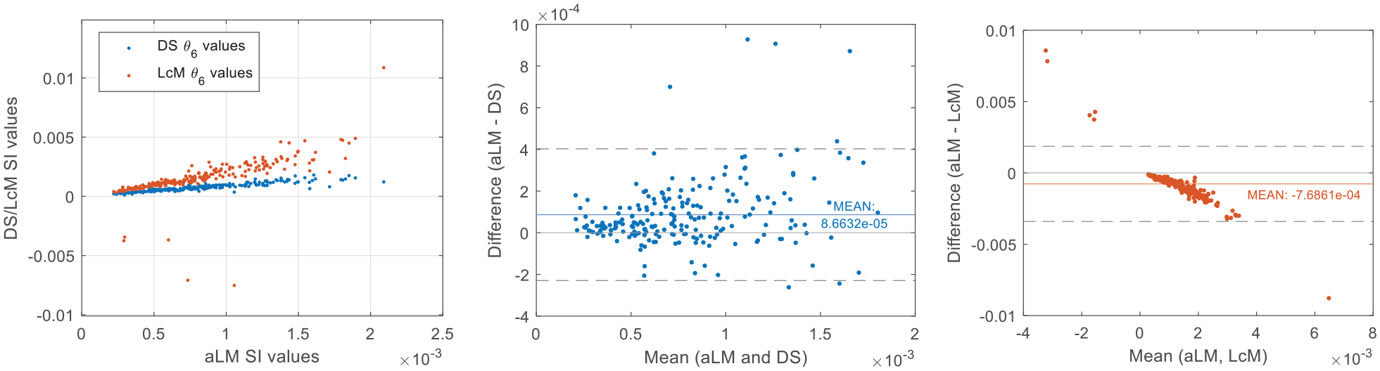
Comparison of insulin sensitivity (SI) values identified by each implementation and Bland Altman plots showing agreement across implementations.

Figure 3.

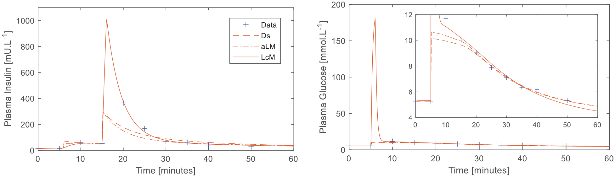
Plasma insulin and glucose responses to the DISST test with moderate outliers to the simple model in the insulin (t = 20, and 25 minutes) and glucose data (t = 10 minutes). Child plot displays parent plot with cropped y-axis for clarity.

Figure 4.

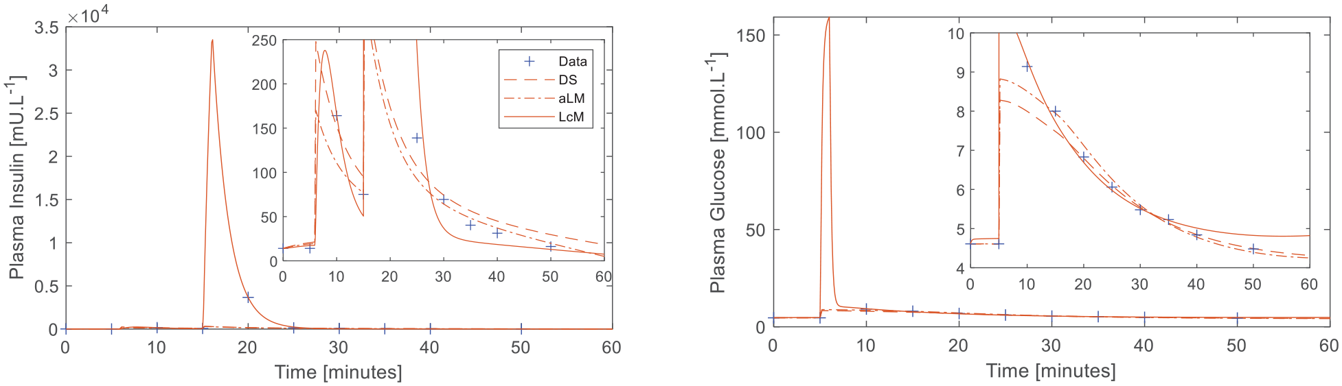
Plasma insulin and glucose responses to the DISST test with significant outliers in the insulin data and moderate outliers in the glucose data. The inset plots display parent plots with cropped y-axes for clarity.

Summary statistics of absolute residuals $ψ$ of each implementation are presented in Table 3 and they include residuals from data points which were ignored, or had reduced influence during identification. The DS and aLM implementations show a greater range of errors between high and low percentiles. This spread indicates that ignoring outliers improved smaller residuals at the cost of increased large residuals.

Table 3.

Summary Statistics of Absolute Errors across All Trials. Note that the Errors in DS and aLM Include Errors for Full Dataset to Enable Direct Comparison.

Model	Implementation	Percentiles of absolute residuals
Model	Implementation	[ψ25, ψ50, ψ75, ψ95, ψ99]
C-peptide [pmol.L⁻¹]	Ds/LcM	[7.58, 22.6, 47.6, 103, 197]
C-peptide [pmol.L⁻¹]	aLM	[1.16, 12.6, 45.9, 134, 295]
Insulin [mU.L⁻¹]	Ds	[2.32, 5.51, 14.2, 109, 334]
	aLM	[1.44, 4.01, 11.4, 112, 345]
	LcM	[1.87, 4.79, 9.86, 31.1, 93.8]
Glucose [mmol.L⁻¹]	Ds	[0.04, 0.12, 0.28, 1.15, 2.09]
	aLM	[0.02, 0.08, 0.24, 0.89, 1.70]
	LcM	[0.04, 0.12, 0.25, 0.57, 1.02]

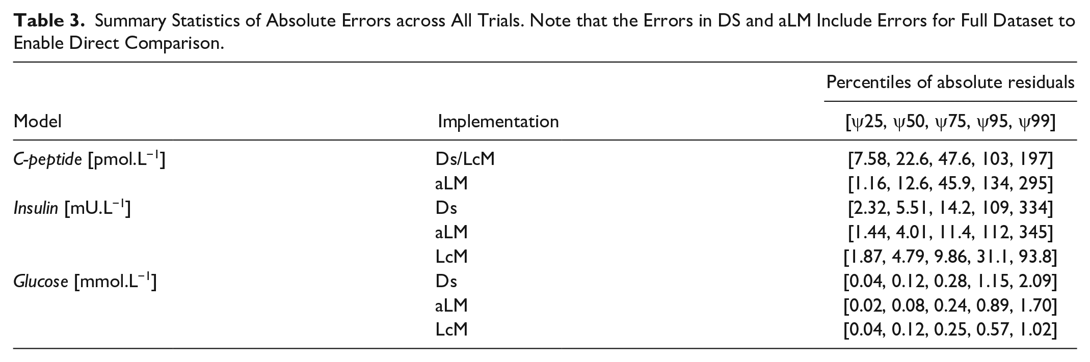
Figure 5 shows the distribution of the residuals. C-peptide samples are relatively well-centered about zero and follow a seemingly normal distribution across the samples. In contrast, both insulin and glucose residuals were sporadic showing biases during the mixing phases at t = 20 minutes for insulin, and t = 10 minutes for glucose. The LcM is well centered around the immediate post-bolus point for insulin, but exhibits bias at the surrounding samples. The glucose data are well centered with the LcM except for a small bias on the final sample.

Figure 5.

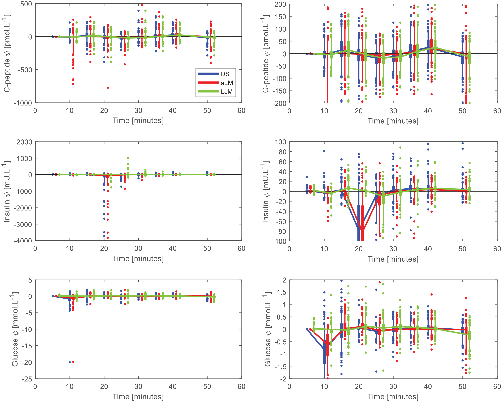
Residual plots for C-peptide, insulin, and glucose. The plots on the right are cropped to show the general behavior. The thick error rs show the interquartile range, thin error bars show the 5th to 95th percentile range, and the dots show the outlying points. The time points are offset for aLM and DS to enable clearer observation.

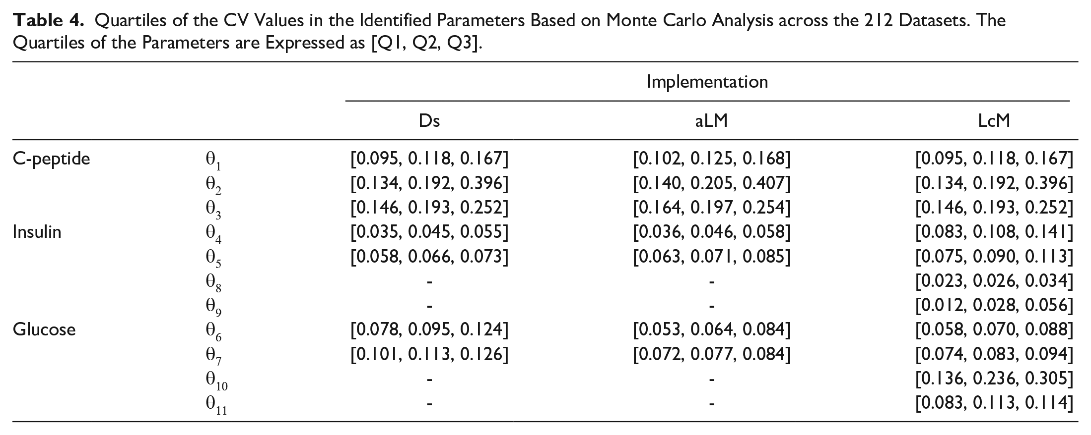
Finally, Table 4 summarizes the Monte Carlo analysis of the 3 implementations. The additional parameters introduced by the mixing model had relatively low CV values in the insulin model of equations (6)–(8), but high values for the glucose model of equations (9) and (10). For parameters comparable to the DISST model, the mixing model had increased CV values for insulin, relative to the DS and aLM implementations. The comparable glucose parameters identified by the mixing model had CV values slightly greater than aLM, but lower than DS.

Table 4.

Quartiles of the CV Values in the Identified Parameters Based on Monte Carlo Analysis across the 212 Datasets. The Quartiles of the Parameters are Expressed as [Q1, Q2, Q3].

		Implementation
		Ds	aLM	LcM
C-peptide	$θ_{1}$ θ₁	[0.095, 0.118, 0.167]	[0.102, 0.125, 0.168]	[0.095, 0.118, 0.167]
	$θ_{2}$	[0.134, 0.192, 0.396]	[0.140, 0.205, 0.407]	[0.134, 0.192, 0.396]
	$θ_{3}$	[0.146, 0.193, 0.252]	[0.164, 0.197, 0.254]	[0.146, 0.193, 0.252]
Insulin	$θ_{4}$	[0.035, 0.045, 0.055]	[0.036, 0.046, 0.058]	[0.083, 0.108, 0.141]
	$θ_{5}$	[0.058, 0.066, 0.073]	[0.063, 0.071, 0.085]	[0.075, 0.090, 0.113]
	$θ_{8}$	-	-	[0.023, 0.026, 0.034]
	$θ_{9}$	-	-	[0.012, 0.028, 0.056]
Glucose	$θ_{6}$	[0.078, 0.095, 0.124]	[0.053, 0.064, 0.084]	[0.058, 0.070, 0.088]
	$θ_{7}$	[0.101, 0.113, 0.126]	[0.072, 0.077, 0.084]	[0.074, 0.083, 0.094]
	$θ_{10}$	-	-	[0.136, 0.236, 0.305]
	$θ_{11}$	-	-	[0.083, 0.113, 0.114]

Discussion

Figure 5 shows the LcM was able to capture the mixing behavior in glucose and insulin data. In particular, the residuals of the LcM for both insulin and glucose surrounding the bolus are smaller and less biased than those of DS and aLM. Both DS and aLM typically missed the post-bolus data points. However, this was the intended outcome of the DS implementation, and the aLM was specifically designed to miss such aberrant points.

In terms of model simulation, Figure 5 also shows the DS and aLM implementations performed in roughly the same way. This indicates the manual removal of isolated data points that are affected by unmodelled mixing yields proximal results to the aLM implementation. Since the aLM implementation is based on the statistically justified implementation of declaring data 3 standard deviations from the mean as outliers, the DS implementation may assume a similar justification by proxy of the parameter and residual outcomes.

Despite the relative homogeny of the test cohort, the DS and aLM implementations achieved high correlations (ρ ~0.9) between most parameters (Table 2). Of note, the LcM had lower correlations for most parameters except the insulin sensitivity term ( $θ_{6}$ ). This latter result is important as insulin sensitivity is an important metabolic marker for many applications.^31-33 While large differences in parameters values across DS or aLM and LcM were expected due to the increased complexity and changed internal dynamics of the LcM, the high Spearman correlation of 0.93 for $θ_{6}$ was unexpected. However, this correlation may be explained by the inability of the adaptations made to the LcM to capture the glucose data indicative of insulin-mediated glucose disposal.

In particular, all implementations must conform to the data between t = 20 to 50 minutes with much the same modelled dynamics. The trend visible in Figure 2 indicates with an empirical scaling equation, such as a linear fit, the mixing model could identify the primary metric of interest in glycemic modelling^1,31,34,35 despite its difference in insulin identification.

In the typical case shown in Figure 3, the LcM was able to capture the data affected by mixing dynamics as well as the other stages of the test. However, for the case shown in Figure 4, the large insulin outlier at approximately t = 20 minutes had a disproportionate effect on the model, and thus the simulation failed to fit the data appropriately after the mixing phase. The LcM residual plots in Figure 5 show the mixing model exhibits low error in the immediate post bolus data, but higher error for samples outside of mixing data time periods. This outcome indicates more cases fit the behavior shown in Figure 4, which is a less desirable result.

The residuals described in Table 3 also demonstrate the general agreement between DS and aLM, although there are some minor differences. For insulin, aLM exhibited a larger range between residual percentiles then DS, indicating further outlier down-weighting occurred for samples other than the t = 20 minute sample. Glucose residuals for aLM were lower than DS across all percentiles, which indicates un-modelled mixing behaviour in glucose is not always outlying for both the t = 10 and t = 15 minute samples. The mixing model’s ability to capture mixing behavior was demonstrated through the relatively low LcM residuals in the higher percentiles.

Table 4 shows the DS and aLM identified insulin model parameters with approximately half the variance as the LcM. This difference quantifies the risk of increased parameter trade off with increased parameterization.³⁶ In contrast, the glucose model parameters show an almost reversed trend, where the LcM had similar CV values for insulin sensitivity and volume ( $θ_{6}$ and $θ_{7}$ ), but relatively high (CV) values for the glucose mixing parameters.

The contrast between these results can be explained with the difference in the nature of the outliers in insulin and glucose. The mixing points in insulin are much greater relative to the surrounding points, exhibiting strong mixing behavior captured by the mixing terms in the LcM. However, the mixing dynamics added can overtly influence the identification and miss the insulin dynamics contained in later samples. This trade off led to poor parameter stability for $θ_{4 - 5}$ . The mixing in glucose data was generally faster and smaller, and this smaller influence led to potential elimination of the effects of unmodelled post bolus dynamics on the identification of insulin sensitivity.

The comparable stability of $θ_{6 - 7}$ identification contradicts assumptions of the Akaike information criterion and could be explained by the mixing model’s tendency to favor the glucose fit of the t = 50 minutes sample less than the other samples (shown in Figure 5). This behavior leads to a prioritization of points containing more information on the glucose kinetics. However, the stability of identified insulin sensitivity values in the LcM model was concomitant with reduced identification accuracy for glucose mixing parameters.

This study modified the adapted GN algorithm of Gray et al.¹² to include the more sophisticated Levenberg-Marquardt algorithm. While the DS and aLM methods were stable with the GN and adapted GN algorithms, respectively, the more complex LcM was susceptible to instability due to its higher dimensionality and more extreme behavior in capturing mixing. Hence, the Levenberg Marquardt algorithm was used as a basis for all implementations to allow more consistent and comparable results.

In addition, further adjustments were required to ensure the mixing model obtained results in a feasible parameter region. These adjustments necessitated the use of a penalty function to restrict the mixing volume parameters and a boundary to prevent $θ_{4}$ from reaching physically infeasible values. The spread of LcM parameters when unconstrained is shown in Appendix A and justifies the decision to constrain or limit LcM parameters to feasible values. Equally, the spread of parameters in the unconstrained LcM is indicative of a practically non-identifiable model.³⁷ However, it must be noted that there are many possible implementations of mixing models, and such numerical identifiability issues must be assessed directly within each candidate. For example, a two-compartment labelled Minimal Model¹⁸ is able to identify parameters in addition to those identified by the foundational iteration of the model.¹ In contrast to the DISST, the sampling protocol required for the labelled Minimal Model is model has a higher number and frequency of samples and uses a traceable glucose bolus. The labelled Minimal Model is able to determine a profile for endogenous glucose production, and values of glucose effectiveness, insulin sensitivity, and plasma clearance rate. Similar to the DISST, a two-compartment unlabelled Minimal Model, was found to have comparable identifiability issues to the LcM unless a priori knowledge was incorporated.

The foundational DISST model assumes first order hepatic clearance of glucose^2,38 and also defines the more complex insulin/glucose dynamic as a secondary glucose clearance pathway. Other models contain further complexity. However, the complexity of these models are not well suited to the low sampling frequency of the DISST protocol.^23,39

It should also be noted this LcM implementation was phenomenological, rather than explicitly mechanistic. Complex physiological mixing mechanisms were simplified into a local mixing compartment with a diffusion-driven mixing rate. With the limited data available from the DISST tests, this phenomenological explanation for mixing behavior can mitigate the risk of over-parameterization and also yields a stable insulin sensitivity ( $θ_{6}$ ) metric. However, while the model can accurately capture the mixing behavior, it is limited in its inability to predict dynamics in alternative testing protocols.

There is some difficulty comparing LcM results with those of the simple DISST model implementations. While agreement between the down-sampled and adapted methods indicates consistency with the estimation of insulin sensitivity, the values obtained may not accurately reflect those obtained through an alternate testing protocol, such as the hyper-physiological, gold-standard hyperinsulinemic-euglycemic clamp. However, the agreement between the DISST model and mixing model in insulin sensitivity estimation shows sufficient agreement of methods to determine the relevance of modelling mixing behavior, despite the lack of a reference model.

Overall, modelling data exhibiting mixing behavior in the DISST model and method does not provide significant benefits. While there is a potential for improved robustness in identification of insulin sensitivity, there are drawbacks in model implementation due to increased model complexity. This analysis was also undertaken on the 50 minute DISST, which is more intensive than the more recent and equally accurate 30 minute DISST protocol.^40,41 The 30 minute DISST would not have sufficient post-bolus data to enable identification of mixing parameters without significant reliance on a-priori information.

Furthermore, the LcM presented in this research requires further direct comparison and adjustment with respect to a well-established metric, such as the hyperinsulinemic-euglycemic clamp technique, for results to be considered reliable for clinical use. Unless such a study is conducted, the foundation DISST model presented in equations (1)–(5) remains a strong candidate for use due to its relative ease of implementation and robustness, provided an appropriate method is used to handle outlier data influenced by mixing.

Conclusions

This analysis compares the performance of a mixing model with a simpler model, where outliers were either manually removed or detected with an adapted LM method. These methods were tested on noisy data containing varying levels of mixing behavior. The mixing model effectively captured mixing behavior and showed consistency in identifying insulin sensitivity at the cost of increased calibration and complexity in the parameter identification process. While a mixing model could potentially identify some glucose metabolism parameters more accurately while also capturing mixing behavior, the foundation DISST model with an outlier handling process achieves greater consistency at a lower operational cost, and sufficiently captures behavior outside of the outlier points.

Overall, this analysis showed data affected by mixing in intravenous metabolic tests, or similar clinical tests, can be modelled through a mixing compartment model. However, this more complex implementation currently offers minimal benefit over a simpler model with outlier detection. This paper demonstrates the merit of adding mixing compartments to the existing DISST model is primarily in capturing the dynamics of mixing behavior, rather than significantly improving the identification of clinically important parameters. In the context of the DISST, this justifies removal of data in the immediate period after the boluses, though it is worth noting that other models based on tests with less sparse sampling protocols could benefit from the implementation of a local mixing compartment.

Footnotes

Appendix A

Figures A1 and A2 show the parameters identified across the 212 trials with and without constraints on the L-M method. Parameters are ranked from lowest to highest to give a general indication of parameter spread. One trial failed to converge in the unconstrained process due to numerical instability.

Acknowledgements

None

Abbreviations

aLM, adapted Levenberg Marquardt; CV, Coefficient of variation; DAISY, Differential Algebra for Identifiability of SYstems; DISST, Dynamic Insulin Sensitivity and Secretion Test; DS, downsampled; IVGTT, intravenous glucose tolerance test; LcM, Local mixing; LM, Levenberg-Marquardt.

Declaration of Conflicting Interests

The author(s) declared no potential conflicts of interest with respect to the research, authorship, and/or publication of this article.

Funding

The author(s) received no financial support for the research, authorship, and/or publication of this article.

ORCID iDs

Rua Murray

Paul Docherty

References

Bergman

Ider

Bowden

Cobelli

Quantitative estimation of insulin sensitivity. Am J Physiol. 1979;236:E667-E677.

Lotz

Chase

McAuley

, et al Design and clinical pilot testing of the model-based dynamic insulin sensitivity and secretion test (DISST). J Diabetes Sci Technol. 2010;4(6):1408-1423.

Garcia-Estevez

Araujo-Vilar

Fiestras-Janeiro

Saavedra-Gonzalez

Cabezas-Cerrato

Comparison of several insulin sensitivity indices derived from basal plasma insulin and glucose levels with minimal model indices. Horm Metab Res. 2003;35(1):13-17.

Monzillo

Hamdy

Evaluation of insulin sensitivity in clinical practice and in research settings. Nutr Rev. 2003;61(12):397-412.

Bard

Comparison of gradient methods for the solution of nonlinear parameter estimation problems. SIAM J Numer Anal. 1970;7(1):157-186.

Davidon

Variable metric method for minimization. SIAM J Optim. 1991;1(1):1-17.

Docherty

Chase

David

Characterisation of the iterative integral parameter identification method. Med Biol Eng Comput. 2012;50(2):127-134.

Levenberg

A method for the solution of certain non-linear problems in least squares. Q Appl Math. 1944;2:164-168.

Marquardt

DW.

An algorithm for least-squares estimation of nonlinear parameters. SIAM J Appl Math. 1963;11(2):431-441.

10.

Steihaug

The conjugate gradient method and trust regions in large scale optimization. SIAM J Numer Anal. 1983;20(3):626-637.

11.

Sheiner

Beal

SL.

Pharmacokinetic parameter estimates from several least squares procedures: superiority of extended least squares. J Pharmacokinet Biopharm. 1985;13(2):185-201.

12.

Gray

RAL

Docherty

Fisk

Murray

. A modified approach to objective surface generation within the Gauss-Newton parameter identification to ignore outlier data points. Biomed Signal Process Control. 2016;30:162-169.

13.

Smith

Coit

. Constraint handling techniques—penalty functions. In: Bäck

Fogel

Michalewicz

, eds. Handbook of Evolutionary Computation. Vol. 97, No. 1. Oxford University Press and Institute of Physics Publishing; 1997:C5.

14.

Golub

Hansen

O’Leary

DP.

Tikhonov regularization and total least squares. SIAM J Matrix Anal Appl. 1999;21(1):185-194.

15.

Edsberg

Herly

Hildebrandt

Kuhl

Insulin bolus given by a sprinkler needle: effect on absorption and glycaemic response to a meal. Br Med J. 1987;294(6584):1373-1376.

16.

Docherty

Gray

RAL

Mansell

Reducing the effect of outlying data on the identification of insulinaemic pharmacokinetic parameters with an adapted Gauss-Newton approach. In: Boje

, ed. IFAC 19th World Congress. Cape Town, South Africa; 2014.

17.

Lam

Docherty

Chase

Murray

Te Morenga

Using the adapted Levenberg-Marquardt method to determine the validity of ignoring insulin and glucose data that is affected by mixing. In: by Findeisen

Hirche

Janschek

Mönnigmann

, eds. 21st IFAC World Congress. Berlin, Germany, 2020.

18.

Caumo

Vicini

Zachwieja

, et al Undermodeling affects minimal model indexes: insights from a two-compartment model. Am J Physiol. 1999;276:E1171-E1193.

19.

Regittnig

Trajanoski

Leis

, et al Plasma and interstitial glucose dynamics after intravenous glucose injection: evaluation of the single-compartment glucose distribution assumption in the minimal models. Diabetes. 1999;48(5):1070-1081.

20.

Te Morenga

Williams

Brown

Mann

JI.

Effect of a relatively high protein, high fiber diet on body composition and metabolic risk factors in overweight women. Eur J Clin Nutr. 2010;64(11):1323-1331.

21.

Te Morenga

Docherty

Williams

Mann

JI.

The effect of a diet moderately high in protein and fiber on insulin sensitivity measured using the dynamic insulin sensitivity and secretion test. Nutrients. 2017;9(12):1291.

22.

Van Cauter

Mestrez

Sturis

Polonsky

. Estimation of insulin secretion rates from C- peptide levels. Comparison of individual and standard kinetic parameters for C-peptide clearance. Diabetes. 1992;41:368-377.

23.

Docherty

Chase

Lotz

Desaive

A graphical method for practical and informative identifiability analyses of physiological models: a case study of insulin kinetics and sensitivity. Biomed Eng Online. 2011;10(39).

24.

Bellu

Saccomani

Audoly

D’Angio

DAISY: a new software tool to test global identifiability of biological and physiological systems. Comput Methods Programs Biomed. 2007;88(1):52-61.

25.

Farcomeni

Ventura

An overview of robust methods in medical research. Stat Methods Med Res. 2012;21(2):111-133.

26.

Banaś

Ligas

Empirical tests of performance of some M – estimators. Geodesy Cartogr. 2014;63(2):127-146.

27.

Pukelsheim

The three sigma rule. Am Stat. 1994;48(2):88-91.

28.

Bakar

Mohemad

Ahmad

Deris

. A Comparative Study for Outlier Detection Techniques in Data Mining. In: 2006 IEEE Conference on Cybernetics and Intelligent Systems, 2006:1-6.

29.

Hauke

Kossowski

Comparison of values of Pearson’s and Spearman’s correlation coefficients on the same sets of data. Quaest Geogr. 2011;30(2):87-93.

30.

Miao

Xia

Perelson

On identifiability of nonlinear ODE models and applications in viral dynamics. SIAM Rev. 2011;53(1):3-39.

31.

Ferrannini

Natali

Bell

Cavallo-Perin

Lalic

Mingrone

Insulin resistance and hypersecretion in obesity. European Group for the Study of Insulin Resistance (EGIR). J Clin Invest. 1997;100(5):1166-1173.

32.

Martin

Warram

Krolewski

Bergman

Soeldner

Kahn

CR.

Role of glucose and insulin resistance in development of type 2 diabetes mellitus: results of a 25-year follow-up study. Lancet. 1992;340(8825):925-929.

33.

Vozarova

Weyer

Lindsay

Pratley

Bogardus

Tataranni

PA.

High white blood cell count is associated with a worsening of insulin sensitivity and predicts the development of type 2 diabetes. Diabetes. 2002;51(2):455-461.

34.

Haffner

D’Agostino

Jr Mykkanen

, et al Insulin sensitivity in subjects with type 2 diabetes. Relationship to cardiovascular risk factors: the Insulin Resistance Atherosclerosis Study. Diabetes Care. 1999;22(4):562-568.

35.

Hovorka

Shojaee-Moradie

Carroll

, et al Partitioning glucose distribution/transport, disposal, and endogenous production during IVGTT. Am J Physiol Endocrinol Metab. 2002;282(5):E992-1007.

36.

Mansell

Schmidt

Docherty

Nørgaard

Jørgensen

Madsen

Evaluation of model designs for subcutaneous infusion of insulin aspart. J Pharmacokinet Pharmacodyn. 2017;44(5):477-489.

37.

Raue

Kreutz

Maiwald

Bachmann

Schilling

Klingmüller

Structural and practical identifiability analysis of partially observed dynamical models by exploiting the profile likelihood. Bioinformatics. 2009;25.

38.

Thorsteinsson

Kinetic models for insulin disappearance from plasma in man. Dan Med Bull. 1990;37(2):143-153.

39.

Cobelli

DiStefano

JJ.

Parameter and structural identifiability concepts and ambiguities: a critical review and analysis. Am J Physiol 1980;239(1):R7.

40.

McAuley

Berkeley

Docherty

, et al The dynamic insulin sensitivity and secretion test—a novel measure of insulin sensitivity. Metabolism. 2011;60(12):1748-1756.

41.

Docherty

Chase

Lotz

, et al A spectrum of dynamic inuslin sensitivity test protocols. J Diabetes Sci Technol. 2011;5(6):1499-1508.

The Effects of Additional Local-Mixing Compartments in the DISST Model-Based Assessment of Insulin Sensitivity

Abstract

Background:

Methods:

Results:

Conclusions:

Keywords

Introduction

Methods

Clinical Protocol

DISST Model

Mixing Model

Parameter Identification Methods

Analyses and Performance Evaluation

Results

Discussion

Conclusions

Footnotes

Appendix A

Acknowledgements

Abbreviations

Declaration of Conflicting Interests

Funding

ORCID iDs

References