Sage Journals: Discover world-class research

Abstract

The design of racing drones brings quite a thrilling challenge from a flight dynamics point of view. This work aims to offer a single-based simulation platform combining its geometric design, trajectory control, and guidance of racing drones. Also, it is reckoned from a pilot’s view in a classic FPV competition. Hence, it is an active platform for studying racing drones’ design founded on dynamics, with fifteen different drone models. It is one of the few existing platforms that combine all aspects of racing drones in a single simulation environment. Also, it is open access via Matlab Central - File Exchange.

Keywords

Racing Airframe racing Drone racing Trajectory high performance structure design air vehicle simulation

Introduction

Computer tools aim to create virtual environments that recreates real complex scenarios. Thus, they usually hold become useful simulation platforms.^1,2 Their benefits have been tested in multiple designs. In addition, they need adjustments to suit the response in different scenarios.^3,4 ⁵

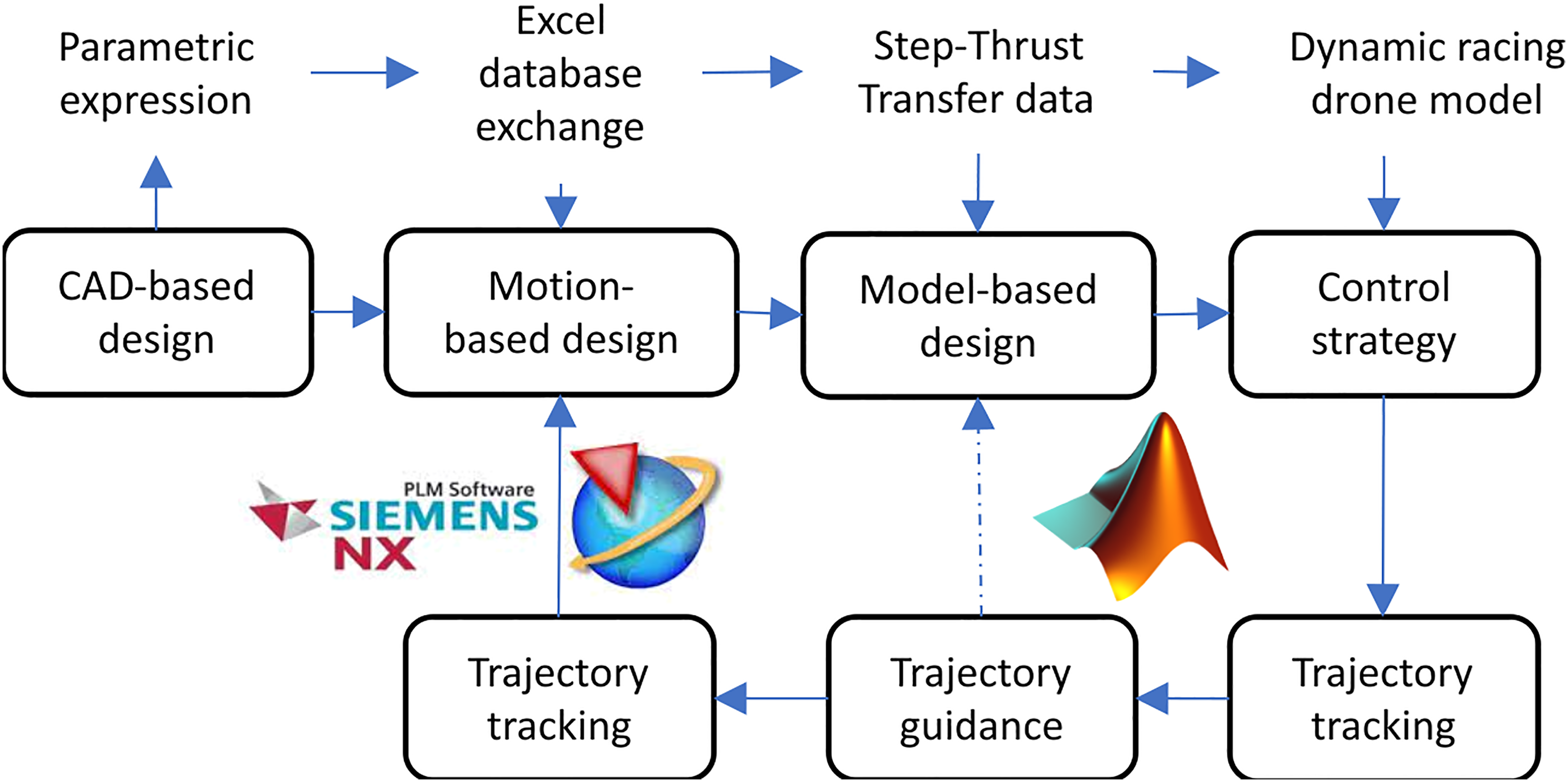
The design of control systems takes the lead of these platforms.⁶ They estimate the drone’s behaviour.^7–10 So, the effects are planned to be helpful in actual active states.^11,12 Indeed, the integration of simulation platforms is not new.^13–16 It seems to have a decisive edge over cost and design times.^17–19 When it comes to evaluating the performance of drones, trading data and tying it jointly on a unique platform would make the design process more precise. The CAx(CAD, CAM, CIM, CFD) tools quickly merged the design cycles.^20–23 However, linking the data with model-based design software needs further support to enrich design methods.^24–27 The work aims to offer a single-based simulation platform. It is for geometric design, trajectory control and guidance of racing drones. Mainly, it combines data from motion-based and model-based design software (see Figure 1). The airframes of the racing drones were drawn in Unigraphics NX^TM software from Siemens Product Lifecycle. Thus, the CAD module holds the mass distributions of the bodies. The motion module is liable for the dynamics of the motors and propellers. In this way, the thrust force is run from it. Simulink^® manages the control design. Here the rigid body dynamics are figured. In addition, the guidance of the racing drone is into it. MATLAB^® is sensitive to running variables. Also, for getting data from NX. Both software packets are from the MathWorks^® Corporation. The right mix of data links will result in racing guidances through waypoints. It means without follow-up policies between points. The trajectories gauged are from a pilot’s view, not an intelligent system. The option to switch between kinds of racing drones is open. Also, the impact on those trajectories can be studied. In this way, it is the only one that combines all aspects of a racing drone in a single simulation environment.

Figure 1.

Co-Simulation platform.

The first section of this paper deals with the equations of motion. It describes the flight dynamics of a racing drone. The second section defines how the thrust force was figured. The mass distribution and the measure of the body torque are also added. The third section handles the technical requirements. It is based on performance metrics by locating the system’s poles. Thus, the controllers’ operating ranges are defined. In addition, the trajectory guidance problem is solved. The last section shows the data flow between the platforms. It is defined how to set up the simulation platform to run multiple experiments with distinct airframe models. In addition, a case study was conducted on the flight dynamics linked to the airframe models to see the platform’s ability.

Equations of motion for a racing drone

The equations of motion explaining flight dynamics are widely issued in the literature.^28–35 They are not for a racing drone. The main simplifications that manage the distinct control methods are laid out.^36–39 It helps to track flight trajectories. Some papers have handled the premises for figuring out the physical effects in mixed ways.^40–45 It is via testing to get coefficients. It can also be through mathematical terms.

\begin{matrix} p = (x, y, z) \\ \frac{d p}{d t} = (\dot{x}, \dot{y}, \dot{z}) \\ \frac{d}{d t} (\frac{d p}{d t}) = \frac{1}{m} (T_{n x} R_{z y x}) - g \end{matrix}

(1)

\begin{matrix} ω = (ϕ, θ, ψ) \\ \frac{d ω}{d t} = R_{z y x} (ω^{T}) \\ \frac{d}{d t} (\frac{d ω}{d t}) = (- ω^{T}) \times I_{n x} ω + τ_{b o d y} \end{matrix}

(2)

Table 1 shows the nomenclature of the variables included. As shown above, the equations are precise way. It describes the motion of a racing drone in detail. It also facilitates the simulations’ numerical math. Suppose the thrust force

(T_{n x})

and the moment of inertia

(I_{n x})

are fetched from the CAD module of NX. In that case, the translational (1) and rotational (2) motion define the dynamics of a racing drone. Where (

m

) is the body’s mass and (

g

) is the acceleration due to gravity force.

Table 1.

Nomenclature of the equations of motion.

Symbol -Variable	Definition - Description
p	Position
$(x, y, z)$	Components of p
$ω$	Angular position
$(ϕ, θ, ψ)$	Components of $ω$
$\frac{d p}{d t}$	Velocity of p
$\frac{d ω}{d t}$	Angular velocity of $ω$
$\frac{d}{d t} (\frac{d p}{d t})$	Acceleration of p
$\frac{d}{d t} (\frac{d ω}{d t})$	Angular acceleration of $ω$
$T_{n x}$	Thrust force - Unigraphics NX
$I_{n x}$	Moment of inertia - Unigraphics NX
$m$	Body’s mass
$g$	Acceleration due to gravity force
$R_{z y x}$	Rotation matrix
$ω^{T}$	antisymmetric matrix of the $ω$
$τ_{b o d y}$	Body torque
$I_{s}$	Tracking of the input signal

Table 2.

Nomenclature of Motor model.

Symbol - Variable	Definition - Description
$I_{s}$	Tracking of the input signal
$L$	Inductance
$K_{e}$	Back EMF constant
$Ω$	Rotor rotational velocity
$R$	Electrical resistance
$i_{a}$	Initial Current
PMDC Motor	Brushless type.
$N_{i n}$	Input dignal to the motor
$ρ$	Air density
$A$	Propeller radius
$v_{u}$	Induced speed
$v_{θ}$	Forward speed

The centre of mass is located in the reference body frame $b o d y f (x, y, z)$ . It is defined by the three components of the angular position ( $ω$ ). The three rectangular components of the point $(p)$ are also defined. It is assumed that this point is placed at the origin of $b o d y f (x, y, z)$ . Then, the translational motion of a racing drone has to be caused. It is caused when the points $(p)$ are accelerated by the angular pitch position rotation sequences ( $θ$ ).

- ω^{T} = [\begin{matrix} 0 & - \dot{ϕ} & \dot{ψ} \\ \dot{ϕ} & 0 & - \dot{θ} \\ - \dot{ψ} & - \dot{θ} & 0 \end{matrix}]

Thus, the rotational motion is achieved when running the cross product between the rotation matrix

R_{z y x}

and the antisymmetric matrix (

- ω^{T}

) of the angular velocities. It takes a steady, stable flight.

The body torque $(τ_{b o d y})$ is usually a formulation linked with the differences between the speeds of the rotors.^46,47,27 In addition, they are mapped as input $(I_{s})$ to the system for the control design.

\begin{matrix} I_{s 1} = (T_{n x 1} + T_{n x 2} + T_{n x 3} + T_{n x 4}) \\ I_{s 2} = \sqrt{(λ_{2} \sin β)^{2} + (λ_{2} \cos β)^{2}} * (T_{n x 4} - T_{n x 2}) \\ I_{s 3} = \sqrt{(λ_{1} \sin α)^{2} + λ_{1} \cos α)^{2}} * (T_{n x 3} - T_{n x 1}) \\ I_{s 4} = d * (T_{n x 2} + T_{n x 4} - T_{n x 1} - T_{n x 3}) \end{matrix}

(3)

The difference between the thrust forces

(T_{n x})

generated by the motor-propeller assembly and the mass distribution

(I_{n x})

along each axis will be associated with the Torque to establish communication between NX and Matlab. Subsequently, they were tracked as an input

(I_{s})

to the system for control design in Simulink (3). With

d

an experimental aerodynamic drag coefficient.

A working environment was made in the NX motion simulation. It is to use this signal in an open-loop mode outside the NX software and from MATLAB / Simulink. So, the input is the motor’s electrical parameters and the propeller’s geometrical features. The output is the thrust force as a normalized signal. It is for various heights of lever travel. The motor response signals are set in a closed loop to use directly from NX.

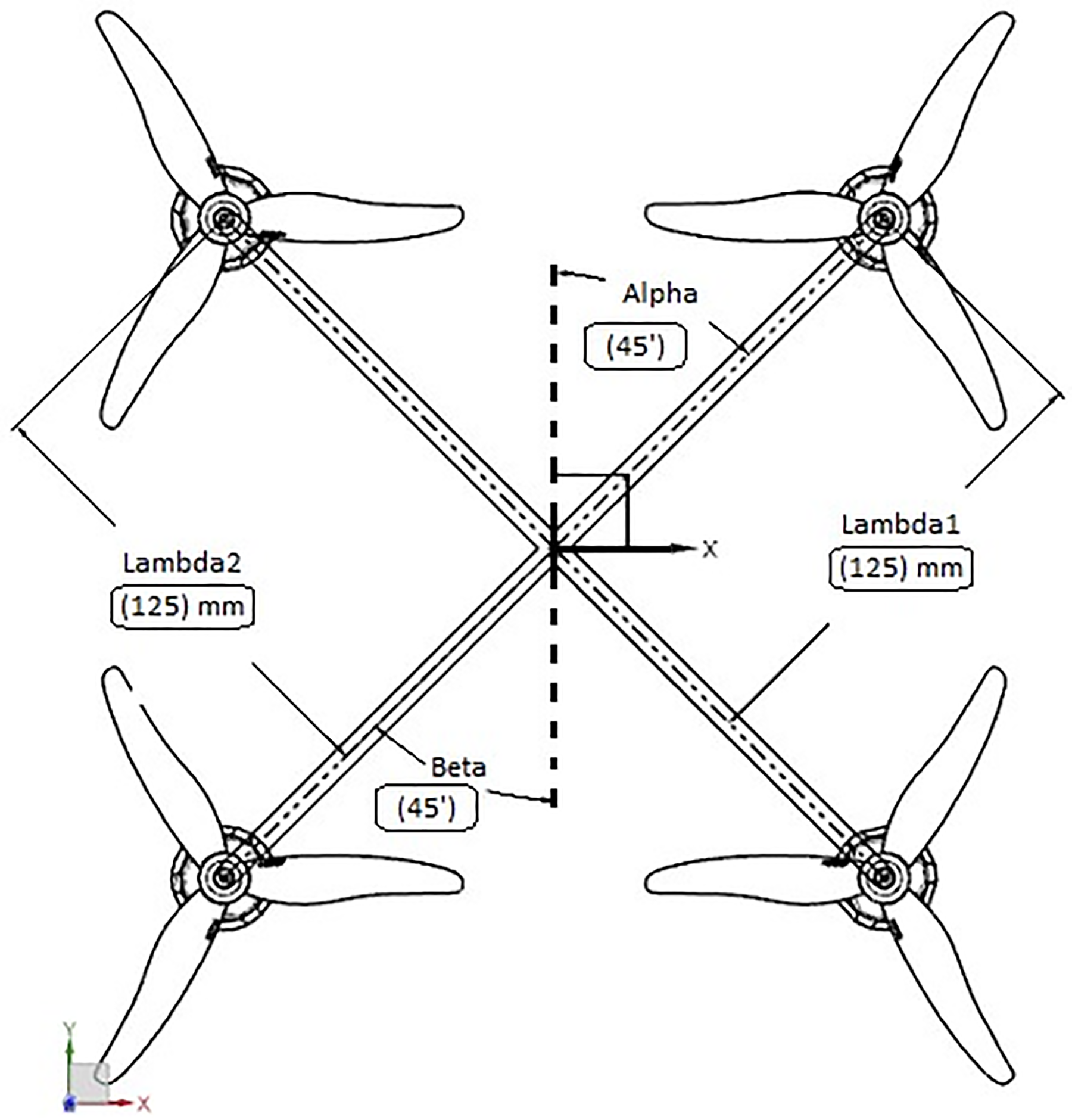
The lambda $(λ)$ length from the centre of gravity means the body’s mass distribution along the axes. Alpha $(α)$ and beta $(β)$ are the angular lengths between the axes (see Figure 2). The mass distributions and angular lengths recall the exact geometrical properties of a racing drone.⁴⁸ Thus, they are stored in a dataset with material features. In the same way, the moments of inertia for data processing are stored for use with MATLAB/Simulink.

Figure 2.

Basic airframe structure.

Now, if motion aims to make the fastest, semicircular and uniform trajectory possible, it depends, if and only if, on the mass distribution $I_{n x} (λ, α, β)$ of the geometric structure or the moment of inertia of the body⁴⁹ which determines the torque of the structure during a curve $(I_{s})$ . Consequently, if the center of gravity of the structure is located at the origin of the reference frame $b o d y f (x, y, z)$ then achieving a change of direction depends mainly on the changes of the roll angular position $- \frac{π}{2} \leq ϕ \leq \frac{π}{2}$ due to the their angle of inclination $(θ)$ and, to a lesser extent due to the position of the yaw angle $- \frac{π}{2} < ψ < \frac{π}{2}$ as usual in a conventional drone.

Thrust force for racing drones

The expression of the thrust force differs from the standard forms.^50–53 It is a coefficient of static test benches. Indeed, the physical and aerodynamic value stays, as discussed in the literature.^54,55,45

Suppose a racing drone aims to fly the fastest horizontal and straight trajectory possible. In that case, it will depend primarily on its pitch angle 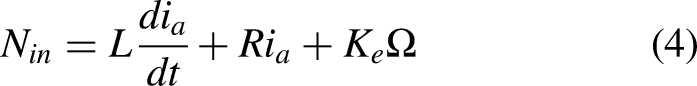$(- π / 2 < θ < π / 2)$ position. If this angle increases, the thrust force must increase too. Thus, the balance of aerodynamic forces is performed, and it will likely hold a straight and level line.

N_{i n} = L \frac{d i_{a}}{d t} + R i_{a} + K_{e} Ω

(4)

The variable

N_{i n}

is the input signal to the motor. It is the magnitude of the nominal voltage times by a normalized input signal. Then, a virtual sensor was located at the propeller’s tip. It is to estimate the rotor speed

(Ω)

. Thus, it is associated with the revolutions per minute of the motor and propeller pace radius. They are both given by the manufacturer. The motor’s electrical characteristics were sourced in the NX motion module (4).

\sum_{i = 1}^{4} T_{n x_{i}} = \sqrt{2 ρ A v_{u} (v_{θ} \cos (θ))^{2} + (v_{θ} \sin (θ) + v_{u})^{2}}

(5)

They are fused with the geometrical properties of the propeller to cause the thrust force (5). The thrust signal is called for each motor. Thus, it provided that the conservation of mass flow rate (

2 ρ A v_{u}

) condition is maintained during stable and level flight. Where

T_{n x_{i}}

is the thrust force for each motor.

The racing drone’s forward speed $(20 \leq v_{θ} \leq 40)$ (m/s) was measured experimentally⁴⁸ and according to its angle of inclination $(θ)$ . Therefore the induced velocity is calculated as follows:

v_{u} = \sqrt{(Ω)^{2} + (v_{θ})^{2}}

(6)

With

v_{u}

as induced velocity.

Trajectory tracking - Control Position

The dynamics of a racing drone are highly non-linear.⁴⁸ It was handled with Matlab design tools. First, the plant was trimmed around the hovering position. Subsequently, it was also linearised as $G (s)$ . Thus, the input signal-angle $ϕ$ in radians and output signal-voltage $V_{a}$ in volts.

G (s) = \frac{ϕ (s)}{V_{a} (s)} = 46858 \cdot \frac{1 - 14.616 \cdot s}{1 + 2 \cdot 0.9 \cdot 152 \cdot s + (152 \cdot s)^{2}}

(7)

The angles and their rate were all steady-state. The airframe speed and position also. Likewise, the drone altitude. Thus, the effects for controller position (x, y) is an underdamped model system. It is with a zero at the origin (7). It has a precision percentage more significant than 92

%

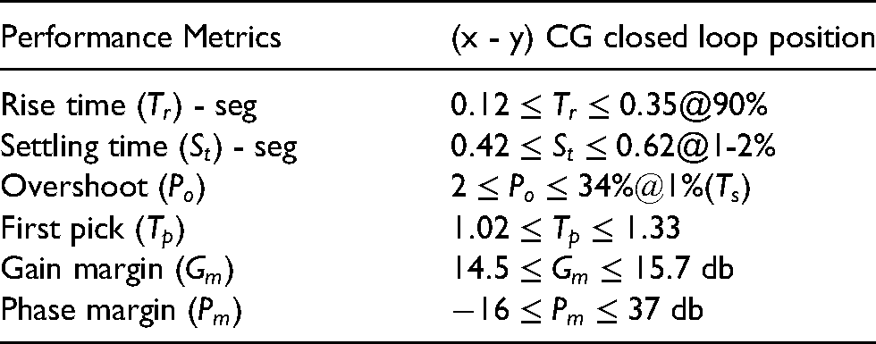
Table 3 shows a range of performance restrictions for a racing drone. Also, the system holds poles in a fit range of metrics. Thus, Figure 3 shows that the contrast between non-linear and linear systems is stable. That way, good pole order meets multiple performance goals. That is, the white area reveals all likely candidate closed-loop poles. In this way, the dynamic of the racing drone is controlled without altering its innate structural design. Taking into account that $w_{f}$ is the damped natural frequency.

Figure 3.

Performance metrics range - (x, y) closed loop.

Table 3.

Time Domain analysis - Racing performance.

Performance Metrics	(x - y) CG closed loop position
Rise time $(T_{r})$ - seg	$0.12 \leq T_{r} \leq 0.35$ @90%
Settling time $(S_{t})$ - seg	$0.42 \leq S_{t} \leq 0.62$ @1-2%
Overshoot $(P_{o})$	$2 \leq P_{o} \leq 34 % @ 1 % (T_{s})$
First pick $(T_{p})$	$1.02 \leq T_{p} \leq 1.33$
Gain margin $(G_{m})$	$14.5 \leq G_{m} \leq 15.7$ db
Phase margin $(P_{m})$	$- 16 \leq P_{m} \leq 37$ db

The Matlab Control System Designer application has been used for multiple concurrent tasks. First, it was used to assess the effect of the gains. Secondly, it was used to catch their behaviour. In addition, this was used to fine-tune the design of the controller structure. In this way, the root locus of the system was conducted. The step responses and the controller effort also.

The process applies to a dynamic model of the non-linear system. It means a closed-loop architecture that needs to be controlled. Those are remade into linear models: It stands for the model’s Zero-Pole-Gain (ZPK). Also, it can be a Transfer Function (TF) of the model. Likewise, into a State Space - Matrix (SS) functions. Thus, they are packed into the Matlab application. At this point, the requirements of the design must be defined (see Table 3). This way, the voltage regulators are continually adjusted (See Figure 3). The process is ended when the desired performance is gained.

The app can be used directly if at least one of the linear models is available. Also, the linear model can be loaded into the design architecture. If not, it is possible to start the PID tuner app directly to design and tune the controllers.

The dynamics of a racing drone were earlier studied experimentally.⁴⁸ Rash accelerations were found. In addition, high speeds in quick times were seen. Due to this and the fact that it is not planned to set high levels of automation, thus, a classic cascade PID control strategy was picked (see Figure 4) for the simulation platform. In this way, the described design process was used. Where $1 F B$ means feedback loop. $D_{m}$ is body mass distribution. Moreover, $F_{T}$ defines the thrust force caused by the system’s motors and propellers’ frequency converters (ESCs).

Figure 4.

Schematic of the control architecture.

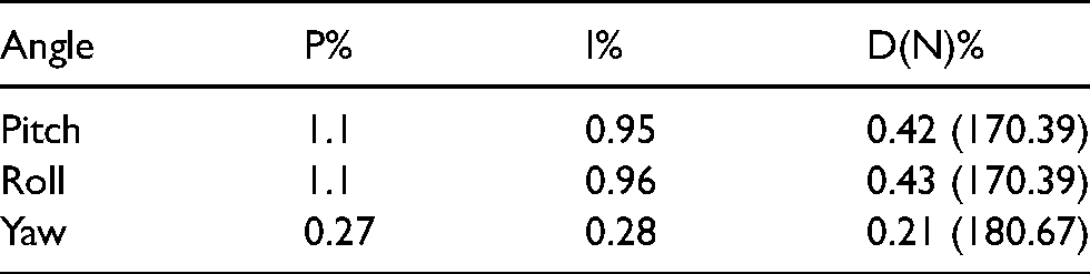
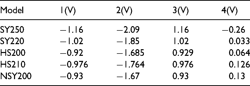
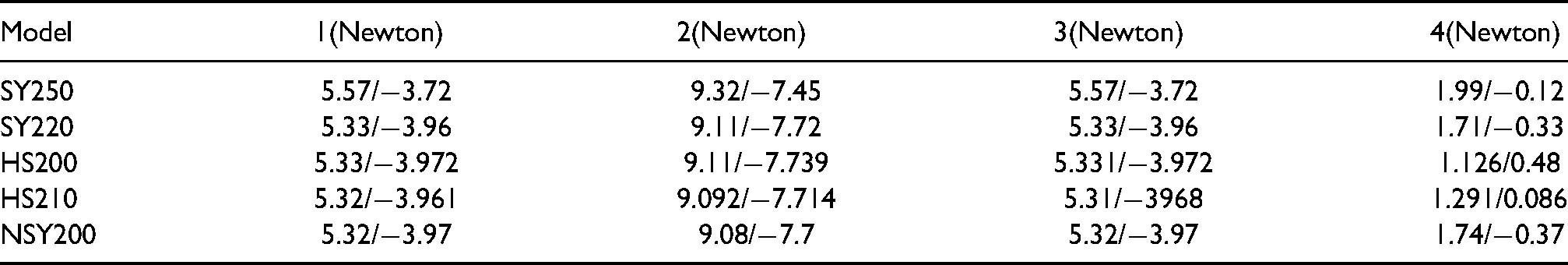
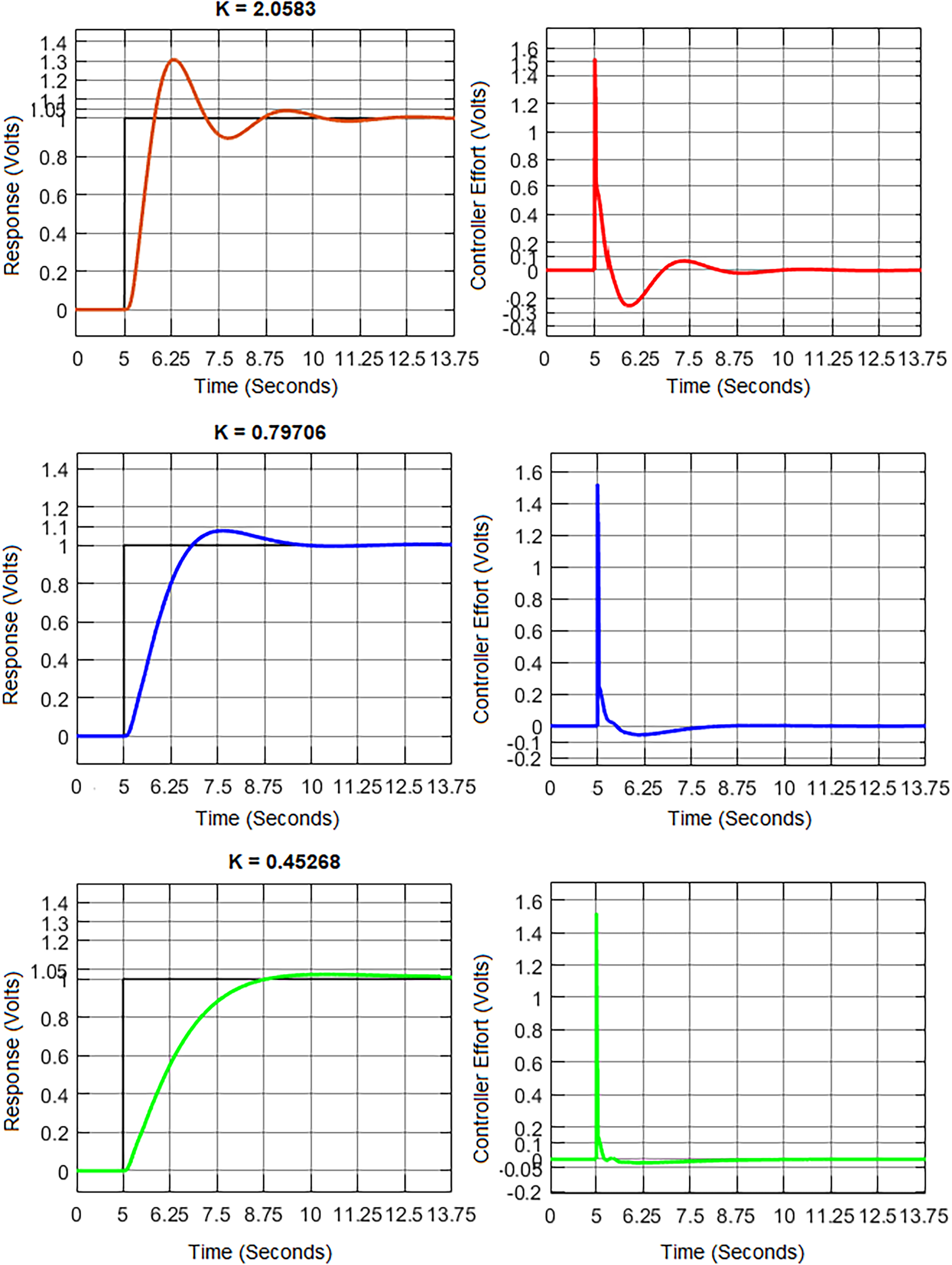
The effect of the three chosen candidate compensators (K) is presented in Table 4. Also, it shows the designed PID controller structure. It is to control the position of the $C G (x, y)$ system after the design method is ended. Further, the system response is shown in Figure 5. Hence, the effort of the position controllers. Note that the compensator has a pole quite far from the origin. It means reasonably fast dynamics. In this way, the range of effort of the controller between the $0.2$ and $2.1$ -volt units is sufficient. The control actions will be adjusted based on a reference model. In addition, it kept within the voltage ranges of the applied references. Thus, the kind of airframes had in the platform is linked to the control effort forced by the specific mass distributions.

Figure 5.

System response and controller effort applying the three designed controllers.

Table 4.

PID controller structure.

$G (s) = \frac{V_{a} (s)}{u (s)}$	Gain K
$K \cdot \frac{(s^{2} + 0.04819 s + 0.03879)}{s (s + 100)}$	2.0583, 0.45268, 0.79706

Trajectory guidance

The international sporting regulations (FAI) do not allow wheelbases ( $λ$ ) greater than 0.3 meters. The most suitable ones vary between 0.2 and 0.25 meters.⁴⁸

(\sqrt{(R e f_{x} (i d x, 1) - x_{s})^{2} + (R e f_{y} (i d x, 2) - y_{s})^{2}}) < 0.25

(8)

Assume that the point

(x_{s}, y_{s})

at the body’s centre of gravity means the drone’s current position. In that case,

R e f_{x y} = (R e f_{x}, R e f_{y})

shows the desired position that needs to be earned. Also, suppose that the subtraction between these two points is less than

0.25

meters, as indicated by the equation 8. In that case, the nose of the drone has to change direction-heading and go to the next point. The international sporting regulations (FAI) do not allow wheelbases greater than 0.3 meters and according to the literature,⁴⁸ the most suitable wheelbases vary between 0.2 and 0.25 meters. Now, if the point

(x_{s}, y_{s})

at the centre of gravity of the body indicates the current position of the drone, then

R e f_{x y} = (R e f_{x}, R e f_{y})

indicates the desired position that needs to be reached. Therefore, if the difference between these two points is less than

0.25

meters, calculated as indicated by the equation 8, then the nose of the drone has to change direction-heading and go to the next point. A new desired angle

(Ψ_{R e f})

or Bearing is calculated. It is for aligning the nose camera of the aircraft with the next point, (9); thus, the nose camera points towards a new desired point.

Ψ_{R e f} = a t a n 2 (z_{d}, y_{d}) - Ψ_{d}

(9)

It is important to note that this form of guidance does not consider tracking policies. The racing drone performs the turn and points directly to the point. That is, this angle regulates the turn limit. Also, the trajectory path takes into account the pilot’s perspective. The racing drone rotates to see the point and steers in a straight line. It allows the behaviour of this kind of drone to be studied more realistically. Thus, the performance of each racing drone can be evaluated on five different trajectories.

Simulation platform experiments

The co-simulation aims to use a typical racing drone airframe design. Also, track the trajectories and guide them around race tracks by waypoints. However, the aim is not to guide the trajectory between points like autonomous racing drones. It is related to the pilots’ point of view. The structure of the racing drone is drawn on the NX CAD module. MATLAB-Simulink will cause the flight trajectory.

Three well-defined sets of airframe models have been recalled.⁴⁸ They are named symmetric (SY), non-symmetric (NSY) and hybrid (HS) geometries. A generic symmetric model has been chosen for the airframe design. Figures 6 to 8 show the setup of the NX CAD model assembly.

Figure 6.

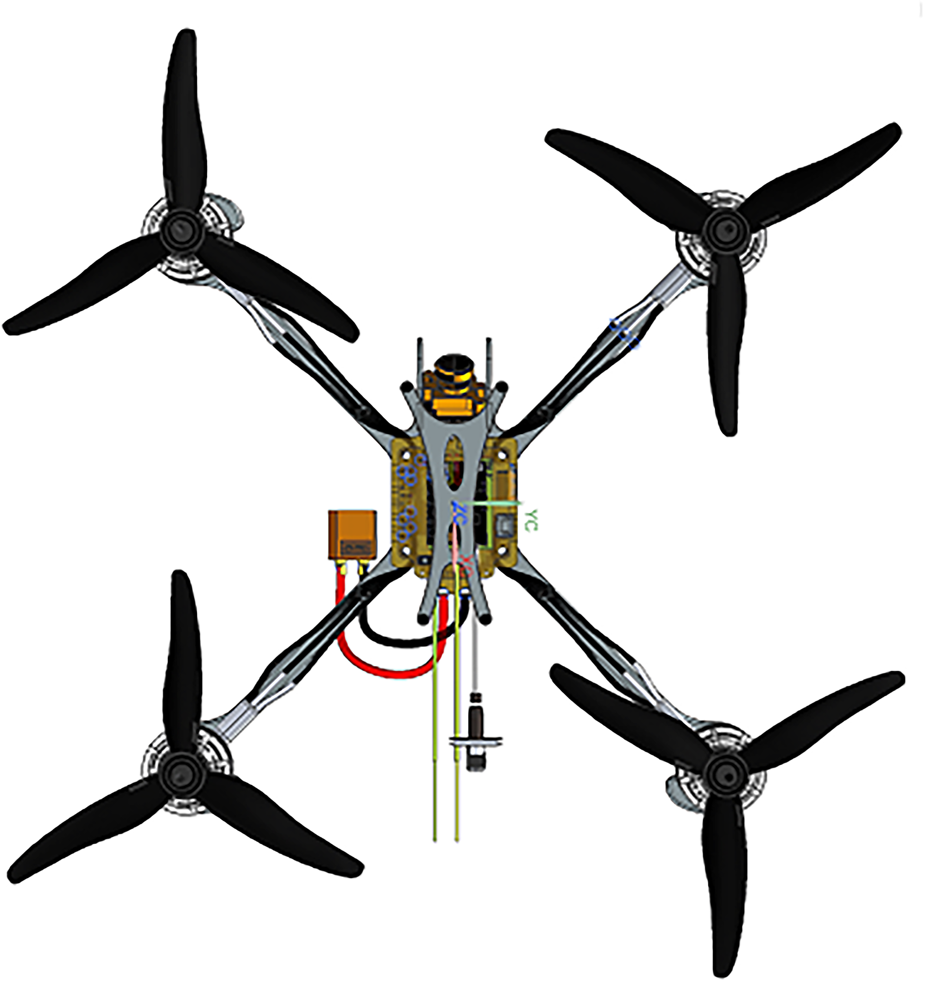
NX CAD part set up / Front view.

Figure 7.

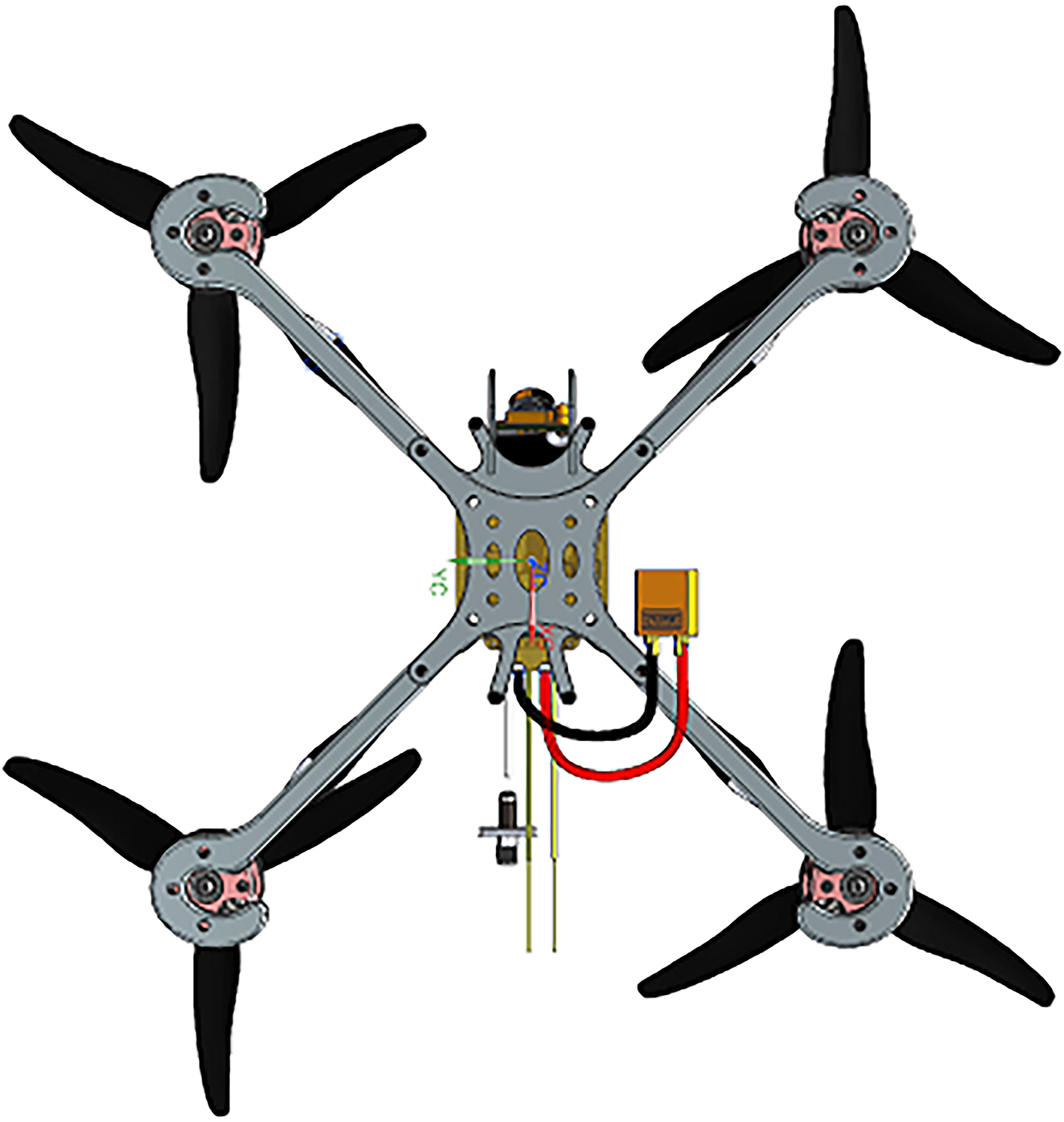
NX CAD part set up / Back view.

Figure 8.

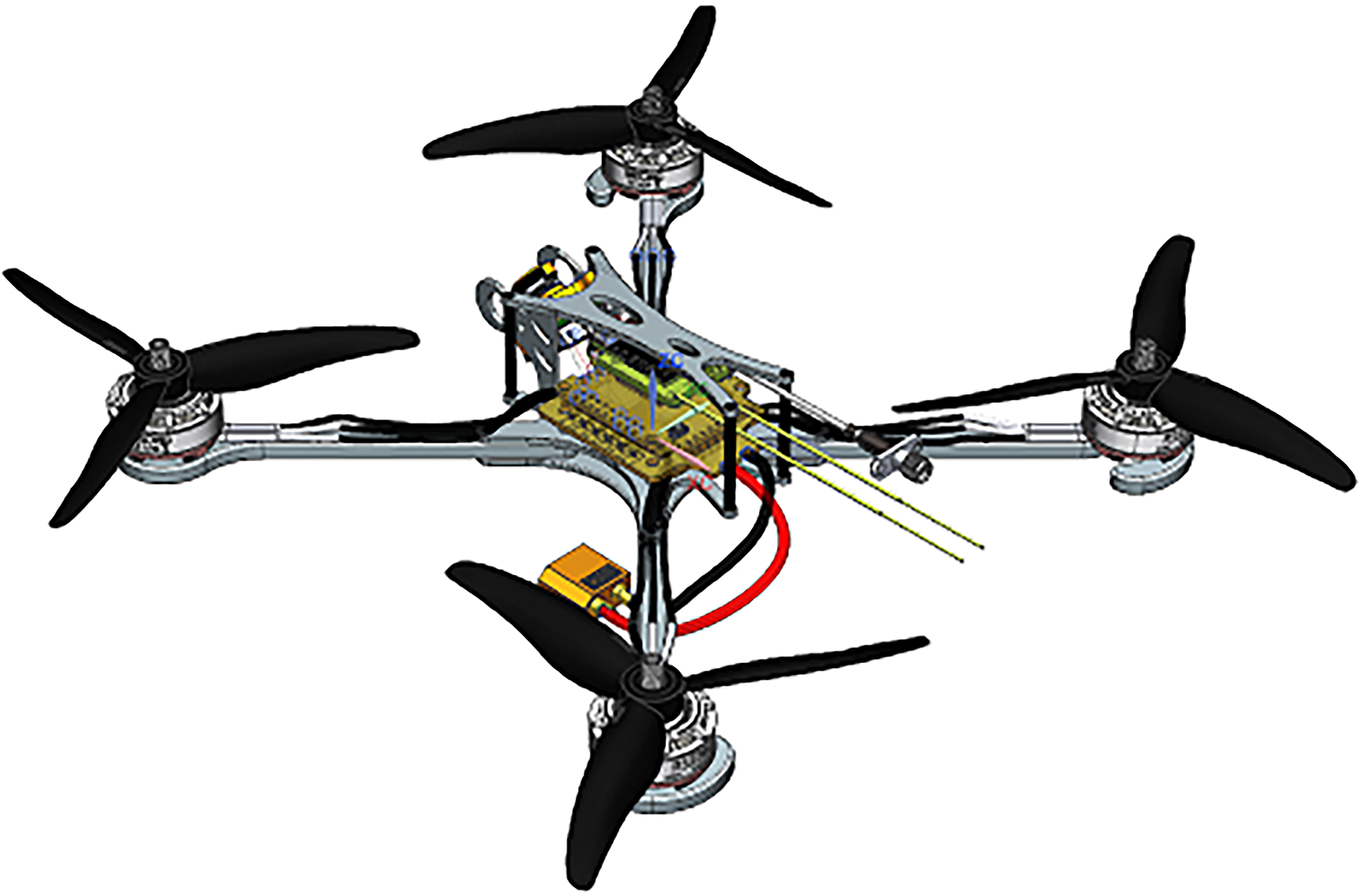
NX CAD part set up / Perspective view.

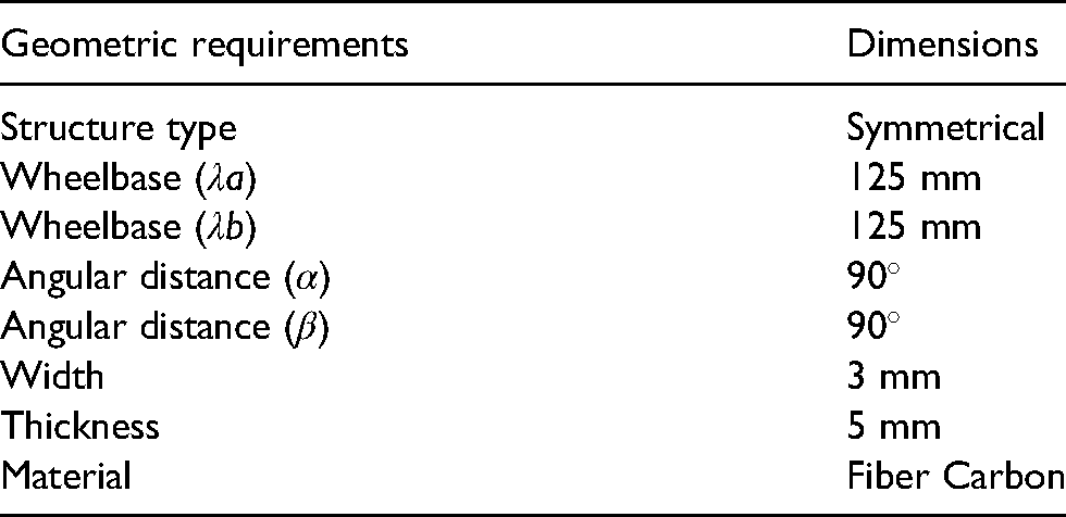
Basic requirements for geometry design are shown in Table 5. It relates to the mathematical expressions of the CAD part sizes. The material features for all parts are assigned in the part module of NX. It is found following the route:

1. \MENU\TOOLS\MATERIALS\ASSIGN MATERIALS

Table 5.

Technical geometric specifications.

Geometric requirements	Dimensions
Structure type	Symmetrical
Wheelbase $(λ a)$	$125$ mm
Wheelbase $(λ b)$	$125$ mm
Angular distance $(α)$	$90^{\circ}$
Angular distance $(β)$	$90^{\circ}$
Width	3 mm
Thickness	5 mm
Material	Fiber Carbon

The material created for the airframe structure is an intermediate stiffness carbon fibre (IM). It has a low modulus of over 100 GPa. The tensile strength is greater than 3 GPa. With a density of 2 $g / c m^{3}$ and elongation of 1%. The package has 3000 thousand filaments (3K). The elastic modulus is also shown in Figure 9.

Figure 9.

Material characteristics.

Suppose it is required to access the body mass distribution analysis and all moment-related results from the NX platform. In that case, they should be found in excel file format following the route:

1. \MENU\ANALSYS\GEOMETRIC PROPERTIES

2. \MENU\ANALSYS\ADVANCED MASS PROPIERTIES

The effects of the geometric features are shown in Table 6. A script from MATLAB records the whole excel database. Thus, it sends the needed data to a Simulink block. A simulation stage is built to generate the thrust force signal. It is built from the NX motion module. All physical features of the structure are inherited from the CAD module.

Table 6.

Results of body mass distribution.

Physical properties	Results (kg-mm)
Density	$5.39944 E - 06$ $(k g / m m^{3})$
Volume	$69636.4721$ $(m m^{3})$
Mass	$0.375997845$ $(k g)$
Center of Mass	Body
$X_{c}$	$0.000436526$ $(m m)$
$Y_{c}$	$10.89804522$ $(m m)$
$Z_{c}$	$18.58603971$ $(m m)$
Moments of Inertia	Body
$I_{x x}$	$2046.459543$ $(k g / m m^{2})$
$I_{y y}$	$2077.889524$ $(k g / m m^{2})$
$I_{z z}$	$4062.291704$ $(k g / m m^{2})$

In the Figure 10 it is possible to observe the motion simulation scenario. Note that the yellow and black colours define the links to be joined. The rotation axis (Z) arrow represents the output force and direction. A revolute joint connects the motor and propeller. Also, they are connected to the airframe arm by a fixed joint. The degrees of freedom of the structure is defined by nine links, four joints per revolution and five fixed joints. Thus, it simulates the motion of motors and propellers. To start the motion simulation, the input to the system is a step function. It emulates the throttle lever positions starting at 50% of the total travel. This signal is multiplied by the nominal voltage. In this way, it obtains its magnitude and direction of rotation. A motion sensor is located at the propeller’s tip to store its RPM.

Figure 10.

NX Motion simulation environment.

It is also possible to see two brown arrows in Figure 10. The vertical arrow on the Z-axis means the output force and direction. Also, the arrow around the Z-axis shows the direction of rotation. The output by each motor is a normalised signal. It emulates the thrust force for 50, 60, 75, 90 and 100% of the throttle lever travel, and its magnitude is stored in a force container.

The FAI sporting code suggests using 4s up to 6s batteries. So, the maximum voltage allowed in a racing competition is about 17-23 volts. In addition, the propeller lengths are up to around 5.9 inches. Also, the magnitudes required for the thrust force to be modelled are listed in Table 7. Likewise, these conditions match with a set of earlier assessed electronic pieces.⁴⁸

Table 7.

Thrust force requirements.

Coefficients and variables	Magnitude
Nominal Voltage	$14.5 \leq v o l t s \leq 16.11$
Characteristic area (A)	$0, 053$ $(m^{2})$
Rotor speed $(Ω)$	25253 $(r e v / m i n)$
Forward speed $(v_{θ})$	37,5 $(m / s)$
Tilt angle $(θ)$	55 $d e g r e e s$
Propeller length	51 $i n c h$
Propeller pitch	47 $d e g r e e s$

The parameters to link with Matlab-Simulink are in Table 8. The solver algorithm that holds all the execution routines is called Recurdyn. The set of RMD, MSG and RPLT files make up the solver.

Table 8.

NX parameters.

General parameters	Communication feature
Solver NX	Recurdyn
The solver data set	RMD
Record of the solving process	MSG
Animation data	RAD
Graphing Data	RPLT
Solver Parameters	Customizable
Dynamics	Motion simulation
Initial step	1E-006
Error tolerance	0.001
Numerical damping	1
Max iteration	50
Co-simulation	Unigraphics NX 11
Sampling Time	0.001 seg
Analysis type	Control/dynamics
Simulation time	150 seg
Steps	15000

A user-definable block (s-function) is used to load the NX motion dynamic parameters to Matlab. This function is called by the name version of NX that is running. A successful link should result in an NX Simulink block, as in Figure 11.

G (s) = \frac{T h r u s t (s)}{V_{a} (s)} = \frac{9.0519}{1 + 0.060538 \cdot s}

(10)

Figure 11.

NX Thrust Dynamics.

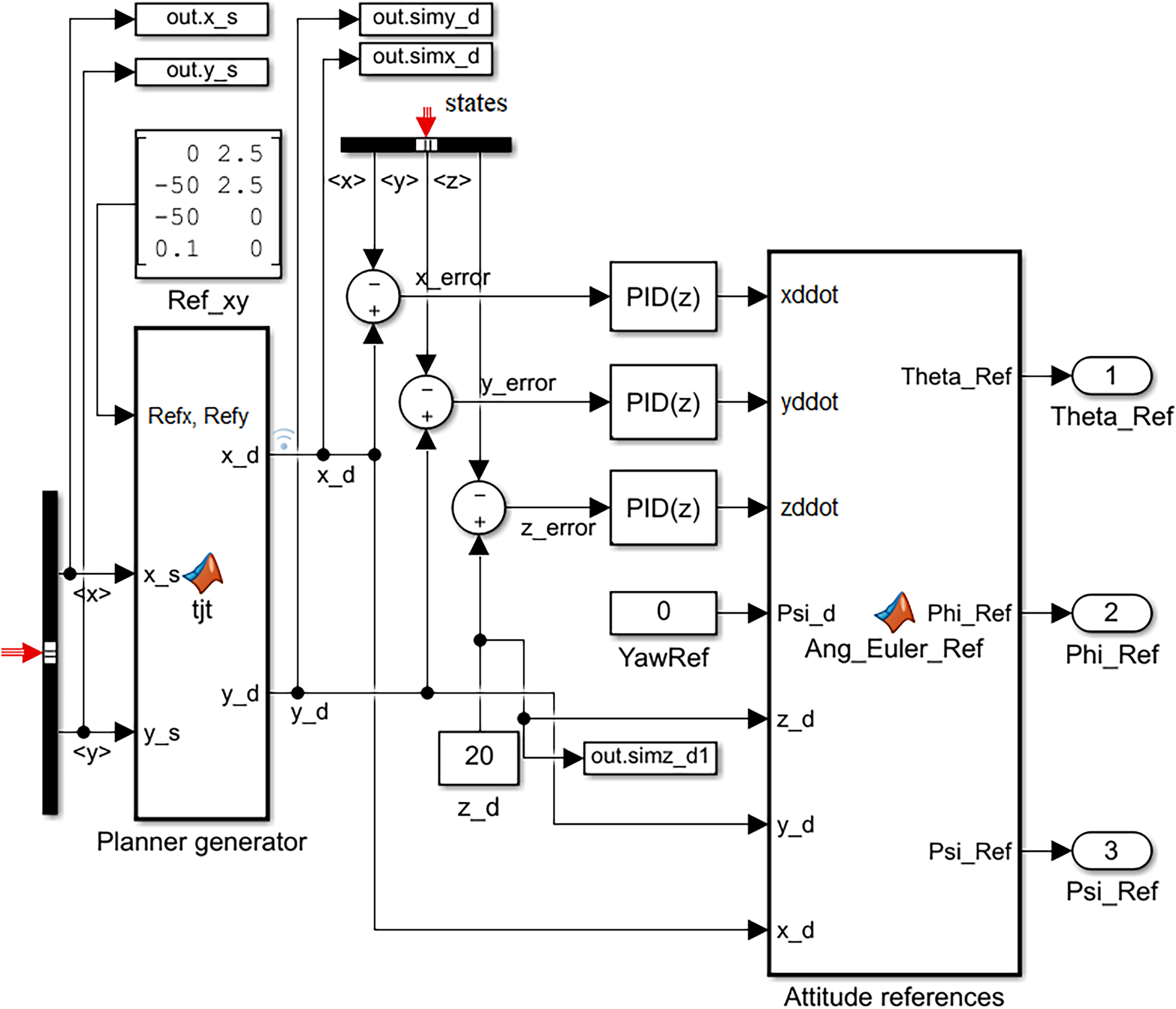
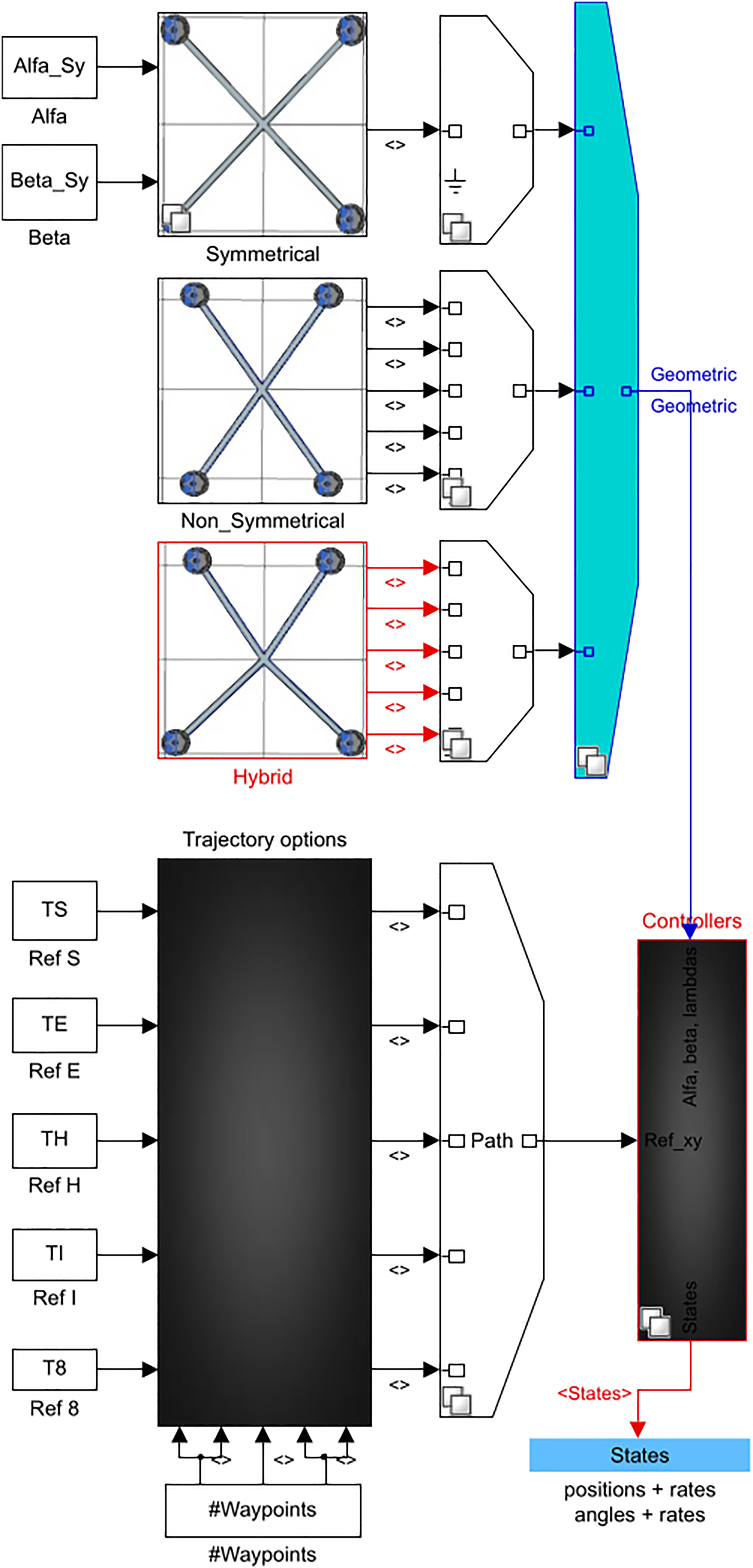
A transfer function (10) identifies the NX plant. In this way, tune the control parameters in Simulink. Note that the thrust is Newton-units. Also, $V_{a}$ is Volts-units. The output thrust forces are computed with the Airframe torque (3). Thus, to estimate the values of the translational motion of the body. Also, the angular accelerations. It is a result of a rotation of the pitch and roll angles.

The diagram shows (see Figure 12) the tools used to realise the design. Also, it shows how they interact with each other. The translational accelerations $(x d d o t, y d d o t)$ were defined. Also, the Euler angles rotations ( $P h i d d o t$ , $T h e t a d d o t$ , $P s i d d o t$ ). The settings of both motions in Simulink can be seen in the annexes (see figures 21 to 25). Thus, if all initial conditions are set to zero to define the integrals, the current state of the drone position will be defined by the points $(x_{s}, y_{s}, z_{s})$ .

Figure 12.

Control design strategy.

The track layout is a matrix with reference points $R e f_{x y} = (R e f_{x}, R e f_{y})$ . Suppose these reference points are subtracted from the points ( $x_{s}, y_{s})$ . In that case, the trajectory is generated by (8), and the result is the destination points $(x_{d}, y_{d})$ .

The subtraction between the destination points and the current position of the centre of gravity $(x, y)$ tracks the trajectory (see Figure 13). In this way, it controls the Drone’s position. The desired points are used by attitude control as references. Thus, to estimate Euler angles and correct slight deviations during straight trajectories. In addition, a sub-cascade of angular speed control has been included, as shown in Figure 14. Also, note in this figure that the controlled or commanded signals mixer is at the end of the entire control loop. Those are the inputs to the NX thrust dynamic block (see Figure 11).

Figure 13.

Guidance and trajectory tracking.

Figure 14.

Angular rate and attitude control.

The result of the co-simulation is successful (Figure 15). Points 1, 2, 3 and 4, labelled in Figure 15, indicate the points on the rectangular trajectory that the drone has travelled. Thus, waypoints 12 – 34 are 2.5 metres, and 23-41 are 50 metres. The directional components of the trajectory have been calculated. It is to confirm that the drone points with the nose towards the direction of the second point, as seen in Figure 16. It simulated the perspective of the first-person view (FPV). The red arrows show the direction of the nose of the drone. For this experiment, the simulation flow starts at 0.0 seconds, and the stop time is between 300 and 700 seconds in Simulink. The type of solver used is called variable-step.

Figure 15.

Typical trajectory of a racing circuit.

Figure 16.

Video camera pointing towards the target point – for first person view - FPV.

The sample time in Simulink was set to 0.01 seconds. The Dormand-prince solver (ODE45) was used to run de simulation. In contrast, the Forward Euler method was used to assess control gains. It is a numerical approach to the Runge-Kutta methods.

The studied motion dynamics related to Figure 17 were linked to a rectangular flight trajectory. It is through waypoints 1, 2, 3 and 4, as shown in Figure 15. Note that waypoints 12 and 34 connect to sectors with tight turns. So, waypoints 23 and 41 to straight trajectories.

Figure 17.

Dynamic behaviour of the models according to the effort of the controllers and the thrust force requested.

The gains of the voltage regulators used are the default ones (see Tables 9 to 11). Where $N$ is a filter coefficient to implement the derivative action and avoid improper transfer functions.

Table 9.

Attitude controller default values.

Angle	P%	I%	D(N)%
Pitch	13.77	5.23	0.71 (17.37)
Roll	19.2	6	3.3 (124.6)
Yaw	3.66	2.69	0 (6.68)

Table 10.

Rate controller default values.

Angle	P%	I%	D(N)%
Pitch	1.1	0.95	0.42 (170.39)
Roll	1.1	0.96	0.43 (170.39)
Yaw	0.27	0.28	0.21 (180.67)

Table 11.

Position controller default values.

Angle	P%	I%	D(N)%
Pitch	1.6	2.03	0.2 (22.53)
Roll	2	4.5	7.5 (84.45)
Yaw	2.7	12.5	1.0 (12.82)

Figure 17 shows all the kinds of racing drones⁴⁸ included in the platform. It considers the mass distribution of all models. In addition, the features of the electronic components are in Table 7. It also shows the capacity of the effort made by the controllers. It is due to the thrust force demanded by the motors. It is over a square trajectory. However, studying the dynamics of racing drones on five diverse trajectories is doable doable (See Figures 19, 26, 27, and 28 in annexes section). These are usual trajectories performed in an FPV competition.

Figure 17 contains ten graphs from the letter a to e. The thrust force required by the motors is shown on the right-hand side of Figure 17. The effort the regulators made to meet the requested force is shown on the left-hand side. The grey arrows and the horizontal lines on the left-hand side of Figure 17 show the time per lap for each model—also, the maximum effort made by the controllers through the trajectory. A straightforward graph is placed in descending order. It means that at the top of Figure 17 are placed the models with the most extensive Wheelbase ( $λ$ ) and heaviest weights. Thus, the models with the shortest wheelbase ( $λ$ ) and most minor weights are at the bottom. In addition, each of the single graphs includes a symmetric (SY), a non-symmetric (NSY) and a hybrid (HS) airframe model.⁴⁸ In outlook, it can be seen how the time per lap and the effort achieved by each controller decrease as the structures reduce their wheelbase $(λ)$ and weight. In a word, note how the grey arrows increase in length as the graphs descend. Also, note how the horizontal lines at each waypoint ascend. In graph, a(1), note how the controller’s effort at waypoint 2 exceeds two volts. While in graph b(1), the effort is on the two volt-line, in graph c(1), it is above two volts. Also, note that symmetrical structures (SY) have the lowest lap times among all models. It is irrespective of the wheelbase $(λ)$ and weight. Thus, note the SY210 (see graph d(1)). Also, SY220 (see graph c(1)). Likewise, SY230 (see graph b(1)) model keeps the dynamic behaviour. In contrast, the SY250 (see graph a(1)) model achieves a slight difference, being the heaviest. This behaviour is only compared to the lighter SY200 (see graph e(1)). Thus, these models’ motors, propellers and batteries achieve the highest thrust forces. It is between 9.3 and 7.7 newtons in a roll turn, as seen on the right side of the figure. The quantities of the simulations are summarised in Tables 19 to 27 in the annexes section.

Tables 12 to 14 are for the models with outstanding dynamic behaviour. They show the quantities of the flight test simulation. Note that peaks of effort controller appear on tight turns (waypoints 1-2 and 3-4). Regardless, the maximum thrust forces are earned. In contrast, those remain constant on straight trajectories (waypoints 2-3 and 4-1). It is then tracked that the non-symmetric (NSY) has slightly different dynamics on tight turns. Likewise, hybrid (HS) models. However, the mass distribution of HS models allows higher force than the NSY. Although per similar pieces of effort offered by controllers on the straight trajectory. The highest thrust on turns is around 9.3 and 7.5-newton units. While in straight trajectories is nearly 0.9 and 0.7. Graph a2 shows the heaviest models. Note that the SY voltage controllers cover the highest thrust demand requested by the motors. Also, that model reaches the highest performance. Even the lightest model falls short of this performance (see graph e(2)).

Table 12.

Lap-times performance through waypoints.

Model	1(s)	2(s)	3(s)	4(s)
SY250	154.66	162.33	389.1	396.7
SY220	154.66	162.31	394.4	394.5
HS200	187.8	195.4	427.9	429.7
HS210	188.7	196.4	436.7	444.4
NSY200	220.5	228.1	479.9	487.5

Table 13.

Effort controller performance through waypoints.

Model	1(V)	2(V)	3(V)	4(V)
SY250	$-$ 1.16	$-$ 2.09	1.16	$-$ 0.26
SY220	$-$ 1.02	$-$ 1.85	1.02	0.033
HS200	$-$ 0.92	$-$ 1.685	0.929	0.064
HS210	$-$ 0.976	$-$ 1.764	0.976	0.126
NSY200	$-$ 0.93	$-$ 1.67	0.93	0.13

Table 14.

Thrust controller performance through waypoints.

Model	1(Newton)	2(Newton)	3(Newton)	4(Newton)
SY250	5.57/ $-$ 3.72	9.32/ $-$ 7.45	5.57/ $-$ 3.72	1.99/ $-$ 0.12
SY220	5.33/ $-$ 3.96	9.11/ $-$ 7.72	5.33/ $-$ 3.96	1.71/ $-$ 0.33
HS200	5.33/ $-$ 3.972	9.11/ $-$ 7.739	5.331/ $-$ 3.972	1.126/0.48
HS210	5.32/ $-$ 3.961	9.092/ $-$ 7.714	5.31/ $-$ 3968	1.291/0.086
NSY200	5.32/ $-$ 3.97	9.08/ $-$ 7.7	5.32/ $-$ 3.97	1.74/ $-$ 0.37

Note that the thrust forces for the NSY and HS models are similar on the trajectories. However, as the weights decrease, shorter lap times are earned. Also, the time gap and weight of each airframe decrease. Thus, the ability to fulfil the raised thrust on straight trajectories is proportional to the model’s weight. However, it is limited by the speed controller (ESC). It must often respond to speed shifts. In this way, it limits the amount of acceleration earned on straight trajectories. It is possible to attribute the performance in tight turns to the geometry aspect ratio (i.e. $λ, α$ and $β$ ). Due that acceleration is the effect of rash shifts in turns. However, it is limited by the controller’s ability to meet the requested thrust demand. Thus, it is not attributable to speed shifts.

Setting up relevant control actions is critical. It should be according to the geometric shape kind of the airframes. Thus, the dynamic operating range has to be shrunk. Proper action control allows taking the edge of the mass distributions of the airframes. Thus, reach the dynamic behaviours described in the literature.⁴⁸ Else, the control system tends to prefer symmetrical airframes (SY). Suppose the likeness of the controller stresses is considered. Also, mass distribution is taken into account. In this case, the SY stands out. It is due to its long arm and inertia effects. Unlike, the HS model does not take the edge of its shape. Thus, there is no proof of a racing leap. It is vital to handle the controller gains suitably for a specific trajectory.

How to set up multiple experiments

The platform consists of five blocks of variants. It is to handle the simulation process: Gray variant block stores the trajectory control loops. Black variants stored the system guidance. Thus, three variant blocks hold the geometric features of each airframe (SY, NSY and HS) (See Figure 18).

Figure 18.

Simulation Platform for racing airframes.

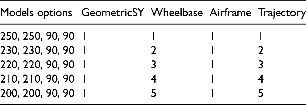
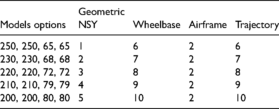
Choosing the control path before running the simulation is required. The airframe shape should be specified. Also, the wheelbase has to be selected. Likewise, the communication ports and the platform must be updated. For this, variables should be writ in the Matlab window. It is set in the annexes section. All feasible geometric has already been validated on the platform. Thus, the control path is defined in Tables 15 to 17. The platform offers five standard FPV trajectories. Table 18 defines the path to be selected. In addition, Figure 19 shows another kind of trajectory of a racing drone. The vertical black lines define the usual obstacles of an FPV competition. To apprehend the trajectory realistically, thus, the control point is placed in the centre of the obstacle. When the nearness to the point is less than 0.25 mm, the pilot turns the drone, and it goes to the next obstacle. These can be applied to each kind of drone chosen. Thus, the dynamics of the model may be studied as a function of the stress on the controllers. Also, the forces interacting on the picked trajectory could be studied.

Table 15.

Options airframes Symmetrical structures.

Models options	GeometricSY	Wheelbase	Airframe	Trajectory
250, 250, 90, 90	1	1	1	1
230, 230, 90, 90	1	2	1	2
220, 220, 90, 90	1	3	1	3
210, 210, 90, 90	1	4	1	4
200, 200, 90, 90	1	5	1	5

Table 16.

Options airframes Non - Symmetrical structures.

Models options	Geometric NSY	Wheelbase	Airframe	Trajectory
250, 250, 65, 65	1	6	2	6
230, 230, 68, 68	2	7	2	7
220, 220, 72, 72	3	8	2	8
210, 210, 79, 79	4	9	2	9
200, 200, 80, 80	5	10	2	10

Table 17.

Options airframes Hybrid structures.

Models options	Geometric HS	Wheelbase	Airframe	Trajectory
250, 250, 65, 90	1	11	3	11
230, 230, 68, 90	2	12	3	12
220, 220, 72, 90	3	13	3	13
210, 210, 79, 90	4	14	3	14
200, 200, 80, 90	5	15	3	15

Table 18.

Trajectory options.

Trajectories	Guidance	Path
Square	1	1
E letter	2	2
H Letter	3	3
I letter	4	4
Cross	5	5

Figure 19.

Trajectory options – Cross.

The control path will be highlighted in black if the above commands are correctly typed. The platform will be ready to run a simulation. The kind of airframe preloaded on the platform has been carefully picked. It fits the report raised about racing drones.⁴⁸ Thus, suppose that the controllers require a custom fit. Likewise, the reference generator needs to be edited. In those cases, all airframe choices have a unique control system. It can be found within the grey variant block. They also follow the control system shown in Figure 4.

Conclusions

The platform is open in Matlab Central for file sharing.⁵⁶ It is planned from the racing driver’s view. Still, it even offers a broad option of approaches. It is feasible to get distinct kinds of airframes. It means to asses the dynamic performance on unlike trajectories. In addition, sort of situations can be handled. These are tied to aerodynamic or autonomous control problems. Also, to study topics linked to machine learning. All the toolboxes offered by Simulink can be used.

The platform offers to check all design features. It means each geometric option can be studied apiece. It has 15 kinds of known airframes. In addition, it offers the option of adjusting all the control loops based on need. Thus, the motion of the drones can be linked to the accelerations reached on the trajectories. It is an open platform that lets in new updates. That is, it can be boosted to acquire data from vision sensors. Also, obtain data in real-time or for hardware uses.

All airframe models inside the platform are variants of the system. Suppose the goal is to optimise the controllers. In that case, each variant can evolve a system model. Thus, adaptive control methods can be offered. Now, suppose the goal is to optimise the geometric features. It is for studying the trajectories and the controllers’ efforts. In that case, all airframe sizes are script functions or parametric equations.

The aim is to study the dynamics of racing drones. Thus, the platform handles the equations of motion in a certain way. In addition, it shows a cascaded PID control for all model variants. Since access to the blocks is open. Thus, it links quickly to any design application (MOD). Likewise, the control scheme is elastic to any case. In addition, the geometric options are ample, allowing racing aerodynamics to be studied. Thus, they can be optimised for distinct trajectories. It makes the platform a flexible design tool.

Earning high performance in demanding situations is a challenge. It needs design goals beyond a classic machine’s performance measures. High dynamic motion, such as that of racing drones, is a sample. Thus, it ought to be handled gradually. Control methods have already been broadly learned. Also, techniques have expanded at the same time. Thus, this study has focused on the kinds of airframes bound to the effort they require from controllers.

The CAD design module allows a high definition of the airframes. This way, a precise estimation of the moments of inertia was aimed. In addition, motion simulations added a degree of exactness. The motors and propellers were also drawn using the CAD module. It allows a proper model of the motor dynamics. That is the motion of the propellers tied to the airframes. Thus, the motion app attaches the features of the model. Likewise, it lessens the computational load in Simulink. Estimating the thrust force outside Matlab seeks a drop in the simulation time. In addition, this streamlines the design flow.

Supplemental Material

sj-pdf-1-mav-10.1177_17568293221143785 - Supplemental material for Co-simulation platform for geometric design, trajectory control and guidance of racing drones

Supplemental material, sj-pdf-1-mav-10.1177_17568293221143785 for Co-simulation platform for geometric design, trajectory control and guidance of racing drones by J.M. Castiblanco Quintero, S. Garcia-Nieto, R. Simarro and J.V. Salcedo in International Journal of Micro Air Vehicles

Footnotes

Acknowledgements

This work was partially supported by proyect PID2020-119468RA-I00 funded by MCIN/AEI/10.13039/501100011033.

Declaration of conflicting interests

The author(s) declared no potential conflicts of interest with respect to the research, authorship, and/or publication of this article.

Funding

The author(s) disclosed receipt of the following financial support for the research, authorship, and/or publication of this article: This work was partially supported by proyect PID2020-119468RA-I00 funded by MCIN/AEI/10.13039/501100011033.

ORCID iDs

J.M. Castiblanco Quintero

S. Garcia-Nieto

J.V. Salcedo

Supplemental material

Supplementary material for this article is available online.

References

Cañas

Perdices

García-Pérez

et al. A ros-based open tool for intelligent robotics education. Appl Sci 2020; 10: 7419.

Caterino

Greco

D’Ambra

et al. Simulation techniques for production lines performance control. Procedia Manuf 2020; 42: 91–96.

Nayebi

Meraji

Shamaei

et al. Xmulator: a listener-based integrated simulation platform for interconnection networks. In First Asia International Conference on Modelling & Simulation (AMS’07). IEEE, pp. 128–132.

Silano

Iannelli

. Crazys: A software-in-the-loop simulation platform for the crazyflie 2.0 nano-quadcopter. In Robot Operating System (ROS). Springer, 2020. pp. 81–115.

Grieco

Iacovelli

Boccadoro

et al. Internet of drones simulator: Design, implementation, and performance evaluation. arXiv preprint arXiv:220313710, 2022.

Jin

. Uav simulator-based simulation of flight control system. In 2009 International Workshop on Intelligent Systems and Applications. IEEE, pp. 1–4.

Carnieletto

Ferrando

Teso

et al. Italian prototype building models for urban scale building performance simulation. Build Environ 2021; 192: 107590.

Reigeluth

Schwartz

. An instructional theory for the design of computer-based simulations. J Comp Based Instr 1989; Volume 16: 1–10.

Zheng

Wang

Liu

. Stochastic optimization for unit commitment—a review. IEEE Trans Power Syst 2014; Volume 30: 1913–1924.

10.

Kleijnen

. Design and analysis of simulation experiments. In International Workshop on Simulation. Springer, pp. 3–22. 2018; Volume 231.

11.

Luo

Yan

et al. Autonomous detection of damage to multiple steel surfaces from 360 panoramas using deep neural networks. Comput-Aided Civ Infrastruct Eng 2021; Volume 36: 1585–1599.

12.

Fiandrino

Capponi

Cacciatore

et al. Crowdsensim: a simulation platform for mobile crowdsensing in realistic urban environments. IEEE Access 2017; Volume 5: 3490–3503.

13.

Brox

Sánchez-Solano

del Toro

et al. Cad tools for hardware implementation of embedded fuzzy systems on fpgas. IEEE Trans Ind Inf 2012; Volume 9: 1635–1644.

14.

Mishchenko

. Exploring the cad model of the manipulator using cad translation and simscape multibody. In E3S Web of Conferences, volume 279. EDP Sciences, p. 03014.

15.

D’Silva

Sundaram

D’Ambrosio

. Co-simulation platform for diagnostic development of a controlled chassis system. SAE Transactions 2006; Volume 115: 498–507.

16.

Khan

MTH

Rezwana

. A review of cad to cae integration with a hierarchical data format (hdf)-based solution. J King Saud Univ-Eng Sci 2021; Volume 33: 248–258.

17.

Cekus

Posiadała

Warys

. Integration of modeling in solidworks and matlab/simulink environments. Arch Mech Eng 2014; Volume 61(1): 57–74.

18.

Grau

Bolea

Sanfeliu

. Cad-based approach for identification of uavs. In MATEC Web of Conferences, volume 291. EDP Sciences, p. 01004.

19.

Gujarathi

. Parametric cad/cae integration using a common data model. J Manuf Syst 2011; Volume 30: 118–132.

20.

Deng

Lam

Tor

et al. A cad-cae integrated injection molding design system. Eng Comput 2002; Volume 8: 80–92.

21.

Vinodh

. Environmental conscious product design using cad and cae. Clean Technol Environ Policy 2011; 13: 359–367.

22.

Ali

Chowdary

Gonzales

. An integrated design approach for rapid product development: A case study through application of reverse engineering, re-engineering and fast prototyping tools. Journal of Engineering, Design and Technology 2013; Vol 11(No2): 178–189.

23.

Berselli

Bilancia

Luzi

. Project-based learning of advanced cad/cae tools in engineering education. Int J Interact Des Manuf (IJIDeM) 2020; 14: 1071–1083.

24.

Gordon

Ruff

Kumar

. Simulating quadcopter dynamics using imported cad data. In AIAA Modeling and Simulation Technologies (MST) Conference. p. 4735.

25.

Ben Ayed

Massaoudi

Alshaya

et al. System-level co-simulation for embedded systems. AIP Adv 2020; 10: 035113.

26.

Dani

Dorle

et al. Modelling and co-simulation of a two-speed transmission for a three-wheel electric delivery vehicle. Technical report, SAE Technical Paper, 2021.

27.

Chen

et al. Co-simulation of complex engineered systems enabled by a cognitive twin architecture. Int J Prod Res 2021; 1–22.

28.

Mellinger

Shomin

Michael

et al. Cooperative grasping and transport using multiple quadrotors. In Distributed autonomous robotic systems. Springer, 2013. pp. 545–558.

29.

Desbiens

Cutkosky

. Landing and perching on vertical surfaces with microspines for small unmanned air vehicles. J Intell Robot Syst 2010; 57: 313.

30.

Fink

Michael

Kim

et al. Planning and control for cooperative manipulation and transportation with aerial robots. Int J Rob Res 2011; 30: 324–334.

31.

Mellinger

Shomin

Kumar

. Control of quadrotors for robust perching and landing. In Proceedings of the International Powered Lift Conference. pp. 205–225.

32.

Mellinger

Kumar

. Minimum snap trajectory generation and control for quadrotors. In 2011 IEEE International Conference on Robotics and Automation. IEEE, pp. 2520–2525.

33.

Kushleyev

Mellinger

Powers

et al. Towards a swarm of agile micro quadrotors. Auton Robots 2013; 35: 287–300.

34.

Turpin

Mohta

Michael

et al. Goal assignment and trajectory planning for large teams of interchangeable robots. Auton Robots 2014; 37: 401–415.

35.

Samadikhoshkho

Ghorbani

Janabi-Sharifi

. Modeling and control of aerial continuum manipulation systems: A flying continuum robot paradigm. IEEE Access 2020; 8: 176883.

36.

Frazzoli

Dahleh

Feron

. Real-time motion planning for agile autonomous vehicles. J Guid Control Dyn 2002; 25: 116–129.

37.

Bouabdallah

Murrieri

Siegwart

. Towards autonomous indoor micro vtol. Auton Robots 2005; 18: 171–183.

38.

Johnson

Kannan

. Adaptive trajectory control for autonomous helicopters. J Guid Control Dyn 2005; 28: 524–538.

39.

Bouktir

Haddad

Chettibi

. Trajectory planning for a quadrotor helicopter. In 2008 16th mediterranean conference on control and automation. Ieee, pp. 1258–1263.

40.

Derafa

Madani

Benallegue

. Dynamic modelling and experimental identification of four rotors helicopter parameters. In 2006 IEEE international conference on industrial technology. IEEE, pp. 1834–1839.

41.

Zheng

Yang

Pan

et al. Safe learning-based tracking control for quadrotors under wind disturbances. In 2021 American Control Conference (ACC). IEEE, pp. 3638–3643.

42.

Jardine

Givigi

Yousefi

. Experimental results for autonomous model-predictive trajectory planning tuned with machine learning. In 2017 Annual IEEE International Systems Conference (SysCon). IEEE, pp. 1–7.

43.

Huang

. Modeling and dynamical analysis of a small-scale unmanned helicopter. Nonlinear Dyn 2019; 98: 2131–2145.

44.

Kaufmann

Loquercio

Ranftl

et al. Deep drone acrobatics. arXiv preprint arXiv:200605768 2020;.

45.

Bauersfeld

Kaufmann

Foehn

et al. Neurobem: Hybrid aerodynamic quadrotor model. arXiv preprint arXiv:210608015 2021;.

46.

Hua

Hamel

Morin

et al. Introduction to feedback control of underactuated vtolvehicles: A review of basic control design ideas and principles. IEEE Control Syst Mag 2013; 33: 61–75.

47.

Zou

Xia

. Robust fault-tolerant control for underactuated takeoff and landing uavs. IEEE Trans Aerosp Electron Syst 2020; 56: 3545–3555.

48.

Castiblanco

Garcia-Nieto

Simarro

et al. Experimental study on the dynamic behaviour of drones designed for racing competitions. Int J Micro Air Vehicles 2021; 13: 17568293211005757.

49.

Mahony

Kumar

Corke

. Multirotor aerial vehicles: Modeling, estimation, and control of quadrotor. IEEE Robot Autom Mag 2012; 19: 20–32.

50.

Sun

. Modeling and control design for quadrotors: A controlled hamiltonian systems approach. IEEE Trans Veh Technol 2018; 67: 11365–11376.

51.

Al-Mahturi

Santoso

Garratt

et al. Nonlinear altitude control of a quadcopter drone using interval type-2 fuzzy logic. In 2018 IEEE Symposium Series on Computational Intelligence (SSCI). IEEE, pp. 236–241.

52.

Moussid

Sayouti

Medromi

. Dynamic modeling and control of a hexarotor using linear and nonlinear methods. Int J Appl Inform Syst 2015; 9: 9–17.

53.

Tan

Wang

Chen

et al. Micro-quadrotor aggressive maneuvers with obstacles via aerodynamic compensation. In 2020 5th International Conference on Advanced Robotics and Mechatronics (ICARM). IEEE, pp. 334–339.

54.

McKerrow

. Modelling the draganflyer four-rotor helicopter. In IEEE International Conference on Robotics and Automation, 2004. Proceedings. ICRA’04. 2004, volume 4. IEEE, pp. 3596–3601.

55.

Huang

Hoffmann

Waslander

et al. Aerodynamics and control of autonomous quadrotor helicopters in aggressive maneuvering. In 2009 IEEE International Conference on Robotics and Automation. IEEE, pp. 3277–3282.

56.

Castiblanco

Garcia-Nieto

. Co-simulation platform for geometric design, trajectory control and guidance of racing drones, 2022. https://tinyurl.com/22znu5xg.

Supplementary Material

Please find the following supplemental material available below.

For Open Access articles published under a Creative Commons License, all supplemental material carries the same license as the article it is associated with.

For non-Open Access articles published, all supplemental material carries a non-exclusive license, and permission requests for re-use of supplemental material or any part of supplemental material shall be sent directly to the copyright owner as specified in the copyright notice associated with the article.

0.00 MB

0.11 MB

Co-simulation platform for geometric design,trajectory control and guidance of racing drones

Abstract

Keywords

Introduction

Equations of motion for a racing drone

Thrust force for racing drones

Trajectory tracking - Control Position

Trajectory guidance

Simulation platform experiments

How to set up multiple experiments

Conclusions

Supplemental Material

sj-pdf-1-mav-10.1177_17568293221143785 - Supplemental material for Co-simulation platform for geometric design, trajectory control and guidance of racing drones

Footnotes

Acknowledgements

Declaration of conflicting interests

Funding

ORCID iDs

Supplemental material

References

Supplementary Material