Sage Journals: Discover world-class research

Abstract

This paper describes a methodology to predict the loads generated by a flexible flapping wing. The three-dimensional, whole field wing deformation was first measured using a non-contact optical technique. The measured deformation and motion were then input to a reduced-order model of the flapping wing to calculate the loads generated. Experiments were performed on a thin rectangular plate of 100 mm wing length flapping in air at a frequency of 15 Hz and stroke amplitude of 40°. The wing deformation as well as wing root loads were measured and showed good agreement with previously published data. A direct numerical simulation of the Navier–Stokes equation with exactly the same configuration, but at lower Reynolds number, provided full-field dataset for the development of data-driven reduced-order models. A modified proper orthogonal decomposition-Galerkin method, which includes extra terms to represent moving boundaries, was applied for reduced-order model development. It was found that the reduced-order model with only eight proper orthogonal decomposition modes was sufficient to show good correlation of loads with direct numerical simulations and experimentally measured trends.

Keywords

Flapping wing reduced order model wing deformation load sensing flexible wing

Introduction

Recently, there has been considerable interest in bio-inspired, flapping wing micro aerial vehicles (MAVs) of a size comparable to small birds and large insects. These MAVs have the potential to perform stealthy surveillance and reconnaissance missions by hiding in plain sight. In addition, it may be possible to improve the performance and maneuverability of MAVs by incorporating bio-inspired design concepts. For example, Keennon et al.¹ developed a mechanical hummingbird with a wing length of 16.5 cm and a total mass of 19 g, while de Croon et al.² developed a family of flapping wing MAVs with total mass ranging from 21 g to 3 g. In spite of successful flight demonstrations, these MAVs are heavier, have lower endurance and lower maneuverability compared to similarly sized natural flyers.

To achieve the fundamental understanding of bio-inspired flapping motions, simple model such as sinusoidal oscillations about certain axes are often used. Numerous studies have been conducted to investigate the aerodynamic loading and wake structures of finite-aspect-ratio wings undergoing sinusoidal pitching,³ pitching-heaving,⁴ and pitching-rolling⁵ motions. These canonical flapping motions provided insights into the unsteady aerodynamics of natural propulsors of birds and insects. In addition to unsteady flapping motions, surface morphing is widely observed in natural fliers⁶ and is believed to be another key factor for improving the aerodynamic performance of flapping wings. Several studies have shown that the unsteady aerodynamics of the flapping-wing mechanism are very sensitive to the deformable wings.^7,8 For instance, Zhao et al.⁹ used a dynamically scaled robotic flapper to investigate cambering effects on the aerodynamics at Re=2000, and showed that a cambered wing required greater circulation for the establishment of the Kutta condition and thus leaded to performance enhancement. Li et al.¹⁰ numerically investigated the effect of actively controlled trailing-edge flaps on the flow control of flapping wings in a horizontal stroke plane, and showed the importance of the timing of surface deformation. Using an adjoint-based optimization, Xu et al.¹¹ and Xu andWei¹² further illustrated that the optimized dynamic motion of the trailing-edge flap can substantially improve the overall force generation by enhancing the local vortex circulation. Shoele and Zhu¹³ had similar observation in their computational study of hovering wings with non-uniform flexibility.

The problem becomes more challenging when the whole system of flapping-wing MAVs is considered. Development of practical, bio-inspired, flapping wing MAVs requires optimization of the aerodynamic efficiency of flapping wings, accurate modeling of the vehicle flight dynamics and incorporation of a robust control system. Each of these tasks relies upon the calculation of the loads generated by flapping wings across a range of operating conditions, such as flapping frequency, stroke kinematics and flight speed. Several researchers have developed analytical and numerical models of the forces generated by flapping wings. Examples of structural analyses include: prescribed elastic deformation,¹⁴ finite element structural models^15,16 and multibody dynamics.^17,18 Aerodynamic analyses include strip theory,¹⁹ panel methods,²⁰ unsteady vortex lattice methods,²¹ indicial functions¹⁶ and computational fluid dynamics using a Reynolds-Averaged Navier–Stokes solver in conjunction with deformable body conforming grids.²² The calculation of the coupled aeroelastic response of a flapping wing becomes increasingly challenging as the flexibility of the wing and the flapping frequency increases. Accurate prediction of the unsteady aerodynamics and large structural deformations, especially at high flapping frequencies, requires refined coupled computational fluid dynamics and computational structural dynamics tools. These can yield accurate results but are computationally expensive and are not amenable to implementation for real-time control.

Spurred by the need for real-time implementation, researchers are developing reduced-order models (ROMs) of flight dynamics²³ and performing system identification of flapping wing MAVs in flight.²⁴ Implementation of these models in practical flapping wing MAVs requires not only real-time calculation of the vehicle flight dynamics but also the measurement of loads generated by the flapping wings. In addition, optimization of the wing structure, in terms of planform as well as flexibility and mass distribution, requires parametric trade studies of many variables.

This paper describes the reduced-order modeling of a flexible flapping wing, focused on the prediction of loads from measured wing deformation. Experiments were performed on a 100 mm wing length, flat plate, undergoing a sinusoidal flapping motion in quiescent air. The loads and deformation of the wing were measured as a function of flap angle. The wing deformation was measured using digital image correlation (DIC) and the loads were measured using a six-component load cell. The experiments were repeated with the wing clamped at its mid-chord and quarter-chord. The measured loads and deformation were used to validate both the numerical simulation and ROM. Direct numerical simulation (DNS) with the same configuration, but at lower Reynolds number, is used to provide full-field dataset for the development of ROM. Since traditional proper orthogonal decomposition (POD)-Galerkin projection method handles only problems with fixed boundaries, a modified POD-Galerkin project with terms to represent solid boundary motion is developed. Finally, there is comparison and discussion of results from the experiments, DNS, and ROM.

Experimental setup and methodology

Wing properties

The basic shape and kinematics of a flapping rectangular wing is shown in Figure 1, and a picture of a rectangular wing mounted in the test setup is shown in Figure 2. The whole assembly was mounted approximately 1 m above the ground. The rectangular flat plate composite wing was constructed from two plies of carbon fiber prepreg (AS4/3501) in a hot compression mold. The wing was clamped at the root 14 mm from the motor shaft axis. The parameters of the wing tested are listed in Table 1; tests were performed with the wing clamped at mid-chord and quarter-chord. The mid-chord clamped wing induces only bending deformation, while the quarter-chord clamped wing induces bending as well as twisting deformation.

Figure 1.

Schematic for the (left) shape and (right) kinematics of the flapping plate used in experiment and numerical simulation.

Figure 2.

Flapping wing test setup.

Table 1.

Wing parameters.

Wing Length, mm (in)	L	85 (3.346)
Chord, mm (in)	c	28 (1.102)
Thickness, mm (in)	t	0.45 (0.018)
Root cut-out, mm (in)	x ₀	15 (0.591)
Aspect ratio, -	AR	3.57
Mass, g (oz)	m	1.22 (0.043)
Young’s modulus, GPa	E	77
Shear modulus, GPa	G	6.5
Sectional center of gravity offset from the elastic axis, % c	d	25
Sectional aerodynamic center offset from the elastic axis, %c	e	0

Flapping wing mechanism

The wings were tested on an experimental setup capable of imparting an arbitrary flapping motion. The majority of previous work in flapping wings has considered only purely sinusoidal flapping. Biological flyers do not limit themselves to a symmetric flapping motion, for example certain insects are seen to use asymmetric periodic flapping motions.²⁵ The present study only discusses a sinusoidal flapping profile, but future work will include arbitrary motion profiles.

The test setup consists of a 60 W (peak) brushless DC servomotor (Maxon EC 16) attached to a gearhead with a reduction ratio of 4.4:1 (Maxon GP 22 C). The wing is rigidly attached to the shaft such that rotation of the shaft results in flapping of the wing. The DC motor incorporates a 3-channel encoder (Maxon Encoder MR type M) with a resolution of 512 pulse/turn which gives a total of 2048 quadrature counts/turn for an angular resolution of 0.176°.

Shaft angular position feedback from this encoder, in conjunction with a motor controller (Maxon EPOS2 24/5), is used to impose arbitrary flapping motion on the wing. The motion profile is sent to the controller in the form of discrete points consisting of position, velocity, and timestep (PVT) information that is used for a cubic interpolation. The present setup limits the minimum timestep of data that can be used to generate a motion profile to 3 ms. Therefore, a 15 Hz sinusoidal motion profile is interpolated using about 22 PVT points per period. An example of target motion profile, input PVT points, and measured response is shown in Figure 3.

Figure 3.

Prescribed flapping motion: 15 Hz, 40° stroke amplitude sinusoid.

Figure 4.

Fourier transform of vertical force F _z .

Figure 5.

Post-processing of vertical force F _z data.

Wing loads measurement

The entire motor-wing assembly is mounted on a six-component, strain-gage-based load cell (ATI Nano 43) to measure forces and moments produced by the flapping wing. The full scale range of the load cell is 9 N and 125 N-mm with resolutions of 0.002 N and 0.025 N-mm. A LabVIEW virtual instrument is used to control the motor, and acquire data from the load cell and motor controller simultaneously at a sampling frequency of 7.5 kHz. The load measurements include all inertial and aerodynamic loads. Data are taken for at least 1000 cycles and then synchronously averaged to increase the signal to noise ratio. The loads introduced by the motor and gearbox are at a higher frequency (as shown in Figure 4) than the flapping motion profile and are filtered out using a zero-phase digital Butterworth filter with a cutoff frequency of 90 Hz. An example of the raw, averaged, and filtered load data is shown in Figure 5.

Deformation measurement

The three-dimensional, whole-field wing deformation is measured using a non-contact optical technique called digital image correlation (DIC).^26,27 In this technique, a high-contrast, random speckle pattern is painted on the wing surface (see the bottom of the wing in Figure 2). Digital images of the test specimen captured before and after application of the loading are cross-correlated to determine how points on the specimen surface have moved in response to the load. Using photogrammetric principles, the absolute positions of the points on the surface are calculated. Two digital cameras (Imager ProX 2M) with a resolution of 1600x1200 pixel and 29.5 Hz operation speed are placed below the wing and are oriented such that the wing length is aligned with the longer dimension of their CCD sensor. The exposure time of the cameras can be as low as 500 ns and their aperture can be adjusted from f1.8 to f22.

The motor controller generates a signal at prescribed locations to trigger a strobe light (Shimpo DT-311A). The light source is a 10W Xenon bulb and the flash has a duration of 10 to 40 μs. With this method, high resolution images of the flapping can be captured with minimum motion blur.

For each wing studied, images are taken at several points along the motion profile. This is done by indexing the mean flapping plane with respect to the imaging plane, so that the 3D wing deformation is measured at several instances over the flapping cycle. With these discrete measurements, the dynamic wing deformation over a flapping cycle can be reconstructed. Images are compared to an undeformed reference image that is taken at zero velocity. The post-processing of the images is done in commercial software (StrainMaster 3D)²⁸ to find surface heights and 3D displacement vectors. An interrogation window size of 31 × 31 pixels and a step size of 14 pixels was used. The pixel/mm scale factor of the setup is 10.9. The result of these parameters is a displacement field with a grid spacing of about 1.3 mm. Theoretical error estimates of DIC measurements can be made using parameters such as the pixel/mm scaling factor, interrogation window size, and post-processing interpolations.²⁸

Experimental procedure

The first task is to create the target motion profile in the form of discrete PVT points so that the measured response is found to match the target profile. The load cell voltages are biased to zero, then data are acquired for at least 1000 cycles and post-processed.

The DIC system is focused and calibrated to a horizontal plane containing the motor shaft axis. This plane is the imaging plane and serves as a reference plane for all wing deformations. The first picture taken is the zero motion image which is the undeformed case, meaning there is only deformation due to gravity. This zero motion image serves as the reference image for comparison in post-processing when displacement vectors are found for all images.

Next, in-motion images are taken for several points along the motion profile. This is done in a dark room and the camera exposure is left on for four strobe pulses to capture a high intensity image. The camera is triggered 5 s after the flapping motion is started. Using the motor controller, the strobe can be triggered so that only the upstroke or downstroke of a certain point along the motion profile is captured. Several points along the motion profile can be imaged with good resolution. It is assumed in this study that deformation due to gravity is negligible compared to deformation due to inertial and aerodynamic loads. The pictures are post-processed to find surface heights and 3D displacement vectors.

Analytical methods

POD-Galerkin projection provides a systematic way to build ROMs for complex flow systems.^29–33 There have been many studies for the method being applied on Navier–Stokes equations:

\frac{\partial u}{\partial t} + u \cdot \nabla u = - \nabla p + \frac{1}{Re} \nabla^{2} u

(1)

where u is the velocity vector, p is the pressure, and Re is the Reynolds number. The velocity can be expanded about its mean value u₀ and on POD modes

φ_{j}

u \approx u^{N} = u_{0} + \sum_{j = 1}^{N} a_{j} (t) φ_{j} (x)

(2)

where the finite truncation at j = N is performed for low-dimensional modeling. The projection of equation (1) to finite number of POD bases

φ_{j}

leads to a ROM at the same low order N

{\overset{\cdot}{a}}_{i} = \frac{1}{Re} \sum_{j = 0}^{N} l_{ij} a_{j} + \sum_{j = 0}^{N} \sum_{k = 0}^{N} q_{ijk} a_{j} a_{k}, i = 1, \dots, N

(3)

where

l_{ij} = 〈 \nabla^{2} φ_{j}, φ_{i} 〉_{Ω}

and

q_{ijk} = 〈 \nabla \cdot (φ_{j} φ_{k}), φ_{i} 〉_{Ω}

. In practice, the POD modes

φ_{j}

are usually computed as a post process using snapshots of full-field spatial data from numerical simulation (or experiments when full field resolution is possible).³⁴

However, equation (3) is only valid for flows with fixed domains. To study flapping wings, a modified approach^35–38 was recently proposed to apply POD-Galerkin projection in a combined domain with a modified Navier–Stokes equation for a fluid and moving structures

\frac{\partial u}{\partial t} + u \cdot \nabla u = - \nabla p + \frac{1}{Re} \nabla^{2} u + f

(4)

where f is the extra bodyforce term added in solid domain Ω _s to define the trajectory of solid boundary/structure

with V being the prescribed velocity of solid and the pressure term being neglected. The classical approach for fixed fluid domain can then be directly applied on the whole fluid–solid domain to achieve a new dynamic equation

{\overset{\cdot}{a}}_{i} = \sum_{j = 0}^{N} (\frac{1}{Re} l_{ij} - l_{ij}') a_{j} - \sum_{j = 0}^{N} \sum_{k = 0}^{N} (q_{ijk} - q_{ijk}') a_{j} a_{k} + c_{i}, i = 1, \dots, N

(6)

which is similar to the traditional form in equation (3). However, the new equation (6) has some new parameters defined by inner products with support only in the solid domain

l_{ij}' = á (\frac{1}{Re} \nabla^{2} φ_{j} + \frac{1}{Δ t} φ_{j}), φ_{i} ñ_{Ω_{s} (t)}

(7)

q_{ijk}' = á \nabla \cdot (φ_{j} φ_{k}), φ_{i} ñ_{Ω_{s} (t)}

(8)

c_{i}' = á \frac{1}{Δ t} V^{n}, φ_{i} ñ_{Ω_{s} (t)}

(9)

while it also included the old parameters with similar definitions, but being extended to have support for the entire domain for both fluid and solid. It is worth noting that the corresponding global POD modes are also defined by inner products in the combined fluid–solid domain without differentiating between fluid and solid. This modified POD-Galerkin approach has been successfully applied on earlier study of simple configurations.^39,40 In the present work, the approach is applied on the same flapping-wing configuration used in our experiments to provide a ROM for the real-time computation of aerodynamic loads.

Results and discussion

Experimental results

The Reynolds number for the hovering case studied in the experimental setup is approximately 7000. The motion profile and its relation to the measured forces and deformations are shown in Figure 6. The labeled points correspond to a time t within a flapping cycle of time period T, as shown in Table 2. Stroke reversal occurs at points E and M. The coordinate system of the following figures follows Figure 2.

Figure 6.

Motion profile with labeled points showing where deformation has been measured.

Table 2.

Values of the time along the flapping cycle.

	t/T		t/T
A	0.000	I	0.500
B	0.040	J	0.540
C	0.083	K	0.583
D	0.135	L	0.635
E	0.283	M	0.783
F	0.365	N	0.865
G	0.417	O	0.917
H	0.460	P	0.960

The synchronously averaged and filtered force and moment data are shown in Figures 7 and 8 for a wing clamped at mid-chord and quarter-chord respectively. The chordwise direction force, F _y , should be zero given that the wing is uniformly stiff. The measured F _y can be seen to be very small when compared to F _x and F _z . The largest frequency component of F _x and M _z is 30 Hz, while the other loads follow the 15 Hz flapping frequency. F _x is maximum just after midstroke and stroke reversal due to centrifugal force, while F _z is maximum a few moments after the stroke reversal.

Figure 7.

Loads measured with mid-chord clamped wing.

Figure 8.

Loads measured with quarter-chord clamped wing.

The bending displacement surface plots in Figure 9 shows the deformed shape of the wing at point F along the motion profile. Some twist can clearly be seen in the wing clamped at quarter-chord while there does not appear to be any in the mid-chord clamped wing. This twist is induced predominantly by wing inertia due to the chordwise offset between the wing center of mass and the elastic axis, which is determined by the clamping location. However, the induced twist is relatively small due to the stiffness of the wing. As a result, the chordwise F _y force is on the same order for the mid-chord and quarter-chord clamped wing, while the twisting moment M _x is larger for the quarter-chord clamped wing than for the mid-chord clamped wing (Figure 8).

Figure 9.

Surface plots of displacement vectors at point F of the motion profile. U is in the x-direction and W is in the z-direction. (a) Mid-chord clamped wing and (b) Quarter-chord clamped wing.

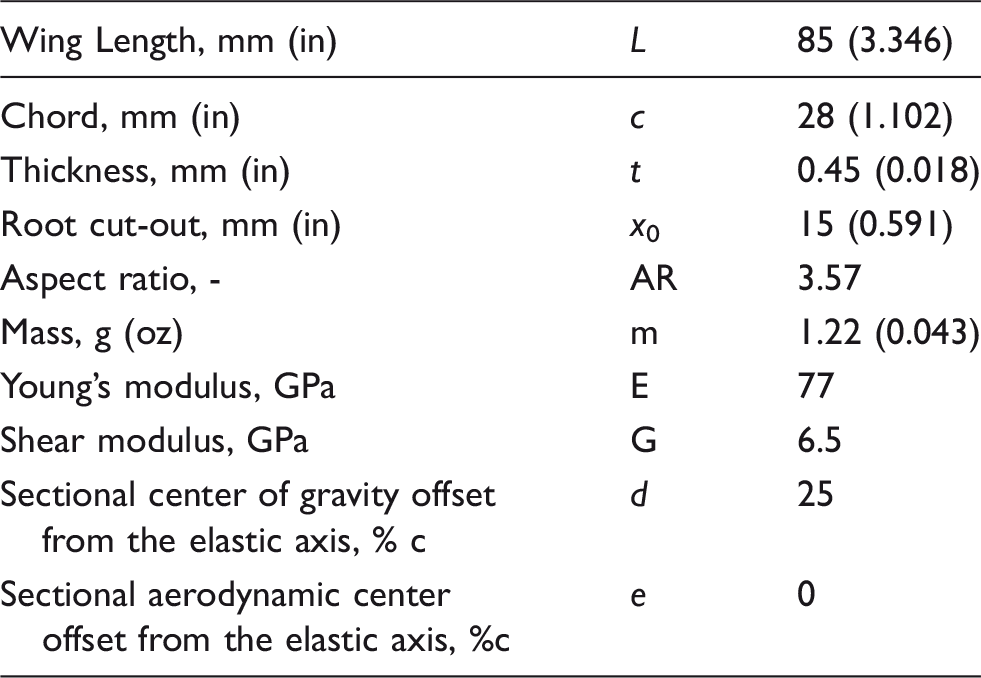
Figure 10 shows bending displacements for several points along the motion profile for the mid-chord clamped wing. The plot of tip displacement versus point on motion profile plot shows an out of phase sinusoidal profile when compared to the motion profile. The shifted phase of the displacements is due to aerodynamic loads which delay the zero-tip displacement point until points B or J.

Figure 10.

Mid-chord clamped wing.

The maximum tip displacements were found to occur at stroke reversals (points E, M) and the minimum tip displacements were found to be after the midstroke (points B, J). The maximum displacement points occur where both F _x and F _z are near their maximum. The maximum in F _z occurs at points F and N but these points are not where maximum deflection occurs because F _x rapidly drops off due to its higher frequency. The jump in F _z at points F and N seems to be a result of aerodynamic loading because it occurs after maximum acceleration on a sinusoidal motion profile.

Similar bending displacement measurements have been performed by Wu et al.²⁶ They tested Zimmerman planform wings composed of a carbon fiber skeleton and membrane skin. They found that maximum tip displacement occurred at approximately point F and N of the sinusoidal motion profile. The maximum displacement at stroke reversals found in this paper does not correlate with the findings by Wu et al. This is likely due to the much higher stiffness and mass of the wing used in this paper. The more flexible and lighter wing of Wu et al. is more affected by aerodynamic loads while the stiffer and heavier wing of this study is more affected by inertial loads. However, the vacuum condition tests performed by Wu et al. remove the effects of aerodynamics, so that deformations are due only to inertia. The vacuum tests showed maximum tip displacements at stroke reversal which matches what was found in this paper.

Error estimates for this study can be extracted directly from the displacement vectors calculated. The wing has been clamped with a rigid bar that is visible in the DIC images, and the displacement vectors of that bar should be zero. These have been zeroed in Figure 10 but are actually calculated to be close to zero in the post-processing. The maximum calculated bending displacement vector along the rigid clamp, which corresponds to the measurement error, ranged from 0.1 to 0.5 mm along the motion profile. This may be reduced if a smaller interrogation window is used.

Analytical results

The same geometry has been used to run numerical simulations as shown in Figure 1. However, the Reynolds number in experiment was still too high for DNS. In numerical simulation, the Reynolds number was reduced to Re = 700. POD modes were computed from the simulation data, and the most energetic eight modes were used to build a ROM with sufficient accuracy.

Figure 11 shows the first four POD modes, which capture 88% of the total energy. Large vortex structures are clearly captured in these modes. The ROM using the first eight mode captures 96.4% of the total energy. The phase portrait shows that the first and second modes have the fundamental frequency f, while the third and fourth modes have the frequency 2f (Figure 12). With only eight modes, though the coefficients computed by ROM are slightly different from the coefficients from the direct projection of DNS to the same low-order space, the fundamental dynamics is well kept as it is shown in Figure 12(a) and (b). Figure 12(c) shows the percentage of energy accumulatively captured by different number of modes.

Figure 11.

The votex structures of the first 4 POD modes. (a) mode 1, (b) mode 2, (c) mode 3, (d) mode 4.

Figure 12.

Phase portrait of coefficients (left) a₁ and a₂ (middle) a₁ and a₃, and (right) the accumulated energy distribution among POD modes.

In Figure 13, with only eight modes, the ROM computed and reconstructed the vortex structure with reasonable similarity in comparison to the same reconstruction by the DNS and its low-dimensional projection onto the same eight modes (a.k.a. POD reconstruction). Consistent with the observation in phase portrait, the ROM reconstruction is slightly different but still keeps all the core features well.

Figure 13.

Comparison of snapshots (at the same time) of flow fields reconstructed from the DNS, the direct projection of DNS data on the first eight POD modes, and the computation of the 8-mode ROM: (a) DNS, (b) POD reconstruction, (c) ROM.

To benchmark with experimental measurements, despite different Reynolds numbers, the forces along all three directions were plotted in Figure 14 to compare the calculation from the DNS, the direct POD projection on the same eight modes, and the eight-mode ROM using modified POD-Galerkin projection. The overall forces are smaller, reasonably, in simulation at lower Reynolds number, but all basic features are closely represented. With the symmetry in upstroke and downstroke for x direction, the force along x direction shows the period with only half of one flapping cycle in both experiment and computation; in y direction, the force is much smaller as expected and still shows some degree of accuracy even at this level with very small numbers; in z direction, the force response has the period the same as the flapping cycle, since the upstroke and downstroke have different contribution along it. Most important, within the computational results, the POD projection captures the main features from the DNS, and the ROM captures the main features with less but reasonable accuracy.

Figure 14.

Forces along three directions to compare the results from DNS (), direct projection in POD (), and ROM (): (a) F_x, (b) F_y, (c) F_z.

Conclusion

The objective of this study was to develop the methodology necessary for the reduced-order modeling of the loads and deformations of a flapping wing. An experimental setup capable of imparting an arbitrary flapping motion and measuring loads and deformations of a flapping wing was developed. Tests were performed on a uniformly stiff rectangular plate flapping in a 15 Hz, 40° stroke amplitude sinusoidal motion. A POD-Galerkin projection applied on a modified Navier–Stokes equation is able to give satisfactory accuracy in its comparison to the DNS, and both the numerical simulation and the ROM show the same dynamic features as those in the experiment at higher Reynolds number.

The pattern of maximum tip displacement at stroke reversal matches the pattern found in inertially dominated flapping wing deformation experiments performed in previous literature. The loading and displacement data can be correlated at specified points along the motion profile through the use of the encoder. The loading and displacements were larger for the quarter-chord clamped wing, and the surface plots showed an expected visible twisting. These experimental results for a simple rectangular plate will serve as a necessary validation step for future analytical ROMs.

While the current experimental setup does not capture the more complex kinematics and multi-wing aerodynamic interactions of biological flyers, the setup does provide a starting point from which a simple ROM may be developed. In fact, the ROM, which uses a POD-Galerkin projection approached tailored for moving boundaries and is based on numerical simulation data, shows satisfactory results in its comparison to the DNS data and its direct projection (i.e. POD and its time coefficients from POD analysis) in the same low-dimensional space. The above combined approach of experimental, simulation, and model reduction demonstrates a promising method for the study of flapping-wing MAVs and its optimization and on-board control. In future work, we will explore methods of measuring the wing deformation in real time and using the ROM to estimate the loads on the wing.

Footnotes

Declaration of conflicting interests

The author(s) declared no potential conflicts of interest with respect to the research, authorship, and/or publication of this article.

Funding

The author(s) disclosed receipt of the following financial support for the research, authorship, and/or publication of this article: This research was supported by U.S. Army Research Laboratory (ARL) through MAST CTA with Dr. Brett Piekarski and Dr. Christopher Kroninger as Technical Monitors.

References

Keennon M, Klingebiel K and Won H. Development of the nano hummingbird: a tailless flapping wing micro air vehicle. In: 50th AIAA aerospace sciences meeting, Nashville, TN, AIAA paper 2012-588, 9–12 January 2012.

de Croon

GCHE

de Clerq

KME

Ruijsink

et al.

Design, aerodynamics, and vision-based control of the delfly. Int J Micro Air Vehicles 2009; 1: 71–97.

Buchholz

JHJ

Smits

. On the evolution of the wake structure produced by a low-aspect-ratio pitching panel. J Fluid Mech 2006; 546: 433.

Dong

Mittal

Najjar

. Wake topology and hydrodynamic performance of low aspect-ratio flapping foils. J Fluid Mech 2006; 566: 309–343.

Dong

. Three-dimensional wake topology and propulsive performance of low-aspect-ratio pitching-rolling plates. Phys Fluids 2016; 28: 071901.

Koehler

Liang

Gaston

et al.

3d reconstruction and analysis of wing deformation in free-flying dragonflies. J Exp Biol 2012; 215: 3018.

Young

Walker

Bomphrey

et al.

Details of insect wing design and deformation enhance aerodynamic function and flight efficiency. Science 2009; 325: 1549.

Wei

Yang

et al.

An embedded boundary approach for the simulation of a flexible flapping wing at different density ratio. Eur J Mech 2016; 55: 146–156.

Zhao

Huang

Deng

et al.

Aerodynamic effects of flexbility in flapping wings. J R Soc Interf 2010; 7: 485.

10.

Dong

Liu

. Effects of a dynamic trailing-edge flap on the aerodynamic performance and flow structures in hovering flight. J Fluids Struct 2015; 58: 49.

11.

Wei

et al.

Adjoint-based optimization of flapping plates hinged with a trailing-edge flap. Theor Appl Mech Lett 2015; 5: 1–4.

12.

Wei

. Using adjoint-based optimization to study kinematics and deformation of flapping wings. J Fluid Mech 2016; 799: 56–99.

13.

Shoele

Zhu

. Performance of a wing with nonuniform flexibility in hovering flight. Phys Fluids 2013; 25: 041901.

14.

DeLaurier

. The development of an efficient ornithopter wing. Aeronaut J 1993; 97: 153–153.

15.

Larijani

DeLaurier

. A nonlinear aeroelastic model for the study of flapping wing flight. Prog Astronaut Aeronaut 2001; 195: 399–428.

16.

Singh

Chopra

. Insect-based hover-capable flapping wings for micro air vehicles: experiments and analysis. AIAA J 2008; 46: 2115–2135.

17.

Orlowski

Girard

. Modeling and simulation of nonlinear dynamics of flapping wing micro air vehicles. AIAA J 2011; 49: 969–981.

18.

Grauer

Hubbard

. Multibody model of an ornithopter. J Guidance Control Dyn 2009; 32: 1675–1679.

19.

DeLaurier

. An aerodynamic model For flapping-wing flight. Aeronaut J 1993; 97: 125–130.

20.

Vest

Katz

. Unsteady aerodynamic model of flapping wings. AIAA J 1996; 34: 1435–1440.

21.

Fritz

Long

. Object-oriented unsteady vortex lattice method for flapping flight. J Aircraft 2004; 41: 1275–1290.

22.

Roget

Sitaraman

Harmon

et al.

Computational study of flexible wing ornithopter flight. J Aircraft 2009; 46: 2016–2031.

23.

Faruque

Humbert

. Dipteran insect flightdynamics. part 1 longitudinal motion about hover. J Theor Biol 2010; 264: 538–552.

24.

Grauer

Ulrich

Hubbard

et al.

Testing and system identification of an ornithopter in longitudinal flight. JAircraft 2011; 48: 660–667.

25.

Willmott

Ellington

. The mechanics of flight in the hawkmoth manduca sexta. J Exp Biol 1997; 200: 2723–2745.

26.

Ifju

Stanford

. Flapping wing structural deformation and thrust correlation study with flexible membrane wings. AIAA J 2010; 48: 2111–2122.

27.

Sicard

Sirohi

. Measurement of the deformation of an extremely flexible rotor blade using digital image correlation. Measure Sci Technol 2013; 24: 065203.

28.

LaVision. StrainMaster DaVis 8.1., Germany: LaVision, 2012.

29.

Holmes

Lumley

Berkooz

. Turbulence, coherent structures, dynamical systems and symmetry, Cambridge: Cambridge University Press, 1996.

30.

Noack

Afanasiev

Morzynski

et al.

A hierarchy of low-dimensional models for the transient and post-transient cylinder wake. J Fluid Mech 2003; 497: 335–363.

31.

Wei

Rowley

. Low-dimensional models of a temporally evolving free shear layer. J Fluid Mech 2009; 618: 113–134.

32.

Wei

Qawasmeh

Barone

et al.

Low-dimensional model of spatial shear layers. Phys Fluids 2012; 24: 014108.

33.

Qawasmeh

Wei

. Low-dimensional models for compressible temporally developing shear layers. J Fluid Mech 2013; 731: 364–393.

34.

Sirovich

. Chaotic dynamics of coherent structures. Parts I–III. Quarter Appl Math 1987; XLV: 561–582.

35.

Zhao

Freund

Moser

. A fixed-mesh method for incompressible flow-structure systems with finite solid deformations. J Comp Phys 2008; 227: 3114–3140.

36.

Yang T and Wei M. A fully-coupled approach to simulate three-dimensional flexible flapping wings. In: 51st AIAA aerospace sciences meeting, Grapevine, TX, AIAA paper 2013-0864, 7–10 January 2013.

37.

Yang

Wei

Zhao

. Numerical study of flexible flapping wing propulsion. AIAA J 2010; 48: 2909–2915.

38.

Xu M, Wei M, Yang T et al. Nonlinear structural response in flexible flapping wings with different density ratio. In: 49th AIAA aerospace sciences meeting, Orlando, FL, AIAA paper 2011-376, 4–7 January 2011.

39.

Wei

Yang

. A global approach for reduced-order models of flapping flexible wings. In: 5th AIAA flow control conference. AIAA paper 2010-5085, Chicago, IL, 28 June–1 July 2010.

40.

Gao H and Wei M. Global model reduction for flows with moving boundary. In: 52nd aerospace sciences meeting, National Harbor, MD, AIAA paper 2014-0222, 13–17 January 2014.

Reduced-order methodology for prediction of loads generated by a flexible flapping wing

Abstract

Keywords

Introduction

Experimental setup and methodology

Wing properties

Flapping wing mechanism

Wing loads measurement

Deformation measurement

Experimental procedure

Analytical methods

Results and discussion

Experimental results

Analytical results

Conclusion

Footnotes

Declaration of conflicting interests

Funding

References