Sage Journals: Discover world-class research

Abstract

A method for the solution of the three-dimensional structural dynamics equations with large strains using a finite volume technique is presented. The proposed solution procedure is second order accurate in space and employs a second-order accurate dual time-stepping scheme. The momentum conservation equations are written in terms of the Piola-Kirchhoff stresses. The stress tensor is related to the Lagrangian strain tensor through the St. Venant-Kirchhoff constitutive relationship. The structural solver presented is verified through two test cases. The first test case is a three-dimensional cantilever beam subject to a gravitational load that is verified using theory and two-dimensional simulations reported in literature. The second test case is a three-dimensional highly deformable cantilever plate subject to a gravitational load. The results of this case are verified through a comparison with the modal response calculated by commercially available software. The focus of the current effort is the development and verification of the structural dynamics portion of a future fully coupled monolithic fluid-thermal-structure interaction code package.

Keywords

Structural dynamics finite volume method computational mechanics numerical methods

Introduction

During the design and analysis cycle of an aerodynamic system, engineers must develop an adequate understanding of the aeroelastic response of the body to properly estimate the fatigue life of the system components. This involves performing analyses over an array of aerodynamic conditions that encompass all likely aerodynamic disturbances to obtain a measure of the structural response. This process can be described as a fluid-structure interaction (FSI) analysis. In generic FSI problems, any change in the fluid domain will effect the response of the structural domain and vice versa.

There are two key considerations an analyst must make when developing an FSI simulation procedure. First, the extent of the coupling between the fluid and solid continuums. This will determine how frequently the fluid and the structural domains will exchange boundary condition information. Second, the selection of which numerical methods will be used to solve the fluid and solid governing equations (e.g. finite volume method). This will dictate if the FSI procedure will be monolithic or non-monolithic.

In non-monolithic approaches, the fluid and solid domain governing equations are solved using different numerical schemes. Doi and Alanso¹ used a finite volume fluid dynamics code with a commercial finite element structural solver to create a fully coupled non-monolithic FSI solver. However, it is more common to model the fluid physics with finite volumes and utilize the modal dynamic equations to simulate the structural response. Examples of this type of approach can be found in Liu et. al.,² Im et al.,³ Patel and Zha,⁴ and Sadeghi and Liu.⁵ This approach solves the structural equations in the frequency domain, which allows for larger solid domain time steps, thereby reducing the stiffness of the FSI method. However, high frequency behavior, modal coupling, and other non-linear behavior may go unnoticed by the structural solver.

Monolithic procedures use the same numerical method to solve the governing equations of fluid and solid continuums. These procedures must overcome two fundamental challenges: first, the fluid and solid governing equations are derived in the Eulerian and Lagrangian reference frames respectively. As a consequence, an Arbitrary Lagrangian Eulerian (ALE) method must be implemented to solve the governing equations of the two continuums simultaneously. Second, the maximum stable time step in the solid domain is typically much smaller than the maximum allowable fluid time step. This challenge is more difficult to overcome and generally causes monolithic FSI approaches to be numerically stiffer than non-monolithic approaches.⁶ Examples of monolithic approaches include Zorn and Davis,⁷ who used the finite volume method, and Gottfried and Fleeter,⁸ Turek and Hron,⁹ and Teixeira and Awurch,¹⁰ who used the finite element method.

In the current work, a general solution procedure of the three-dimensional structural dynamic equations using a finite volume formulation is presented. This structural dynamics solver is currently being integrated with an in-house finite volume fluid-thermal solver to create a monolithic fluid-thermal structural interaction (FTSI) solver.

The structural dynamics solution technique descried here expands upon the two-dimensional structural dynamics solver presented by Zorn and Davis.⁷ The governing equations for the solid continuum are solved using a Lax-Wendroff control volume technique with Ni’s¹¹ distribution algorithm and Jameson’s¹² point implicit dual time-stepping scheme, resulting in a simulation approach that is second-order accurate in space and time. With this approach, the equations are marched implicitly in time with a Newton-like inner iteration for each global time step. The momentum conservation equations are written in terms of the Piola-Kirchhoff stress and the displacement velocity components. The stress tensor is related to the Lagrangian strain and displacement tensors using the St. Venant-Kirchhoff constitutive relationship. The Piola-Kirchhoff stress is conceptually similar to engineering stress, as the reference condition is the undeformed solid geometry, rather than the instantaneous solid geometry as the more familiar Cauchy stress. This formulation allows for the integration of the structural equations using the undeformed configuration. This formulation is more computationally efficient because the cell face areas and cell volumes do not need to be recalculated at every local time step as they would for a Cauchy stress based approach.

Structural dynamics solution procedure

The solid domain is descritized into point-matched multi-block structured hexahedral finite volume grids. Two domains are defined for each solid cell, an instantaneous domain, denoted by $x_{i}$ , and a referential domain, denoted by $X_{j}$ . The instantaneous domain reflects the actual shape and deformations applied to the current grid cell, whereas the referential domain is an undeformed cell used for integration purposes. These two domains are related to each other by the configuration array, $F_{i j}$ , which is essentially a Jacobian array that allows coordinate mapping between the two domains, as shown in equation (1). The configuration array is related to the displacement gradient by equation (2), where $I$ is the identity matrix.

Configuration array

F_{i j} = \frac{\partial x_{i}}{\partial X_{j}}

(1)

Displacement gradient configuration array relationship

\frac{\partial D_{i}}{\partial X_{j}} = F_{i j} - I_{i j}

(2)

The desired quantities in the solid blocks are the displacement,

D_{i}

, and velocity,

v_{i}

, of the nodes. The nodal displacement can be determined from the integration of the strain field,

E_{i j}

, as denoted in equation (3). This definition of the strain field allows for large deformations and thermal strain; where

β_{s}

is the coefficient of thermal expansion,

T_{S}

is the temperature of the solid and

T_{R}

is the prescribed reference temperature which is an input value. Two stress tensors are utilized to describe the physical state of the solid material, the

1 st

and

2 nd

Piola-Kirchhoff stresses. The

2 nd

Piola-Kirchhoff stress,

S_{i j}

, is related to the strain through the St. Venant-Kirchhoff constitutive relationship, as shown in equation (6). The

1 st

and the

2 nd

Piola-Kirchhoff stresses are related using the configuration array as shown in equation (7). The

1 st

Piola-Kirchhoff stress,

P_{i j}

, allows a direct mapping of forces to the referential configuration. This connection is exploited to relate the solid momentum equation with the stress field as described in equation (9). The Lamé parameters

λ

and

μ

are related to Young’s modulus, E, and Poisson’s Ratio,

ν

, as denoted in equations (4) and (5). Finally, the

2 nd

Piola-Kirchhoff stress and the Cauchy stress,

σ_{i j}

, are related by equation (8). The temperature field in the solid domain is modeled with the heat conduction equation, as shown in equation (10). Equations (9) and (10) are the main time-dependent governing equations solved with the point-implicit dual time step, finite volume technique.

Strain/displacement relation

E_{i j} = \frac{1}{2} (\frac{\partial D_{i}}{\partial X_{j}} + \frac{\partial D_{j}}{\partial X_{i}} + \frac{\partial D_{k} \partial D_{k}}{\partial X_{i} \partial X_{j}}) + β_{x} (T_{S} - T_{R})

(3)

First Lamè parameter

λ = \frac{ν E}{(1 + ν) (1 - 2 ν)}

(4)

Second Lamè parameter

μ = \frac{E}{2 (1 + ν)}

(5)

St. Venant-Kirchhoff constitutive relationship

S_{i j} = λ δ_{i j} E_{k k} + 2 μ E_{i j}

(6)

First and Second Piola-Kirchhoff stress relation

P_{i k} = F_{i j} S_{j k}

(7)

Cauchy stress and first Piola-Kirchhoff stress relation

σ_{i k} = \frac{1}{| F |} P_{i j} F_{k j}

(8)

Solid momentum equation

ρ_{s} \frac{\partial v_{i}}{\partial t} - \frac{\partial P_{i j}}{\partial X_{j}} = f_{i}

(9)

Heat conduction equation

ρ_{s} C_{p s} \frac{\partial T}{\partial t} = k_{s} \frac{\partial^{2} T_{s}}{\partial X_{j}^{2}}

(10)

Time marching

The point-implicit dual time step method formulated by Jameson¹² is used in the current study, described in equation (11); where $n$ is the global time step and $m$ is the inner iteration index, $v$ is the nodal velocity, $F (v^{m})$ represents the $\frac{1}{ρ_{s}} (f_{i} + \frac{\partial P_{i j}}{\partial X_{j}})$ terms of the solid momentum equation (9) for the current inner iteration. This method is marched implicitly by a specified value of $Δ t_{G}$ , but the equations are solved at each global time step iteratively using a local time step of $Δ t_{L}$ until the residual drops below a tolerance. The local time step, $Δ t_{L}$ is determined from equation (12). Each grid cell has an independent local time step size, $Δ t_{L}$ , based on a specified Courant-Friedrichs-Lewy (CFL) number, the geometry of the cell, and material properties assigned to the cell, as described in equation (12); where $V_{o l}$ is the cell volume, $A_{i s}$ , $A_{j s}$ , $A_{k s}$ are one-half of the root-sum-square of the cell face areas, and $i, j, k$ subscripts refer to the three-dimensional grid directions. For the current study, the inner iteration convergence tolerance was on the order of $10^{- 5}$ , this typically took about 100 inner iterations, and the $C F L$ was set to 0.9.

Dual time stepping method¹²

\begin{aligned} \begin{matrix} v^{m + 1} = F (v^{m}) Δ t_{L} \\ + \frac{- 3 v^{m} + 4 v^{n} - v^{n - 1}}{2 Δ t_{G}} Δ t_{L} + v^{m} \end{matrix} \end{aligned}

(11)

Minimum local time step calculation

\min (Δ t_{L}) = \frac{C F L V_{o l}}{2 \sqrt{\frac{E}{ρ} (A_{i s} + A_{j s} + A_{k s})}}

(12)

The dual time-stepping method presented in equation (11) is chosen for two reasons. First, the goal of the presented structural solver is to be integrated into an existing fluid-thermal interaction finite volume code that uses this dual time-stepping method. Second, this point-implicit method allows for the simulation to be executed with a larger time step, that is two to four orders in magnitude larger than the explicit time step given by equation (12). As will demonstrated below, the dual time stepping method can typically reduce simulation time by

25 %

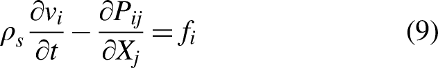
The solid momentum equation (9) is a second-order partial differential in terms of displacement. Therefore, a second time integration is necessary to determine the nodal displacement. This is completed using equation (13), which is a second-order accurate backward difference equation; where $m$ and $n$ are the inner and outer iteration indices respectfully, $D$ is the nodal displacement, $Δ t_{G}$ is the global time step, and $v$ is the nodal velocity.

Displacement time integration⁷

D^{m + 1} = \frac{2 v^{m + 1} Δ t_{G} + 4 D^{n} - D^{n - 1}}{3}

(13)

Hourglass stiffening

Due to the second-order accurate discretization of the solid domain using finite volumes, a numerical issue arises called hourglassing.⁸ For hexahedral cells, there are eight deformation modes; four of the eight deformation modes pertain to rigid body motion, expansion/contraction, and two shear modes that are all permissible modes of deformation. However, four hourglass modes exist which represent unconstrained motion that can lead to the destruction (decoupling) of the solution. Each hourglass mode has a corresponding basis vector denoted by $Γ_{l k}$ , listed in Table 1. Hourglass modes are represented pictorially in Figure 1. The hourglassing phenomena is similar to the odd–even decoupling that can occur in second-order accurate central-difference, finite-difference, or finite volume solvers. To prevent the destruction of the solution, a fictitious force is introduced at each solid node to discourage the unconstrained movement. The hourglass force is described by equation (15); where $F_{i l}^{h g}$ is the artificial smoothing force, $h_{i j}$ is a measure of how much a node is allowed to move in an unconstrained manner, and $Q_{h g}$ is the hourglass coefficient. The hourglass force is ultimately added to the right hand side of equation (9) as an additional nodal force. Note that the current study calculates $h_{i j}$ based on nodal displacement, rather than nodal velocity as proposed by Gottfried and Fleeter,⁸ per the findings of Zorn and Davis.⁷ Gottfried and Fleeter⁸ recommended $Q_{h g}$ to be between $0.05$ and $0.15$ . In the current study, all simulations use an hourglass coefficient of $0.05$ .

Figure 1.

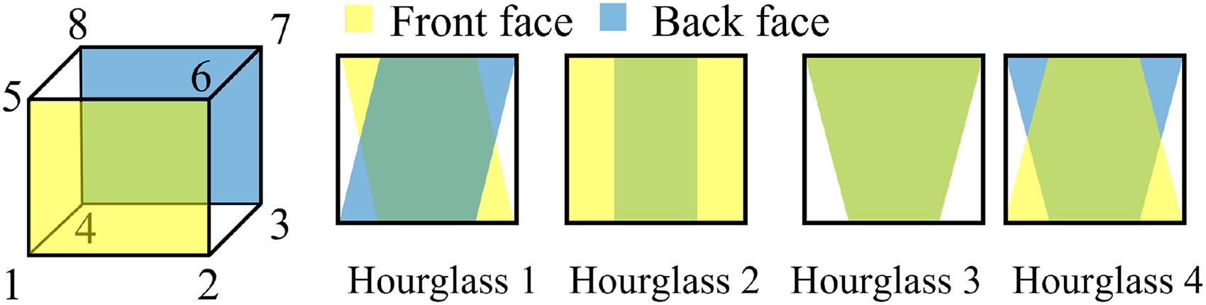
Description of hourglass deformation modes.

Table 1.

Hourglass modes notation for equations (14) and (15).⁸

	Local node number
Deformation mode	1	2	3	4	5	6	7	8
Hourglass 1 $Γ_{l 1}$	$-$ 1	$-$ 1	1	1	1	1	$-$ 1	$-$ 1
Hourglass 2 $Γ_{l 2}$	$-$ 1	1	1	$-$ 1	1	$-$ 1	$-$ 1	1
Hourglass 3 $Γ_{l 3}$	1	$-$ 1	1	$-$ 1	1	$-$ 1	1	$-$ 1
Hourglass 4 $Γ_{l 4}$	1	$-$ 1	1	$-$ 1	$-$ 1	1	$-$ 1	1

Hourglass magnitude⁷

h_{l k} = \frac{D_{i l} Γ_{l k}}{Δ t_{L}}

(14)

Hourglass force⁸

F_{i l}^{h g} = - ρ V^{2 / 3} (0.25 Q_{h g} A + 25 Q_{h g}^{2} | h_{i k} |) h_{i k} Γ_{l k}

(15)

Parallel processing

The structural solver presented in this work has been developed to support massively parallel processing. The solid domain may be decomposed into separate point-matched, hexahedral computational blocks to improve the speed of computation. Computational blocks can be assigned to any number of processors provided that the number of processors is less than or equal to the number of blocks. The nodal displacement, velocity, and forces are message passed to adjacent inter-block boundaries at every inner iteration using the message passing interface (MPI). The message passing process ensures that the nodal displacement, velocity, and forces are consistent and continuous at all inter-block boundaries. All messages are sent with non-blocking communication. Figure 2 is an example of a grid decomposed into four computational blocks.

Figure 2.

Computational grid for the beam case decomposed into four computational blocks.

The computational grid shown in Figure 2 is created by a utility developed for this effort which generates multi-block grid files. The computational grid is read by the in-house solver and load balanced among available processors. If there are more computational blocks in the grid file than available processors, then multiple computational blocks will exist on some processors and a load balancing of the processors is conducted. The load balancing approach aims to load each processor with computational blocks (with associated weights) to achieve a uniform weight distribution across all processors. A computational block’s weight is determined by the number of points in the block and the number of points along the faces of the block.

All simulations presented in this work were conducted on the HPC1 cluster located at the University of California, Davis. The HPC1 cluster consists of 60 compute nodes, each with 2 Intel E5-2630 v3 2.4 GHz CPUs and eight cores with hyper-threading. An Intel QDR Infiniband network adaptor is used for high speed communications between nodes. For the present study, a maximum of seven cores were used on one node.

Solution process

The structural solver discussed in this work may be implemented following the 13 steps listed below:

Calculate and store undeformed cell face areas and volumes.

Begin outer iterations.

Begin inner iterations.

Determine local time step, equation (12).

Calculate hourglass stiffening artificial force, equation (15).⁸

Calculate cell centered displacement gradient and strains, equation (3).

Use St. Venant-Kirchhoff constitutive relationship to find second Piola-Kirchhoff Stress, equation (6).

Use configuration array to calculate $1 st$ Piola-Kirchhoff stress, equation (7).

Distribute changes in solid momentum to cell nodes using Ni’s¹¹ distribution algorithm.

Calculate nodal velocities and displacements using equations (11) and (13).

Ensure that nodes at inter-block boundaries have the same displacement, velocity, and forces.

Update computational grid.

Check inner-iteration convergence tolerance, if met proceed to next global time step/outer iteration. If not, repeat steps 4 to 12.

Results

Two test cases have been chosen to demonstrate the capability of the proposed structural solver. The first is a flexible cantilever beam subject to a gravitational load. This three-dimensional test case is inspired by a two-dimensional test case proposed by Turek and Hron,¹⁰ also simulated by Zorn and Davis.⁷ The purpose of the first test case is to verify the implementation of the three-dimensional structural solver against literature and theoretical results. The second test case is a highly flexible square cantilever plate subject to a gravitational load. The purpose of this test case is to verify the stability and accuracy of the structural solver with a test case that has arbitrarily large strains. This test case is verified with commercially available software.

Cantilever beam

The simulation parameters for a cantilever beam vibrating due to a gravitational load can be found in Table 2. The computational grid used for this study is shown in Figure 3. The left side of the domain is fixed, while all other faces have a reflective boundary condition applied where time-rate changes in nodal acceleration are doubled to prevent span wise variations in nodal displacement and velocity. This boundary condition application enables the comparison of the three-dimensional solver with the two-dimensional results.^7,9 Zorn and Davis⁷ solved the two-dimensional structural momentum equations using a control-volume approach that is described in this work. Turek and Hron⁹ employed the finite element method to solve the two-dimensional structural momentum equations.

Figure 3.

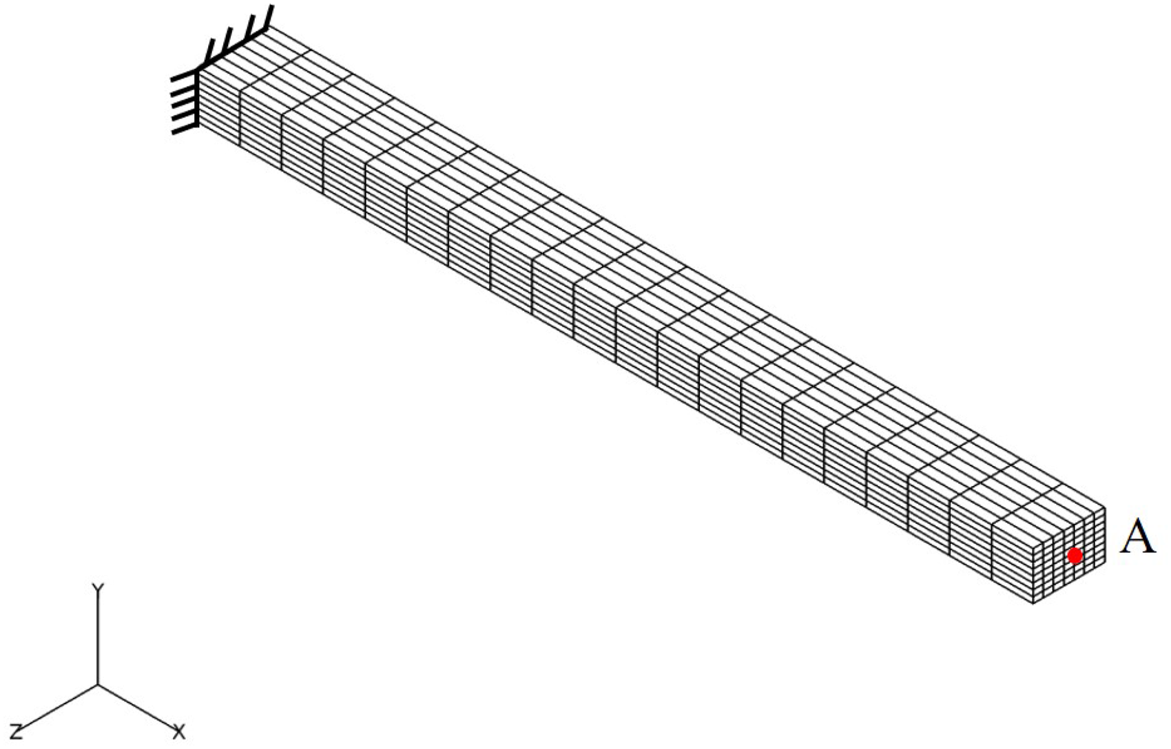
Computational grid for the beam case; point A is used to track the displacement and velocity of the beam throughout the simulation.

Figure 4.

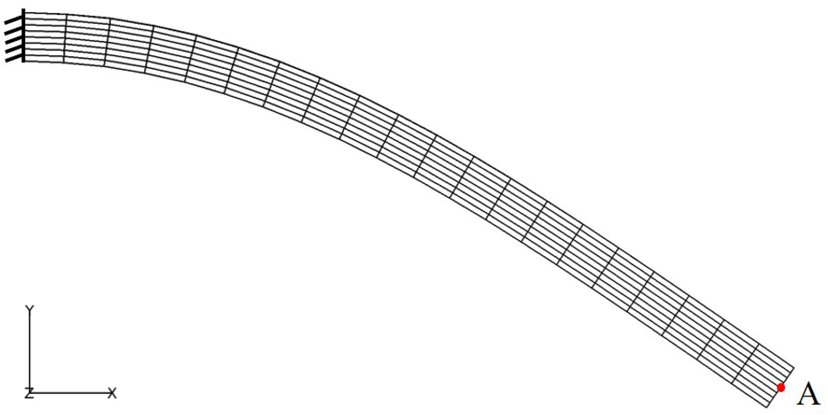
Beam grid at maximum deflection.

Table 2.

Simulation parameters for cantilever beam case.

Physical property	Value
Density ( $kg / m^{3}$ )	1000
Young’s modulus (MPa)	1.4
Poisson ratio	0.4
Gravitational acceleration ( $m / s^{2}$ )	2.0
Beam length (m)	0.35
Beam height (m)	0.02
Beam width (m)	0.03

The displacement history of point A in Figure 3 is tracked throughout the simulation. The beam grid shown in Figure 3 has 1512 grid points and has been decomposed into four computational blocks. The displacement time histories of the current study, using a time step of $5 \times 10^{- 6}$ s, is compared with the time histories reported by Zorn and Davis⁷ and Turek and Hron⁹ in Figure 5. The maximum X and Y deformation of point A is $0.0381 m$ and $0.142 m$ , respectively. Zorn and Davis⁷ reported the maximum displacement of $0.022 m$ and $0.120 m$ , while Turek and Hron $^{9}$ reported $0.029 m$ and $0.130 m$ . The discrepancy between maximum reported the displacements by Zorn and Davis,⁷ Turek and Hron,⁹ and the current study is caused by the three-dimensional effects of the strain equations.

Figure 5.

Three-dimensional (3D) cantilever beam case displacement time histories compared with two-dimensional (2D) studies.^7,9

For further solution verification, displacement time history of point A is compared with the theoretical natural frequency of a cantilever beam subject to a body force, described in equation (16)¹³; where $f_{n}$ is the natural frequency of the current mode, $K_{n}$ is the vibration constant, where n refers to the mode of vibration ( $K_{1} = 3.52$ , $K_{2} = 22.0$ , $K_{3} = 61.7$ ), $I$ is the area moment of inertia and $w$ is the force per unit length applied to the beam. The first three theoretical modal frequencies are 0.988, 6.173, and 17.31 Hz. Equation (16) is useful to compare the two-dimensional and three-dimensional simulations because the theoretical beam frequency is independent of the depth of the beam, as long as the beam aspect ratio is 8 or greater.¹³ The modal frequencies of the current simulation are determined by conducting a discrete Fourier transform (DFT) on the $Y$ displacement history of the tracked point. The results of this operation are compared with theory and results reported by Zorn and Davis⁷ and Turek and Hron⁹ are summarized in Table 3. The method for solving the structural equations presented in this work predict the first three modes of vibration more accurately than the structural solvers presented Zorn and Davis⁷ and Turek and Hron.⁹ Theoretical natural frequency for a cantilever beam subject to uniform loading¹³:

f_{n} = \frac{K_{n}}{2 π} \sqrt{\frac{E I g}{w l^{4}}}

(16)

Table 3.

Comparison of theoretical modal beam frequencies and those predicted by current study, Zorn and Davis⁷ and Turek and Hron.⁹

	Theory	Current study		Zorn and Davis $^{7}$		Turek and Hron $^{9}$
Mode	Frequency (Hz)	Frequency (Hz)	$%$ Error	Frequency (Hz)	$%$ Error	Frequency (Hz)	$%$ Error
1	0.989	1.00	1.25	1.05	6.31	1.10	11.37
2	6.17	6.10	1.18	No data		No data
3	17.31	16.50	4.69	No data		No data

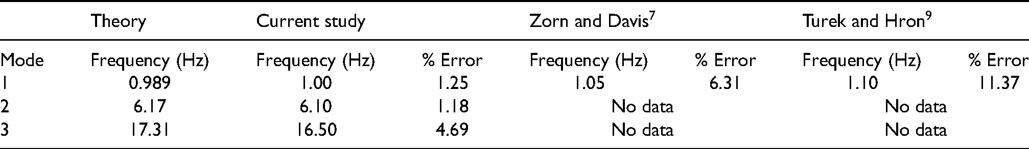
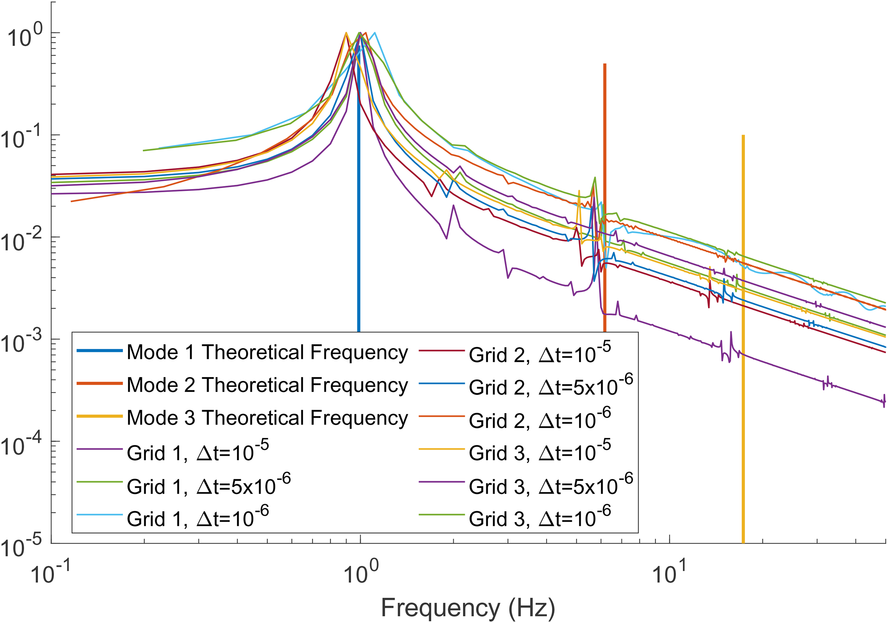
A grid and temporal convergence study has been conducted to establish solution independence. Three grids have been created for this study; grid 1 has 1512 grid points-shown in Figure 3—grids 2 and 3 have 2376 and 2772 grid points, respectively. Each grid has been run with three global time steps, $10^{- 5}$ , $5 \times 10^{- 6}$ , and $10^{- 6}$ s. A DFT has been conducted on the $Y$ displacement history data on all of the aforementioned cases and the results are shown in Figure 6. A grid and time step is considered to be accurate if the calculated modal frequency for the first mode is within $\pm 5 %$ of the theoretical value. All grids meet this criteria for time steps $5 \times 10^{- 6}$ and $10^{- 6}$ s. However, only grid 1 meets this criteria for the $10^{- 5}$ s time step size.

Figure 6.

Discrete Fourier transform (DFT) of beam tip Y displacement data.

Results of the grid and temporal convergence study are also used to verify that the presented solution method is at least second order accurate. The order of accuracy of a numerical scheme¹⁴ can be determined though the use of equation (17); where $E$ is the percent error, $C$ is some constant, and $P$ is the formal spatial order of accuracy of a numerical scheme, and $Δ x$ is the cell volume. The constant C is only important in determining the absolute level of errors in the order of accuracy. By taking the natural logarithm of equation (17), the formal order of accuracy can be determined from a series of solutions with increasingly refined grids using equation (18), where P is the slope of $l n (E)$ versus $l n (Δ x)$ .

Computational error calculation¹⁴

E = C Δ x^{P}

(17)

Modified computational error¹⁴

l n (E) = P l n (Δ x) + l n (C)

(18)

The first mode frequencies predicted by each grid with time step

5 \times 10^{- 6}

s can be used to determine the computational error. The order of accuracy of this method is found by plotting

l n (E)

versus

l n (Δ x)

using the data from Table 4 and calculating the line of best fit through the data points. With the limited number of grid refinements used in the current investigation, the spatial order of accuracy of this method is found to be

2.816

Table 4.

Global time step $5 \times 10^{- 6}$ s simulation results; used to determine the presented method’s order of accuracy.

Grid	Cell volume ( $m^{3}$ )	$1 st$ mode Freq. (Hz)	$%$ Error
1	$1.906 \times 10^{- 7}$	0.9995	1.197
2	$1.158 \times 10^{- 7}$	0.998	1.045
3	$9.880 \times 10^{- 8}$	0.997	0.944

To demonstrate benefits of developing a massively parallel structural solver algorithm, a computational speed test has been conducted. The four block computational grid shown Figure 2 is simulated for 1000 iterations with four blocks on one processor (serial), and with one block per processor (parallel). The serial case and parallel case had average run times of 352 and 160 s, respectively. Parallel efficiency of the algorithm can be calculated using $η = \frac{t_{s e r i a l}}{n * t_{p a r a l l e l}}$ ; where $n$ is the number of processors. The resulting parallel efficiency for this case is 55%.

To demonstrate the simulation speed increase using the dual time-stepping method presented in equation (11), consider grid 1 shown in Figure 3. The minimum time step for this grid is $8.05 \times 10^{- 8}$ s, using equation (12). While an accurate solution has been obtained for this gird with a global time step of $10^{- 5}$ s with 100 inner iterations. In this instance, the dual time stepping method can deliver speed increases around 24%.

Highly flexible cantilever plate

To further demonstrate the capabilities of this structural solver, a three-dimensional highly flexible plate case is considered. The goal of this case is to demonstrate the versatility of the structural solver, by capturing multiple modes of a highly flexible plate in free vibration. Simulation parameters are identical to those used by the beam case, listed in Table 2, except the plate width is 0.35 m, and the plate thickness is 0.01 m. The plate is subject to a $2 {m / s}^{2}$ gravitational acceleration. A fixed boundary condition is applied to the left side of the domain and all other faces are free. The displacement of three points—A, B, and C in Figure 7—on the plate tip are tracked throughout the simulation. The plate grid has 3969 grid points, decomposed into a maximum of seven computational blocks. The plate experiences a maximum x and y displacement of 0.297 and 0.303 m, respectively. Figure 8 shows the plate grid 1 at the maximum deflection.

Figure 7.

Plate computational grid, 3969 grid points. Points A, B, and C are tracked throughout the simulation.

Figure 8.

Plate grid 1 at maximum deflection.

A time history plot for the plate grid with a global time step of $2.5 \times 10^{- 6}$ s is shown in Figure 9(a) and (d). Figure 9(b), (c), (e) and (f) shows the detail views of the maxima and minima of displacement history for the first deformation cycle to demonstrate how the displacement varies across the span of the plate.

Figure 9.

Plate simulation displacement history of points A, B, and C for grid 1 $Δ t = 2.5 \times 10^{- 6}$ s.

To verify the plate simulations, a modal model of the plate was created in the commercial code ANSYS DiscoveryAIM. To establish solution independence, two meshes were created using eight node hexahedral elements. The first mesh had 450 nodes, the second mesh had 1152 nodes. A fixed boundary condition was applied to the left face of the plate, all other faces are free. The first three modes calculated for each mesh are 0.526, 1.230, 3.179 Hz, and 0.525, 1.224, 3.15 Hz, respectively. The modal frequencies calculated by ANSYS on the second mesh have been used to verify the frequency response of the plate calculated by the current method. The frequency response of the plate simulation is determined by conducting a DFT on the displacement time history of point A. Table 5 compares the results of the plate simulation with 3969 grid points and a time step of $2.5 \times 10^{- 6}$ s with the 1152 node ANSYS mesh. There is very good agreement between ANSYS and the in-house code presented for the first two modes. The third mode predicted using the current method is 1.71 Hz and does not agree with ANSYS predictions.

Table 5.

Comparison plate modal frequencies predicted by current study and ANSYS-discovery AIM.

	ANSYS-DiscoveryAIM	Current study
Mode	Frequency (Hz)	Frequency (Hz)	$%$ difference
1	0.525	0.571	8.1
2	1.224	1.286	4.8

To establish solution independence a grid and temporal convergence study was conducted on the plate. The first plate grid was run at an additional global time step of $10^{- 6}$ s, and a second grid with 8624 points was created and run at both time steps. A DFT was then conducted on the displacement history of point A for each grid. All simulations were run for $7$ s of physical time, which allows the plate to complete three and a half deformation cycles. The results of this grid study are shown in Figure 10. The first mode frequencies predicted by both meshes and time steps are within $\pm 5 %$ of each other, and demonstrate good agreement with ANSYS frequency predictions satisfying the grid and temporal convergence requirements.

Figure 10.

Discrete Fourier transform (DFT) of plate Y displacement time histories of point A.

To demonstrate the benefits of massively parallel computing, a computational speed test for the cantilever plate case has also been conducted. Plate grid 1, shown in Figure 7, is decomposed into seven equally sized computational blocks. Then, a simulation is conducted for 1000 iterations serially (with seven blocks on one processor) and in parallel (with one block per processor). The serial case and parallel case had average run times of 1222 and 221 s, respectively. The resulting parallel efficiency is $79 %$ . This parallel efficiency value is $24 %$ larger than that reported in the beam case because the computational size (overall number of grid points as well as the ratio of block grid points to block face grid points) of the plate case lends itself to parallelism. The number of points per processor for the parallel beam case is 432, while the plate case has 567 points per processor.

Summary

A finite volume solution procedure for the structural dynamics equations that has been presented. A detailed methodology for the implementation of this structural solver has been given. Two test cases were presented for the verification of the proposed structural dynamics procedure. The first test case was a three-dimensional cantilever beam that was inspired by a two-dimensional test case proposed by Turek and Hron⁹ and repeated by Zorn and Davis.⁷ The proposed solver demonstrated excellent agreement with theoretical vibratory response of a cantilever beam and good agreement with literature.^7,9 The second test case was a highly flexible square cantilever plate subject to a gravitational load. The first two modal frequencies predicted by the presented structural solver show good agreement with the commercial code ANSYS-Discovery AIM. The structural solver presented in this work is currently being integrated into a finite volume fluid-thermal interaction code to develop a monolithic fully coupled fluid-thermal-structure interaction code package.

Footnotes

Acknowledgements

The authors would like to thank the managers at the Air Force Research Lab (AFRL) and Florida Turbine Technology (FTT) for their support. The authors would also like to thank the managers of Field View Inc., for providing an academic license to the FieldView Scientific Visualization system.

Declaration of conflicting interests

The authors declared no potential conflicts of interest with respect to the research, authorship, and/or the publication of this article.

Funding

The authors disclosed receipt of the following financial support for the research, authorship, and/or publication of this article. This effort was partially supported by the Air Force Research Laboratory (AFRL) under Florida Turbine Technologies (FTT) contract agreement FTT16-0403 SPO #201603132 with Dean Johnson and Ryan Brearly as the contract monitors as well as the University of California, Davis Graduate Studies.

ORCID iD

Joseph S Graff

References

Doi

Alonso

. Fluid/structure coupled aeroelastic computations for transonic flows in turbomachinery. In Volume 4: Turbo Expo, 2002, Parts A and B. Amsterdam, The Netherlands: ASMEDC. pp. 787–794.

Liu

Cai

Zhu

et al. Calculation of wing flutter by a coupled fluid-structure method. J Aircr 2001; 38(2): 334–342.

Chen

Zha

. Detached eddy simulation of transonic rotor stall flutter using a fully coupled fluid-structure interaction. In Volume 6: Structures and Dynamics, Parts A and B. Vancouver, British Columbia, Canada: ASMEDC. pp. 1217–1230.

Patel

Zha

. Improved delayed detached eddy simulation of AGARD wing flutter with fully coupled fluid-structure interaction. In AIAA Scitech 2021 Forum. American Institute of Aeronautics and Astronautics. pp. 1–16.

Sadeghi

Liu

. Coupled fluid-structure simulation for turbomachinery blade rows. In 43rd AIAA Aerospace Sciences Meeting and Exhibit. Reno, Nevada: American Institute of Aeronautics and Astronautics.

Hou

Wang

Layton

. Numerical methods for fluid-structure interaction—A review. Commun Comput Phys 2012; 12(2): 337–377.

Zorn

Davis

. Procedure for 2D fluid-structure interaction simulation. J Algorithm Comput Technol 2019; 13 1–12. DOI: 10.1177/1748302619861734

Gottfried

Fleeter

. Aerodynamic damping predictions in turbomachines using a coupled fluid-structure model. J Propul Power 2005; 21: 327–334.

Turek

Hron

. Proposal for a numerical benchmarking of fluid-structure interaction between an elastic object and laminar incompressible flow. Fluid-structure interaction modeling, simulation optimization. Berlin Heidelberg: Springer, Vol. 53, pp. 371–385.

10.

Teixeira

Awruch

. Numerical simulation of fluid–structure interaction using the finite element method. Comput Fluids 2005; 34(2): 249–273.

11.

. A multiple grid scheme for solving the euler equations. AIAA J 1982; 1565–1571.

12.

Jameson

. Time dependent calculations using multi-grid, with applications to unsteady flows past airfoils and wings. In: 10th Computational Fluid Dynamics Conference, 1991. American Institute of Aeronautics and Astronautics.

13.

Roark

Young

Budynas

. Roark’s formulas for stress and strain. 7th ed. New York: McGraw-Hill, 2002.

14.

Chetty