Sage Journals: Discover world-class research

Abstract

A numerical technique for the solution of the structural dynamics equations of motion is presented. The structural dynamics mass and momentum conservation equations are solved using a control volume technique which is second-order accurate in space along with a dual time-step scheme that is second order accurate in time. The momentum conservation equation is written in terms of the Piola–Kirchoff stresses and the displacement velocity components. The stress tensor is related to the Lagrangian strain and displacement tensors using the St. Venant–Kirchoff constitutive relationship. Source terms are included to account for surface pressure and body forces. Verification of the structural dynamics solution procedure is presented for a two-dimensional vibrating cantilever beam. In addition, the structural dynamics solution procedure has been implemented into a general purpose two dimensional conjugate heat transfer solution procedure that uses a similar dual time-step control volume technique to solve the fluid mass, energy, and Navier–Stokes equations as well as the structural energy heat conduction equation. The resulting overall solution procedure allows for solutions to fluid/structure, fluid/thermal, or fluid/thermal/structure interaction problems. Verification of the multidisciplinary procedure is performed using a cylinder with a flexible solid protruding downstream that mimics a cylinder-flag configuration. The approach is a proof of concept for compressible flow with continuum based solids. The methods are currently being extended to 3D flow fields and solids.

Keywords

Computational fluid dynamics finite volume method fluid–structure interaction numerical methods structural dynamics

Introduction

During the design cycle of aerodynamic configurations, engineers limit the possibility of structural fatigue through analysis of resonant modes at design and off-design conditions. In the past, this has involved performing analyses of an array of aerodynamic conditions that encompass all likely aerodynamic disturbance frequencies and phase of vibrations to obtain a measure of the structural damping response, known as the aerodynamic damping. Aerodynamic damping is a measure of the work done by the unsteady aerodynamic forces on the aerodynamic body. When the aerodynamic damping becomes negative and relatively large, the resulting aerodynamic body motion is unstable and steps are taken to change the design by increasing thickness or other geometric parameters and/or by altering the flow.

Analyses performed over the array of unsteady aerodynamic conditions to determine aerodynamic damping have traditionally involved first performing steady finite element analysis of the aerodynamic body to determine the resonant mode shapes and frequencies. Next, Navier–Stokes analyses of fixed, rigid geometry are performed at each aerodynamic condition to determine the mean flow field. After that, analyses of the unsteady (perturbation) flow are performed at each mean-flow aerodynamic condition corresponding to the possible forcing modes, frequencies, and vibration phases that could occur. Each analysis provides a prediction of the aerodynamic damping for those conditions. By performing these analyses in the frequency domain rather than in the time domain, each analysis can be performed fairly quickly similar to the steady mean flow analysis. The array of analyses can thus determine under what aerodynamic conditions and what areas of the aerodynamic body where resonant stress/fatigue might be possible through the prediction of the aerodynamic damping.

Many times the continuum of the structure is reduced to simple deformation elements, such as a combination of a torsion bar and a spring, for structure fluid interaction simulation. This is often done in 2D problems as the 3D physics of a continuum structural domain is difficult to reduce for many practical structure/fluid interaction problems. Nguyen et al.¹ provide an example of this method in which he reduces the wing of a commercial plane down to a spring and a torsion bar. Ou and Jameson perform 2D examples with a torsional spring on a pitching airfoil and with a cylinder attached to a spring.²

A common method of modeling structure/fluid interaction is the modal method. In standard mesh decomposition, the difference in stable time step for the structural domain, and the fluid domain is usually too large. In order to compensate for this, the structural domain is decomposed into dominant deformation modes to reduce the need for exceedingly small time steps in the structural domain. Many times the structural domain and the fluid domain are not marched at the same rate; the solid domain is marched at large implicit time steps while the fluid domain is marched at small explicit time steps. Harash et al. has performed examples of this method.^3,4 Quan et al. perform an example of the modal method using a delta wing.⁵ Liu et al. have also performed 3D fluid/structure interaction (FSI) examples using the modal method observing the airfoil shape, AGARD 445.6.⁶

In turbomachinery, a series of decoupled analysis are often performed. The physics of the structure is not modeled with the flow. Instead, the motion of the structural domain is prescribed in one of the dominant deformation modes, while the flow is modeled around the motion of the moving blade. The solution is obtained in the frequency domain for a faster analysis. From this analysis, aerodynamic damping is extracted. This method typically results in a series of simulations that utilize multiple blade deformation modes on multiple points of the performance curve of the compressor or turbine. The series of simulations is further increased by the observation of multiple blade rows because the series must account for multiple vibration modes for the various blade rows, as well as different phase angles for the different blade rows and passages. Examples can be seen in Hoyniak and Clark’s⁷ and Hall and Clark’s⁸ papers.

The structural dynamics solution approach used in this investigation consists of a time-marching, control volume scheme that solves the integral form of the mass and momentum conservation equations. A dual time-step algorithm is used to integrate the governing equations in time for both solid and fluid mechanics in a monolithic approach. The resulting numerical approach is second-order accurate in space and time that is tightly coupled between the solid and fluid domains. The structural dynamics momentum equation is written in terms of displacement velocity components and the first Piola–Kirchhoff stress tensor. Surface pressure and body forces are included as source terms. The stress tensor is related to the Lagrangian strain and displacement tensors using the St. Venant–Kirchhoff constitutive relation.

Structural dynamics solution procedure

The equations that describe the transient deflection of a solid body as well as the stress field in the relative frame of the solid body can be written in the Lagrangian frame as

Solid mass conservation: 0 = \frac{\partial ρ V}{\partial t}

(1)

where V_s is the volume of the solid and M_s is the solid mass.

Solid momentum conservation: f_{i} + \frac{\partial P_{ij}}{\partial X_{j}} = ρ_{0} \frac{\partial U_{i}}{\partial t}

(2)

where u_i is the vector of displacement velocity components given by the time derivative of the displacement components,

\frac{\partial D_{i}}{\partial t}

, P_ij is first Piola–Kirchhoff stress, X_i is a coordinate vector in referential space, ρ_s0 is the density of the solid in a referential configuration, and f is a source term due to body forces (gravity, centrifugal, and centripetal). The most intuitive stress is Cauchy stress, σ_ij, which is a representation of forces on a body in an instantaneous configuration. First Piola–Kirchhoff stress is the representation of Cauchy stress projected onto a referential space.

\begin{matrix} Cauchy / first Piola - Kirchhoff projection: P = | F | σ F^{- T} \end{matrix}

(3)

where F is a configuration matrix that relates physical space to referential space. For convenience, this referential space is often the undeformed structural body. In such a case, the configuration matrix takes a convenient form as a function of the displacement gradient.

Configuration matrix: F = I + \nabla D

(4)

where D is the displacement vector, and the gradient is taken in referential space. The Lagrangian strain is related to the displacements through the kinematic relations

\begin{array}{l} Strain / displacement relation : \\ E_{ij} = \frac{\partial D_{i}}{\partial X_{j}} + \frac{\partial D_{j}}{\partial X_{i}} + \frac{\partial D_{k}}{\partial X_{i}} \frac{\partial D_{k}}{\partial X_{j}} \end{array}

(5)

Typically, the terms in the displacement gradient are much less than 1. The nonlinear terms of strain are a product of these gradients. As a result, under small strains, the nonlinear term becomes negligibly small, and the problem becomes linear. For the problems considered in this investigation, the large displacement relation is used. Although there is little extension and compression, there are large rotations, which become significant in the model.

ε_{ij} = \frac{\partial D_{i}}{\partial X_{j}} + \frac{\partial D_{j}}{\partial X_{i}}

(6)

Furthermore, the difference between Cauchy stress and first Piola–Kirchhoff stress is negligible for small strains. In general, the stresses in the body are related to the strain through a strain energy function, W.

Strain energy function : P_{ij} = F_{ik} \frac{\partial W}{\partial E_{kj}}

(7)

For several physical circumstances, this strain energy function can be simplified to a constitutive relationship. For a St. Venant–Kirchhoff material, the constitutive relation is shown in equation (8).

\begin{array}{l} St . Venant-Kirchhoff constitutive relation : \\ S_{ij} = 2 μ_{s} E_{ij} + λ_{s} δ_{ij} E_{kk} \end{array}

(8)

where S_ij is the second Piola–Kirchhoff stress tensor, λ is the first Lamé parameter, and μ is the second Lamé parameter, which is also commonly known as the shear modulus. The constitutive relationship in equation (8) is often used for linearly elastic problems. The second Piola–Kirchhoff stress related to first Piola–Kirchhoff stress by another projection space projection.

\begin{array}{l} Second Piola-Kirchhoff / first Piola-Kirchhoff relation : \\ P_{ik} = F_{ij} S_{jk} \end{array}

(9)

The Lamé parameters can be related to the more commonly understood Young’s modulus, E, and Poisson ratio, ν.

First Lam é parameter: λ_{s} = \frac{ν_{s} E_{s}}{(1 + ν_{s}) (1 - 2 ν_{s})}

(10)

Second Lam é parameter: μ_{s} = \frac{E_{s}}{2 (1 + ν_{s})}

(11)

Equations (1) and (2) are second-order ordinary differential equations in time that are similar in form to the thermal, equation (12), and fluid governing equations (18)–(21).

\begin{array}{l} Solid heat conduction decoupled: \\ ρ_{s} \cdot c_{p_{s}} \frac{\partial T_{s}}{\partial t} = k_{s} \cdot [\frac{\partial^{2} T_{s}}{\partial x_{i}^{2}}] \end{array}

(12)

\begin{array}{l} Coupled energy equation : \\ ρ_{s, 0} \cdot c_{p_{s}} \frac{\partial T_{s}}{\partial t} = K_{s} \cdot [\frac{\partial^{2} T_{s}}{\partial X_{i}^{2}}] + \frac{\partial v_{i}}{\partial X_{j}} \frac{\partial P_{ij}}{\partial X_{j}} \end{array}

(13)

Equation (12) notes a simplified version of the energy equation; however strictly speaking, structural systems do not have thermal energy and mechanical energy thermally decoupled. Equation (13) shows fully coupled energy in solids. This equation shows that solids are subject to temperature changes due to compression and expansion. These effects are typically ignored as they are much smaller than temperature changes due to heat transfer. Although stress gradients are large, velocity gradients tend to be very small. These equations can be integrated over the cells that make up the solid to give the deflection velocity components. From the deflection velocity components and second-order backwards difference, we can find the new deflection in each coordinate direction by feeding the velocity into the following expression.

\begin{array}{l} Displacement time integration : \\ D^{n + 1} = \frac{2 v^{n + 1} Δ t + 4 D^{n} - D^{n - 1}}{3} \end{array}

(14)

In this equation, the superscript notes the location in global time, and Δt is global time step. This is done to maintain second-order accuracy.

Solution to the structural momentum, equation (2) is performed using a control–volume procedure that is consistent with the thermal and fluid schemes described below. Similar to the thermal and fluid, we also use the dual time-step scheme for unsteady simulations to allow for large time-step sizes. The number of inner iterations used in the dual time-step scheme can differ between the fluid, thermal, and structural solvers to account for differences in convergence rate when multidisciplinary simulations are performed.

In some structure fluid interaction tests, unrestricted hourglass modes become apparent in the solution. These modes, though nonphysical, destroy the numerical solution. In order to reduce these modes, hourglass stiffening is used. Hourglass stiffening is similar to hourglass viscosity; however rather than using the nodal velocities to obtain an hour glass rate to calculate an artificial smoothing force, as seen by Gottfried and Fleeter,⁹ nodal displacements are used to obtain hourglass magnitudes. Figure 1 and equations (15) through (17) describe hourglass stiffening.

Figure 1.

Description of deformation modes.⁹ Included with permission from Gottfried.

In this equation set, when multiple indices are used, i notes a direction, l notes a local node number, as dictated by Figure 1

Hourglass {rate}^{9} h_{lk} = v_{il} Γ_{lk}

(15)

Hourglass magnitude h_{lk} = u_{il} Γ_{lk}

(16)

\begin{array}{l} Hourglass {force}^{9} \\ F_{il}^{hg} = - ρ V^{2 / 3} [0.25 Q_{hg} A + 25 {(Q_{hg})}^{2} | h_{ik} |] h_{ik} Γ_{lk} \end{array}

(17)

2D structural dynamic solution results

The capability of the structural solver is validated by modeling a beam under gravity.¹⁰ In this model, the beam experiences large displacements; therefore, the nonlinear effects of strain and the differences among the different stress tensors cannot be ignored. Table 1 shows the quantities associated with this model.

Table 1.

Table of quantities for comparison.

Physical property	Quantity
Density (kg/m³)	1000
Young’s modulus, E (Pa)	1400000
Poisson ratio, ν	0.4
Gravitational acceleration, g (m/s²)	2.0
Beam length (m)	0.35
Beam height (m)	.02

As already stated, the structural system equations are solved in a finite volume formulation with displacement calculated at the vertices using a dual time step algorithm. The beam is discretized into 189 nodes, 9 nodes along the height and 21 nodes along the length. A global time step of $5 \times 10^{- 4}$ s is used. Figure 2 shows the beam in its un-displaced position, and the configuration of maximum displacement. Figure 3 shows a time series plot of tip displacement of the current solver. Excellent agreement exists between the x and y displacements obtained here and those found by Turek and Hron.¹⁰

Figure 2.

Undeformed configuration (left) in comparison to configuration with maximum tip displacement (right). (a) y-displacement of tip. (b) x-displacement of tip.

Figure 3.

Time series plots of tip displacement. Top plots (a) show y-displacement of the tip. Bottom plots (b) show x-displacement of the tip.

Fluid–structure interaction solution procedure

With advances in computer speed, automation, parallelization, and numerical techniques, a direct coupled fluid/thermal/structure approach to resonant stress/fatigue analysis is now possible. The approach is to compute the coupled fluid, thermal, and structural fields simultaneously at design and off-design conditions. Bodies are allowed to deflect under the aerodynamic and thermal loads. The simulations produce stress and deflection fields under steady or unsteady flow conditions. Under unsteady flow conditions, the simulations also produce a measure of unsteady stress and deflection fields. The governing equations for the flow fields are now described.

For Arbitrary Lagragian-Eulerian (ALE) domains, a significant change occurs in the convective terms of the Navier–Stokes equations. The mesh motion results in a change in mass flux of the control volumes. As a result, a convective velocity is defined by equation (18), in which u_i is the material, fluid velocity, and U_i is a mesh velocity.

Convective velocity : w_{i} = u_{i} - U_{i}

(18)

For pure Eulerian domains, the mesh velocity is zero, and the equations become the traditional Navier–Stokes. For pure Lagrangian domains, the mesh velocity is equal to the material velocity and the convective velocity is zero.

With the convective velocity as defined by equation (18), the unsteady, Favre-averaged governing flow-field equations for an ideal, compressible gas in the right-handed, Cartesian coordinate system using relative-frame primary variables can be written as

Conservation of mass : \frac{\partial ρ}{\partial t} + \frac{\partial (ρ w_{i})}{\partial x_{i}} = 0

(19)

\begin{array}{l} Conservation of momentum : \\ \frac{\partial (ρ u_{i})}{\partial t} + \frac{\partial (ρ w_{j} u_{i})}{\partial x_{j}} + \frac{\partial p}{\partial x_{i}} = \frac{\partial τ_{ji}}{\partial x_{j}} - {\overset{}{Sm}}_{i} \end{array}

(20)

\begin{array}{l} Conservation of energy : \\ \frac{\partial E}{\partial t} + \frac{\partial (ρ {(u_{j} - U_{j})}_{j} H)}{\partial x_{j}} \\ = \frac{\partial}{\partial x_{j}} [u_{i} t_{ij} + (\frac{μ}{\Pr} + \frac{μ_{t}}{P r_{t}}) \frac{\partial h}{\partial x_{j}}] - \frac{\partial p U_{j}}{\partial x_{j}} \end{array}

(21)

The flow-field conservation equations, given in equations (19)–(21), are solved using a Lax–Wendroff control–volume time-marching scheme, as developed by Ni,¹¹ Dannenhoffer,¹² and Davis et al.¹³ The numerical solution of unsteady flows is performed with a dual time-step procedure.¹⁴ These techniques are second-order accurate in time and space. A multiple-grid convergence acceleration scheme¹¹ is used for steady, Reynolds-averaged solutions and the inner convergence loop of unsteady simulations using the dual time-step scheme. This scheme is illustrated for density in equation (22), in which $τ$ is pseudo time in which the solution progresses iteratively until the error, $\frac{\partial ρ}{\partial τ}$ , approaches zero. The flow-field equations contain a first-order derivative in time. The primary variables of the flow field are obtained directly by this iterative method. The dual-time step approach used by Jameson¹⁴ uses a fourth-order accurate Runge–Kutta time-marching method in pseudo time. The method in this study uses explicit Euler in pseudo time.

\begin{array}{l} Dual time step : \\ \frac{\partial ρ}{\partial τ} = - \frac{3 ρ^{n + 1} - 4 ρ^{n} + ρ^{n - 1}}{Δ t} - \frac{\partial ρ v}{\partial y} - \frac{\partial ρ u}{\partial x} \end{array}

(22)

A multi-block, structured-grid strategy is used throughout the domain for both fluid and solids. Point-matched blocks are used. Blocks are constructed from multiple faces. Each face of a block is allowed to have an arbitrary number of sub-faces to enable virtually any connectivity of blocks and any combination of boundary conditions along a face of a block. Block connectivity and boundary condition information are defined by a global connectivity file.

Creation of the dynamic fluid/structural interaction procedure not only includes implementation of the structural dynamics procedure, but also includes (1) developing a method for displacing the fluid computational grid as the structural grid displaces, (2) modifying the structural solver to also include pressure and shear forces on the solid boundary generated by the fluid, (3) accounting for the mesh velocities in the fluid-governing equations as described above, and (4) implementing a technique to ensure smoothness in the displacement field.

The displacements of the solid domain are determined by the structural dynamic equations. The mesh of the fluid domain must conform to the surface of the solid. This is accomplished through a combination of transfinite interpolation, as seen in equation (23), and grid smoothing which D is the displacement vector, and t and s are fractions that describe the location of a point in computational space of a mesh block.

Transfinite interpolation of mesh displacement:

\begin{array}{l} D (s, t) = (1 - t) D (s, 0) + tD (s, 1) \\ + (1 - s) D (0, t) + sD (1, t) \\ - (1 - t) (1 - s) D (0, 0) - tsD (1, 1) \\ - t (1 - s) D (0, 1) - s (1 - t) D (1, 0) \end{array}

(23)

For large fluid domain displacements such as those that could exist in fan blade passages, transfinite interpolation can lead to high cell skewness which can diminish stability and accuracy. To remedy this problem, fluid grid smoothing can be added each global time step. The grid smoothing technique proposed here, and demonstrated in our 2D code, is based on the finite difference, Poisson equation technique of Steger and Sorenson¹⁵ and Thompson et al.¹⁶ extended to multi-blocks. Grid smoothing with a Poisson procedure can be used to maintain grid orthogonality for cases with large deflection. The following explanation is kept to 2D for brevity. Each block in the computational domain (x,y) can be mapped to computational space (ξ,η) leading to a set of transformed Poisson equations

\begin{array}{l} α x_{ξ ξ} - 2 β x_{ξ η} + γ x_{η η} = - J^{2} (P x_{ξ} + Q x_{η}) \\ α y_{ξ ξ} - 2 β y_{ξ η} + γ y_{η η} = - J^{2} (P y_{ξ} + Q y_{η}) \\ where \\ α = x_{η}^{2} + y_{η}^{2} γ = x_{ξ}^{2} + y_{ξ}^{2} \\ β = x_{ξ} x_{η} + y_{ξ} y_{η} \end{array}

(24)

P and Q are forcing functions for controlling grid clustering near solid surfaces. These equations can be solved using a multi-block, alternating direction implicit (ADI) iterative method. Iteration between blocks is performed to ensure grid smoothness between blocks.

The displacements at the edges of the domain are either prescribed from a local solid domain, or held at a constant displacement. The velocities of the mesh nodes are also needed in fluid calculations. These velocities are obtained using the second-order backward difference equation. This can be seen in equation (25).

\begin{matrix} Flow-field node velocity : v^{n + 1} = \frac{3 D^{n + 1} - 4 D^{n} + D^{n - 1}}{2 Δ t} \end{matrix}

(25)

This is an implicit equation that is solved iteratively. The velocity is then used to calculate the displacement of the current iteration. Figure 4 shows an example of transfinite interpolations of displacements by showing the motion of a small cylinder within a large cylinder.

Figure 4.

Mesh displacement example. (a) Neutral position; (b) Plunge position.

2D Fluid–structural dynamic solution results

The structural dynamic approach previously described has been incorporated into a two-dimensional conjugate heat transfer solution procedure called MBFLO2. The resulting procedure is completely general and can be used for nearly any single- or multidisciplinary application.

In order to verify the capabilities of the method, the solver will be used to model the cylinder (flag pole)–flag problem first described by Turek and Hron.¹⁰ In this problem, flow is modeled about a fundamental shape, a rigid cylinder with a diameter D. The geometry is slightly modified from flow about a cylinder by the addition of a deformable flag at the rear of the cylinder which has similar geometric properties to the beam used to verify the structural solver alone. This body is modeled as if it is fully submerged inside a duct, with length, L, and height, H. Depending on Reynolds number, the flow pattern can result in either static or dynamic motions of the flag; low Reynolds number may yield a static flag displacement, and high Reynolds number may yield a dynamic tip displacement. The no-slip condition is applied at the walls of the duct, the cylinder, and the deformable flag. Dynamic behaviors of lift, drag, and tip displacement are commonly observed in this problem. Details of this model are depicted in Figure 5. Turek and Hron¹⁰ used finite element methods to discretize both the solid and fluid domains. The results from this study used the finite volume methods discussed in first section through fourth section. More details of the problem can be obtained from Turek and Hron.¹⁰

Figure 5.

Cylinder/flag configuration for verification of fluid/structure interaction. Top shows the total fluid structure interaction domain. Bottom shows the partial domain of the rigid cylinder and deformable flag.

A computational grid generation procedure was developed for the specific cylinder-flag geometry shown in Figure 5. The procedure generates a multi-block, point-matched grid consisting of 21 blocks and 29,068 grid points (fine mesh) as shown in Figure 6. The solid and the fluid domain are point matched. The effect of the mesh movement is accounted for in the fluid equations of motion as non-inertial velocities. On the flag surface, the boundary conditions for equation (2) involve specification of the body and aerodynamic force due to pressure and shear contained in f_i. The inlet boundary condition uses a specified velocity distribution as described by Turek and Hron.¹⁰

Figure 6.

Grid block decomposition of cylinder-flag configuration.

The domain can be decomposed such that the mesh region local to the solid is deformed. Figure 7 shows the type of domains used for the example problem in which only a portion of the fluid domain is deformed. This figure shows the computational grid regions for the cylinder-flag model problem¹⁰ decomposed into solid regions, fluid regions with deforming mesh, and Eulerian fluid regions.

Figure 7.

Displacement domains. Red shows deformable solid Lagrangian domain. Blue shows fluid arbitrary Lagragian–Eulerian domain. Black shows pure Eulerian fluid domain.

The mesh topology where the flag attaches to the cylinder was difficult to resolve. Stream-wise and viscous mesh fidelity could not be separated easily. Two mesh densities where investigated (normal and coarse) as shown in Figure 8. Furthermore, the coarse mesh had difficulty resolving large displacements. The successive line relaxation smoother previously described was used on the coarse mesh to prevent grid overlap in the dynamic solution. The coarse mesh has 14,039 grid points and only 20 blocks.

Figure 8.

Near-field comparison of fine mesh, on the left, and coarse mesh, on the right.

The current solver fully couples the solid and fluid calculations. In each iterative step, solid calculations determine mesh deformation in the neighboring fluid domain updating both mesh displacement and velocity; meanwhile, body forces on the solid are determined by the flow field.

Unlike the method that Turek and Hron¹⁰ used, the method in this study uses a compressible flow solver. Mach number was completely irrelevant in his method; however, is an essential quantifying property in our method. Unless otherwise stated, the average Mach number at the inlet used in our simulations is 0.15. This Mach number was chosen as a means to minimize compressibility effects and maintain similarity to the problem presented by Turek’s incompressible methods. Furthermore, due to the presence of compressibility in this study, the channel in which the cylinder flag rests needed to be extended to 3.5 m to avoid the excitation of a harmonic wave in the flow field. In Turek and Hron’s¹⁰ study the channel was only 2.5 m.

Predicted results are shown in Figures 9 through 12 using the fluid/structure procedure developed in MBFLO2 for time steps of 0.00025 s. Transfinite interpolation is used to obtain an initial grid displacement. The grid is smoothed using the successive line relaxation method. Figure 9 shows the tip trajectory throughout the simulation in the fine mesh. Over time, the motion of the tip converges to a certain set of wave forms as depicted by the graph. 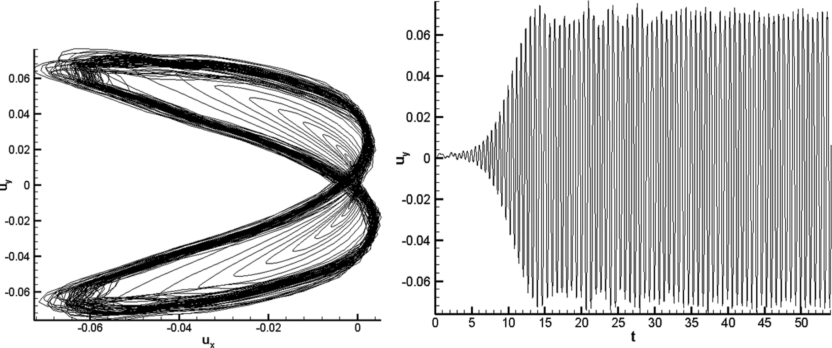Figure 10 shows the predicted y-displacements (m) of the flag tip compared to results found by Turek and Hron.¹⁰ The solution of Turek and Hron had a frequency and amplitude of 2 Hz and 0.08 m, respectively. The results from our FSI procedure give a displacement frequency of 1.7 Hz and amplitude of 0.07 m. The results of the current investigation also show higher harmonics as compared to the solution of Turek and Hron due to the increased fidelity of the current computational approach. Figure 11 shows the vertical tip displacement in the coarse mesh simulation.

Figure 9.

Trajectory trace of beam tip and y-displacement over entire simulation.

Figure 10.

Tip y-displacement comparison between fine mesh results in MBFLO2 and Turek and Hron.¹¹

Figure 11.

Tip y-displacement for coarse mesh.

Figure 12 shows instantaneous Mach number contours at the extrema of the tip displacement demonstrating the shedding in the flow and the beam movement. The results from this test case confirm the ability of the structural dynamics technique and the FSI approach in MBFLO2 to predict large structural displacements accurately.

Figure 12.

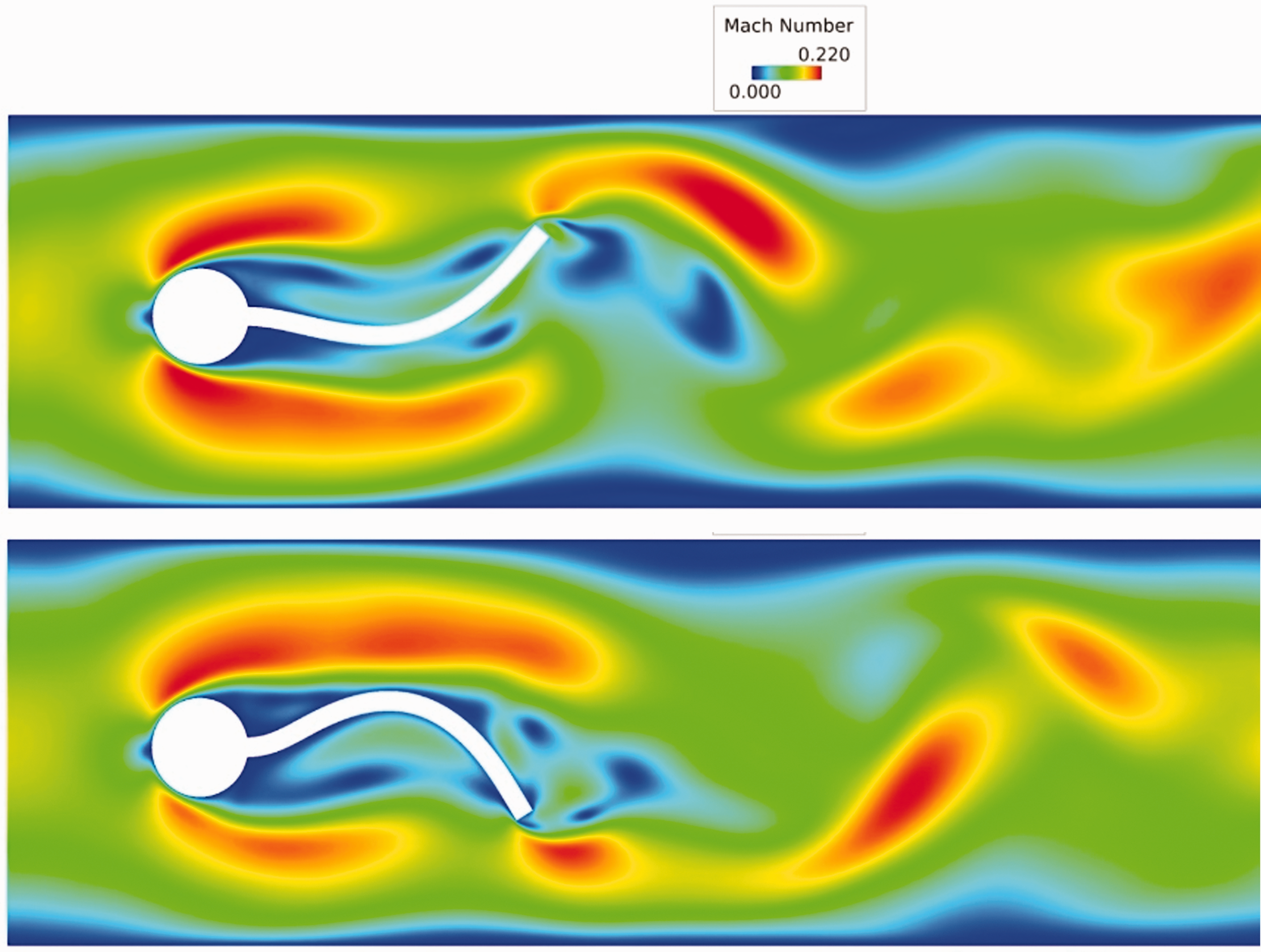
Cylinder flag Mach contours at extrema of displacements.

Figure 13 shows Fast Fourier transforms (FFTs) of the tip displacements of various cases ran with time steps of 0.0005, 0.00025, and 0.0001 for both the coarse and normal mesh. A stable solution was not obtainable for the coarse mesh and a time step of 0.0005. Fast Fourier transforms were performed over the entire time domain of the solution. Some cases were allowed to run for longer periods of time. The coarse mesh studies tend to have broader bandwidth about the dominant frequency than the nominal mesh as well as less pronounced higher modes. Similar patterns are seen with decreasing time step size.

Figure 13.

FFT of various cylinder flag simulations performed using MBFLO2.

Conclusion

A new and unique dual time-step, control–volume numerical technique has been developed for the solution of the two-dimensional structural dynamics conservation equations. Verification of the structural dynamics solution procedure shows excellent agreement with finite-element approach for a cantilever beam vibrating under gravity. The structural dynamics procedure was incorporated into a general, two-dimensional, conjugate Navier–Stokes solution procedure to create a fluid/thermal/structure interaction approach. The numerical techniques used in this multidisciplinary procedure were described. Verification of the FSI procedure was performed for a cylinder-flag combination in which the shedding from the cylinder forced oscillation in the flag. The results obtained show good agreement with the finite-element approach. The current procedure predicts a frequency of 1.7 Hz for the flag tip displacement whereas the finite-element results predicts a frequency of 2 Hz. Time-step and grid-refinement investigations indicate that the differences are due to higher-order modes predicted in the current procedure as opposed to the finite-element approach. These investigations also showed that the solution was essentially invariant with time-step size and grid refinement. The approach and results shown are a proof of concept of the technique, which is currently being extended to three dimensions.

Footnotes

Acknowledgements

The authors would like to thank the managers at AFRL and UTC for their support. The authors would also like to thank the managers of Intelligent Light for providing an academic license to the Fieldview scientific visualization system.

Declaration of Conflicting Interests

The author(s) declared no potential conflicts of interest with respect to the research, authorship, and/or publication of this article.

Funding

The author(s) disclosed receipt of the following financial support for the research, authorship, and/or publication of this article: This effort was partially supported by the Air Force Research Laboratory (AFRL) under Universal Technology Corporation (UTC) contract agreements 15–7900-0005–07-C1 and 16–7900-0004–06-C1 with Michele Puterbaugh as contract monitor and the University of California.

References

Nguyen

Trinh

Finite element model and vibration analysis of aero-elastic wing structures. In: 51st AIAA Aerospace Sciences Meeting including the New Horizons Forum and Aerospace Exposition, 2013. American Institute of Aeronautics and Astronautics. DOI: 10.2514/6.2013-58.

Jameson

A high-order spectral difference method for fluid-structure interaction on dynamic deforming meshes. In: 28th Applied Aerodynamics Conference, July 2010. American Institute of Aeronautics and Astronautics. DOI: 10.2514/6.2010-4932.

Harash

Yadykin

Abramovich

Nonlinear bending-torsion flutter experiments of a medium-aspect-ratio flexible wing model. Russ Aeronaut 2012; 55: 373–378.

Harash

, et al. Experiments on bending-torsion flutter in presence of piezoelectric actuators. In: 46th AIAA/ASME/ASCE/AHS/ASC Structures, Structural Dynamics, and Materials Conference, Austin, Texas, 18-21 April 2005. American Institute of Aeronautics and Astronautics.

Quan

Zheng

Aeroeleastic analysis of a flexible delta wing at high angle of attack. In: 31st AIAA Applied Aerodynamics Conference, June 2013. American Institute of Aeronautics and Astronautics.

Liu

Cai

Zhu

, et al. Calculation of wing flutter by a coupled fluid-structure method. J Aircraft 2001; 334–342.

Hoyniak

Clark

WS.

Aerodynamic damping predictions using a linearized Navier–Stokes analysis. In: ASME 1999 International Gas Turbine and Aeroengine Congress and Exhibition, Indianapolis, Indiana, USA, 7-10 June, 1999. ASME.DOI: 10.1115/99-GT-207.

Hall

Clark

WS.

A linearized analysis of unsteady transonic flows in turbomachinery. In: ASME 1993 International Gas Turbine and Aeroengine Congress and Exposition, Cincinnati, Ohio, USA, 24-27 May 1993. ASME. DOI: 10.1115/93-GT-094.

Gottfried

Fleeter

Aerodynamic damping predictions in turbomachines using a couples fluid-structure model. J Propul Power 2005; 21: 327–334. DOI: 10.2514/1.4720.

10.

Turek

Hron

Proposal for numerical benchmarking of fluid-structure interaction between and elastic object and laminar incompressible flow. Fluid-structure interaction modeling, simulation, optimisation. Berlin, Heidelberg: Springer, Vol. 53, pp. 371–385. DOI: 10.1007/3-540-34596-5_15.

11.

RH.

A multiple grid scheme for solving the Euler equations. AIAA J 1982; 20: 1565–1571. DOI: 10.2514/6.1981-1025.

12.

Dannenhoffer

JF.

Grid adaptation for complex two-dimensional transonic flows. CFDL-TR-87-10, Department of Aeronautics and Astronautics, Massachusetts Institute of Technology, August 1987, pp.120–143.

13.

Davis

Carter

JE.

Cascade viscous flow analysis using the Navier-Stokes equations.

AIAA J Propul Power 1987; 406–414. DOI: 10.2514/3.23005.

14.

Jameson

Time dependent calculations using multi-grid, with applications to unsteady flows past airfoils and wings. In: 10th Computational Fluid Dynamics Conference, 1991. American institute of Aeronautics and Astornautics. DOI: 10.2514/6.1991-1596.

15.

Steger

Sorenson

RL.

Automatic mesh-point clustering near a boundary in grid generation with elliptic partial differential equations. J Computat Phys 1979; 33: 405–410. DOI: 10.1016/0021-9991(79)90165-7.

16.

Thompson

Thames

Mastin

CW.

Automatic numerical generation of body-fitted curvilinear coordinate system for field containing any number of arbitrary two-dimensional bodies. J Computat Phys 1974; 15: 299–319. DOI: 10.1016/0021-9991(74)90114-4.

Procedure for 2D fluid–structure interaction simulation