Splitting spectral element method for fractional reaction-diffusion equations

Abstract

In this paper, we propose a second-order operator splitting spectral element method for solving fractional reaction-diffusion equations. In order to achieve a fast second-order scheme in time, we decompose the original equation into linear and nonlinear sub-equations, and combine a quarter-time nonlinear solver and a half-time linear solver followed by final quarter-time nonlinear solver. The spatial discretization is eigen-decomposition based on spectral element method. Since this method gives a full diagonal representation of the fractional operator and gets an exponential convergence in space. We have an accurate and efficient approach for solving spacial fractional reaction-diffusion equations. Some numerical experiments are carried out to demonstrate the accuracy and efficiency of this method. Finally, we apply the proposed method to investigate the effect of the fractional order in the fractional reaction-diffusion equations.

Introduction

In recent years, the fractional partial differential equations are wining more and more scientific applications across a variety of fields including control theory, ¹ biology,^2,3 electrochemical processes, ⁴ finance, ⁵ etc. There have been many numerical methods for discretizing fractional operators and resolving fractional differential equations^6–11 etc. Splitting methods have been fruitfully used to solve large systems of partial differential equations.^12–14 Usually, it is very difficult to find the exact (analytical) solution of a given problem in practice. Thus, we can use numerical methods to obtain an approximate solution of the equations. There are many major benefits of operator splitting, including dimension reduction, problem simplification, preservation of any order accuracy in time, and computational speed-up for some complex problems (cf.^15–17 and the references therein). In this paper, we try to extend the splitting method for spacial fractional reaction-diffusion equations as follows

$$\frac{\partial u}{\partial t}=\mu {\mathcal{L}}^{\alpha }(u)+\mathcal{N}(u),(\mathit{x},t)\in \Omega \times (0,T)$$

(1)

$$u{|}_{\partial \Omega }=b(\mathit{x})$$

(2)

with $0<\alpha <1$ , where Ω is a bounded domain in ${\mathbb{R}}^2$ , μ is viscosity coefficient, the fractional operator is defined as ${\mathcal{L}}^{\alpha }=-{(-\Delta )}^{\alpha }$ and the nonlinear term $\mathcal{N}(u)=f(u)$ (e.g. in the Fisher-Kolmogorov equation ¹⁸ $f=ru(1-\frac{u}{K})$ , here r and K > 0 are variable coefficients depending on the space). The initial condition is given as $u_0(\mathit{x})=g(\mathit{x})$ .

The fractional Laplacian ${(-\Delta )}^{\alpha }$ in this paper is defined as follows

$${(-\Delta )}^{\alpha }u(\mathit{x},t)={\displaystyle \sum _{i=1}^{\infty }{\lambda }_i^{\alpha }}{u}_i(t){\varphi }_i(\mathit{x})$$

(3)

where ${({\lambda }_i,{\varphi }_i)}_{i=1}^{\infty }$ are the eigenpairs of the standard Laplacian $-\Delta$ with certainty boundary conditions and u has the expansion $u(\mathit{x},t)={\displaystyle {\sum }_{i=1}^{\infty }{u}_i}(t){\varphi }_i(\mathit{x})$ . Alternatively, the fractional operator ${(-\Delta )}^{\alpha }$ can be defined ¹⁹ through the Fourier transform

$$\stackrel{}{{(-\Delta )}^{\alpha }}u(\omega )={\omega }^{2\alpha }\widehat{u}(\omega )$$

(4)

where $\widehat{u}$ is the Fourier transform of u. ²⁰

The remainder of this paper is organized as follows. In next section, we describe the numerical method for the fractional reaction-diffusion equations, and provide the error estimation for the splitting scheme. Several numerical examples are given in ‘Numerical results’ section. We will apply our method to solve the fractional Allen-Cahn, Fisher-Kolmogorov, Gray-Scott and FitzHugh–Nagumo equations.^2,11,21 The numerical results show that our method is both efficient and highly accurate for solving fractional reaction-diffusion equations. We provide a short summary in the final section.

Numerical method

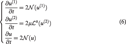
We introduce a second-order splitting scheme for solving the above reaction-diffusion equation (1) and derive the error estimation for the scheme in this section. Let L be the number of the time step to integrate up to final time T, then the time step $\Delta t=T/L,t_n=n\Delta t,t_{n+\frac{1}{4}}=t_n+\frac{\Delta t}{4}$ and $t_{n+\frac{3}{4}}=t_n+\frac{3\Delta t}{4}$ for $n=0,1,\dots ,L-1$ . We denote the time levels by superscripts $u^{n+1}=u(t_{n+1})$ and set initial condition $u^0=u_0(\mathit{x})$ . We look for solution of $u^{n+1},n=0,1,\dots ,L-1$

$$\{\begin{array}{l}\frac{\partial u^{(1)}}{\partial t}=2\mathcal{N}\left(u^{(1)}\right),t\in (t_n,t_{n+\frac{1}{4}})\hfill \\ \frac{\partial u^{(2)}}{\partial t}=2\mu {\mathcal{L}}^{\alpha }(u^{(2)}),t\in (t_{n+\frac{1}{4}},t_{n+\frac{3}{4}})\hfill \\ \frac{\partial u}{\partial t}=2\mathcal{N}(u),t\in (t_{n+\frac{3}{4}},t_{n+1})\hfill \end{array}$$

(5)

with the initial conditions in each sub-step $u^{(1)}(t_n)=u^n,u^{(2)}(t_{n+\frac{1}{4}})=u^{(1)}(t_{n+\frac{1}{4}})$ and $u(t_{n+\frac{3}{4}})=u^{(2)}(t_{n+\frac{3}{4}})$ respectively.

Remark 1. In particular case we can find the analytic solutions of the initial value problem with a given nonlinear term f(u), since the ordinary differential equations in the first sub-step and the third sub-step of the above scheme (5) are solvable. Alternatively, we solve a diffusion equation for the second sub-step with an efficiency way since the fractional operator is defined as (3).

Next, we will derive the error estimation for the above scheme (5). Here we have second-order convergence in time $O(\Delta t^2)$ which is the same as the splitting method used for standard reaction-diffusion equation (i.e. α = 1) in Harwood. ²²

Theorem 1. Given a semi-linear parabolic PDE, which can be written as $\frac{\partial u}{\partial t}=\mu {\mathcal{L}}^{\alpha }(u)+\mathcal{N}(u),$ where ${\mathcal{L}}^{\alpha }$ and $\mathcal{N}$ are linear and nonlinear operator upon u, respectively, the solutions to the set of split equations

$$\{\begin{array}{l}\frac{\partial u^{(1)}}{\partial t}=2\mathcal{N}(u^{(1)})\hfill \\ \frac{\partial u^{(2)}}{\partial t}=2\mu {\mathcal{L}}^{\alpha }(u^{(2)})\hfill \\ \frac{\partial u}{\partial t}=2\mathcal{N}(u)\hfill \end{array}$$

(6)

provide an $O(\Delta t^2)$ splitting accuracy when solved sequentially over the set of subintervals

$$\{(t_n,t_{n+\frac{1}{4}}],(t_{n+\frac{1}{4}},t_{n+\frac{3}{4}}],(t_{n+\frac{3}{4}},t_{n+1}]\}$$

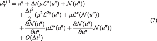
Proof. Using Taylor expansion at time step $t_{n+1}$ , the solution to the full problem (1)

$$\begin{array}{l}{u}_T^{n+1}=u^n+\Delta t(\mu {\mathcal{L}}^{\alpha }(u^n)+\mathcal{N}(u^n))\\ +\frac{\Delta t^2}{2}({\mu }^2{\mathcal{L}}^{2\alpha }(u^n)+\mu {\mathcal{L}}^{\alpha }(\mathcal{N}(u^n))\\ +\frac{\partial \mathcal{N}(u^n)}{\partial u^n}\mu {\mathcal{L}}^{\alpha }(u^n)+\frac{\partial \mathcal{N}(u^n)}{\partial u^n}\mathcal{N}(u^n))\\ +O(\Delta t^3)\end{array}$$

(7)

Combining the splitting equations (19) we have the following approximation, here we denote $u^{n+\frac{3}{4}}=u^{(2)}(t_{n+\frac{3}{4}}),u^{n+\frac{1}{4}}=u^{(1)}(t_{n+\frac{1}{4}})$ and I represents the identity operator for convenience. By using Taylor expansion

$$\begin{array}{l}{u}^{n+1}=u^{n+\frac{3}{4}}+\frac{\Delta t}{4}\frac{\partial u^{n+\frac{3}{4}}}{\partial t}+\frac{\Delta t^2}{32}\frac{{\partial }^2{u}^{n+\frac{3}{4}}}{\partial t^2}+O(\Delta t^3)\\ =u^{n+\frac{3}{4}}+\frac{\Delta t}{2}\mathcal{N}(u^{n+\frac{3}{4}})+\frac{\Delta t^2}{16}\frac{\partial \mathcal{N}(u^{n+\frac{3}{4}})}{\partial t}+O(\Delta t^3)\\ =u^{n+\frac{1}{4}}+\mu \Delta t{\mathcal{L}}^{\alpha }(u^{n+\frac{1}{4}})+\frac{\Delta t^2{\mu }^2}{2}{\mathcal{L}}^{2\alpha }(u^{n+\frac{1}{4}})\\ +\frac{\Delta t}{2}\mathcal{N}(u^{n+\frac{1}{4}}+\mu \Delta t{\mathcal{L}}^{\alpha }(u^{n+\frac{1}{4}})+O(\Delta t^2))\\ +\frac{\Delta t^2}{16}(\frac{\partial \mathcal{N}(u^{n+\frac{1}{4}})}{\partial t}+O(\Delta t))+O(\Delta t^3)\\ =u^{n+\frac{1}{4}}+\mu \Delta t{\mathcal{L}}^{\alpha }(u^{n+\frac{1}{4}})+\frac{\Delta t^2{\mu }^2}{2}{\mathcal{L}}^{2\alpha }(u^{n+\frac{1}{4}})\\ +\frac{\Delta t}{2}(\mathcal{N}(u^{n+\frac{1}{4}})+\mu \Delta t\frac{\partial \mathcal{N}(u^{n+\frac{1}{4}})}{\partial u^{n+\frac{1}{4}}}{\mathcal{L}}^{\alpha }(u^{n+\frac{1}{4}})+O(\Delta t^2))\\ +\frac{\Delta t^2}{8}\frac{\partial \mathcal{N}(u^{n+\frac{1}{4}})}{\partial u^{n+\frac{1}{4}}}\mathcal{N}(u^{n+\frac{1}{4}})+O(\Delta t^3)\end{array}$$

$$\begin{array}{l}=(I+\mu \Delta t{\mathcal{L}}^{\alpha }+\frac{\Delta t^2{\mu }^2}{2}{\mathcal{L}}^{2\alpha })(u^n+\frac{\Delta t}{4}\frac{\partial u^n}{\partial t}+\frac{\Delta t^2}{32}\frac{{\partial }^2{u}^n}{\partial t^2}+O(\Delta t^3))\\ +\frac{\Delta t}{2}(\mathcal{N}(u^n+\frac{\Delta t}{4}\frac{\partial u^n}{\partial t}+O(\Delta t^2))\\ +\Delta t(\frac{\partial \mathcal{N}(u^n)}{\partial u^n}+O(\Delta t))(\mu {\mathcal{L}}^{\alpha }(u^n)+O(\Delta t)))\\ +\frac{\Delta t^2}{8}(\frac{\partial \mathcal{N}(u^n)}{\partial u^n}+O(\Delta t))(\mathcal{N}(u^n)+O(\Delta t))+O(\Delta t^3)\\ =u^n+\Delta t(\mu {\mathcal{L}}^{\alpha }(u^n)+\frac{1}{2}\mathcal{N}(u^n))\\ +\frac{\Delta t^2}{2}({\mu }^2{\mathcal{L}}^{2\alpha }(u^n)+\mu {\mathcal{L}}^{\alpha }(\mathcal{N}(u^n))+\frac{1}{4}\frac{\partial \mathcal{N}(u^n)}{\partial u^n}\mathcal{N}(u^n))\\ +\frac{\Delta t}{2}\mathcal{N}(u^n)+\Delta t^2\left(\frac{1}{4}\frac{\partial \mathcal{N}(u^n)}{\partial u^n}\mathcal{N}(u^n)+\frac{1}{2}\frac{\partial \mathcal{N}(u^n)}{\partial u^n}\mu {\mathcal{L}}^{\alpha }(u^n)\right)\\ +\frac{\Delta t^2}{8}\frac{\partial \mathcal{N}(u^n)}{\partial u^n}\mathcal{N}(u^n)+O(\Delta t^3)\\ =u^n+\Delta t(\mu {\mathcal{L}}^{\alpha }(u^n)+\mathcal{N}(u^n))\\ +\frac{\Delta t^2}{2}({\mu }^2{\mathcal{L}}^{2\alpha }(u^n)+\mu {\mathcal{L}}^{\alpha }(\mathcal{N}(u^n))\\ +\frac{\partial \mathcal{N}(u^n)}{\partial u^n}\mu {\mathcal{L}}^{\alpha }(u^n)+\frac{\partial \mathcal{N}(u^n)}{\partial u^n}\mathcal{N}(u^n))+O(\Delta t^3)\end{array}$$

Where $u^{n+\frac{3}{4}}=u^{n+\frac{1}{4}}+\mu \Delta t{\mathcal{L}}^{\alpha }(u^{n+\frac{1}{4}})+\frac{\Delta t^2{\mu }^2}{2}{\mathcal{L}}^{2\alpha }(u^{n+\frac{1}{4}})+O(\Delta t^3)$ is derived from the second sub-step of the scheme (6). The $O(\Delta t^2)$ splitting error can be obtained by computing the $O(\Delta t^3)$ solution difference from this ordering as

$$|u_T^{n+1}-u^{n+1}|=O(\Delta t^3)$$

Thus, the symmetric splitting scheme results in second-order accuracy in time. The proof is complete. □

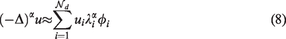
In previous work, we have developed a numerical method for computing fractional Laplacians on complex-geometry domains. ²³ By using the numerical eigenpairs $({\lambda }_i,{\varphi }_i)$ of the Laplace operator $-\Delta$ from the SEM solution, we can approximate the fractional Laplace operator as

$${(-\Delta )}^{\alpha }u\approx {\displaystyle \sum _{i=1}^{{\mathcal{N}}_d}{u}_i}{\lambda }_i^{\alpha }{\varphi }_i$$

(8)

where $u_i=({\varphi }_i,u),(·,·)$ represents inner product and ${\mathcal{N}}_d$ denotes the degree of freedom (DoF) which depends on the element number El and the polynomial degree N of the problem. The variational statement for the second sub-step of the scheme (5) reads as: Find $u_{{\mathcal{N}}_d}\in V_{{\mathcal{N}}_d}(\Omega ),\forall v\in V_{{\mathcal{N}}_d}(\Omega )$ so that

$$\left(\frac{\partial u_{{\mathcal{N}}_d}}{\partial t},v\right)=-2\mu ({(-{\Delta }_{{\mathcal{N}}_d})}^{\alpha }{u}_{{\mathcal{N}}_d},v)$$

(9)

where the time interval is $t\in (t_{n+\frac{1}{4}},t_{n+\frac{3}{4}}]$ and $V_{{\mathcal{N}}_d}(\Omega )=\text{span}\{{\varphi }_i,i=1,\dots ,{\mathcal{N}}_d\}$ and $u^{(2)}(t)$ in equation (5) is replaced by u(t) for convenience. The numerical solution is expanded as $u_{{\mathcal{N}}_d}={\displaystyle {\sum }_{i=1}^{{\mathcal{N}}_d}{u}_i}(t){\varphi }_i$ and the fractional operator ${(-{\Delta }_{{\mathcal{N}}_d})}^{\alpha }$ is defined as follows

$${(-{\Delta }_{{\mathcal{N}}_d})}^{\alpha }u={\displaystyle \sum _{i=1}^{{\mathcal{N}}_d}{\lambda }_i^{\alpha }}{u}_i(t){\varphi }_i$$

(10)

By the orthogonality of the eigenfunctions we obtain

$${\partial }_t{u}_i(t)=-2\mu u_i(t){\lambda }_i^{\alpha }$$

(11)

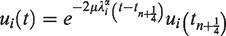
The solution of the above equations with initial condition $u_i(t_{n+\frac{1}{4}})$ is given as follows

$$u_i(t)=e^{-2\mu {\lambda }_i^{\alpha }\left(t-t_{n+\frac{1}{4}}\right)}{u}_i\left(t_{n+\frac{1}{4}}\right)$$

where $u_i(t_{n+\frac{1}{4}})={\displaystyle {\int }_{\Omega }u}(\mathit{x},t_{n+\frac{1}{4}}){\varphi }_{i}d\mathit{x}$ . Thus we obtain the analytic solution of (9)

$$u_{{\mathcal{N}}_d}(\mathit{x},t)={\displaystyle \sum _{i=1}^{{\mathcal{N}}_d}{e}^{-2\mu {\lambda }_i^{\alpha }\left(t-t_{n+\frac{1}{4}}\right)}}{u}_i\left(t_{n+\frac{1}{4}}\right){\varphi }_i$$

(12)

Numerical results

Fractional Allen-Cahn equation (verification of convergence results)

In order to test the convergence rates of the splitting scheme (5) for reaction-diffusion equations, we consider the fractional Allen-Cahn equation

$$\frac{\partial u}{\partial t}=-\mu {(-\Delta )}^{\alpha }u+u-u^3,(\mathit{x},t)\in \Omega \times (0,T),0<\alpha \le 1$$

(13)

with the Neumann boundary condition

$$\frac{\partial u(\mathit{x},t)}{\partial \mathit{n}}=0,\mathit{x}\in \partial \Omega$$

(14)

where the bounded domain $\Omega ={[-1,1]}^2$ and μ is the viscosity. The initial condition is given as

$$u(\mathit{x},0)=\sin (\pi x)\cos (2\pi y)$$

The corresponding nonlinear initial value problem for the Allen-Cahn equation is given as follows

$$\frac{\partial u}{\partial t}=2(u-u^3),s\in (t_{\xi },t]$$

(15)

here the initial condition is given as $u(t_{\xi })$ , here ξ is equal to n or $n+\frac{3}{4}$ at the n-th time step. The equation (15) can be integrated to obtain^24,25

$$u(s)=\frac{u(t_{\xi })}{\sqrt{e^{-4(s-t_{\xi })}+u{(t_{\xi })}^2(1-e^{-4(s-t_{\xi })})}},s\in (t_{\xi },t)$$

(16)

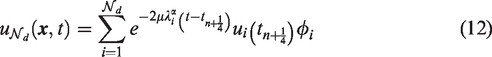
We set $\mu =0.01,T=2$ , the element number El = 64 and the polynomial degree N = 20 in each element such that the spatial discretization errors are negligible compared to the time discretization errors. Since the analytical solution is not available in this test, we choose the result obtained from the finest time step ${\tau }_0={10}^{-3}$ as our reference solution and compute the L² errors between the reference and the numerical solutions from several time steps $\Delta t$ , denote $e_1=\left|\right|u_{{\mathcal{N}}_d,{\tau }_0}-u_{{\mathcal{N}}_d,\Delta t}|{|}_{L^2(\Omega )}$ . We also use the numerical solution $u_{{\mathcal{N}}_d,\Delta t}^f$ as another reference solution, where $u_{{\mathcal{N}}_d,\Delta t}^f$ is computed by using the method we developed in Song et al., ²³ and denote $e_2=\left|\right|u_{{\mathcal{N}}_d,\Delta t}^f-u_{{\mathcal{N}}_d,\Delta t}|{|}_{L^2(\Omega )}$ . In Figure 1, we plot the L² errors e₁ and e₂ with different time steps $\Delta t$ for several fractional orders α. It is clear from Figure 1 that the scheme is second-order accurate method in time for any α. Moreover, the splitting scheme (5) is more accuracy than the scheme in Song et al. ²³ for $\alpha <1$ , since we solve the nonlinear equation (15) exactly in each time step. In Figure 2, we also show the spatial errors in semi-log scale for several α. The time step is $\Delta ={10}^{-3}$ and final time T = 1 in this test. It is observed that this method has exponential convergence rate for all α. Since the analytical solutions are not available in this test either, we choose the result obtained from the finest mesh N = 25 in each element as the reference solution and compute the L² errors between the reference and the numerical solutions from several polynomial degree N, denote $e=\left|\right|u_{25}-u_N|{|}_{L^2(\Omega )}$ .

Figure 1.

L² error as a function of $\Delta t$ in log-log scale with different fractional order α of the Allen-Cahn equation (13).

Figure 2.

L² error as a function of the polynomial degree N in semi-log scale with different fractional order α of the Allen-Cahn equation (13).

Fisher-Kolmogorov model

In this subsection, we consider the Fisher-Kolmogorov equation

$$\frac{\partial u}{\partial t}=-\mu {(-\Delta )}^{\alpha }u+ru(1-\frac{u}{K}),(\mathit{x},t)\in \Omega \times (0,T)$$

(17)

with the Dirichlet boundary condition

$$u(\mathit{x},t)=0,\mathit{x}\in \partial \Omega$$

(18)

where the bounded domain $\Omega =[-3,10]\times [-2,2],\hspace{0.17em}\mu =0.02,r=0.2$ , K(x, y) is a variable coefficient

$$K(x,y)=\{\begin{array}{l}{10}^{-7},\mathit{x}\in {\Omega }_b=[1,2]\times ([-2,0.2]\cup [0.4,2])\hfill \\ 1,\text{otherwise}\hfill \end{array}$$

(19)

In applications to biology, Ω _b represents a region where populations cannot grow, due to unfavorable environmental conditions. The geometry is a slitted barrier, through which the solution will eventually penetrate. K smoothly interpolate on the interface between Ω _b and outside region for our simulation. The initial condition is given as

$$u_0(\mathit{x})=0.8\exp (-25(x^2+y^2))$$

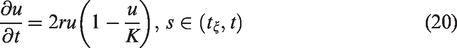
We consider the corresponding nonlinear initial value problem for the Fisher-Kolmogorov model as follows

$$\frac{\partial u}{\partial t}=2ru(1-\frac{u}{K}),s\in (t_{\xi },t)$$

(20)

here the initial condition is given as $u(t_{\xi })$ . The equation (20) can be integrated to obtain

$$u(s)=\frac{Ku(t_{\xi })e^{2r(s-t_{\xi })}}{K+u(t_{\xi })(e^{2r(s-t_{\xi })}-1)},s\in (t_{\xi },t)$$

(21)

We set $\Delta t=0.0002,T=90$ , the element number El = 117 and the polynomial degree N = 8 in each element to this simulation. Figure 3 shows the evolution of the solution for different fractional order $\alpha =1.0,0.85$ . These results conform to the results presented in Baeumer et al. ²⁶ Figure 3(a) shows the solution in the case of α = 1 (i.e. the classical reaction-diffusion equation) at t = 50, 70, 90. We can observe that the solution is very slow to penetrate the barrier. Next we change $\alpha =0.85$ to represent anomalous diffusion, and repeat the numerical simulation. Figure 3(b) shows the solution has penetrated significantly at time t = 70. Due to the strongly non-local character of the fractional operator, it is much easier for members of the population to cross (jump) over the barrier. Figure 4 shows the population masses versus time t for the cases $\alpha =1,0.85$ in two different regions ${\Omega }_1=[-3,1]\times [-2,2]$ and ${\Omega }_2=[2,10]\times [-2,2]$ . The population mass of the fractional case (i.e. $\alpha =0.85$ ) in ${\Omega }_2$ grows significantly faster than the classical case (i.e. α = 1) after time t = 40.

Figure 3.

Evolution of the solution corresponding to Fisher-Kolmogorov model. u contours are shown at times t = 50, 70, 90 from top to bottom. (a) $\alpha =1.0$ , (b) $\alpha =0.85$ .

Figure 4.

Population masses of the Fisher-Kolmogorov model versus t: $M_i={\displaystyle {\int }_{{\Omega }_i}u}d\mathit{x},i=1,2$ , here ${\Omega }_1=[-3,1]\times [-2,2]$ and ${\Omega }_2=[2,10]\times [-2,2]$ .

Gray-Scott model

In this subsection, we consider the Gray-Scott model. The Gray-Scott equations describe an autocatalytic reaction-diffusion process between two chemical constituents with concentrations u and v

$$\begin{array}{l}\frac{\partial u}{\partial t}=-{\mu }_u{(-\Delta )}^{\alpha }u-u{v}^2+c(1-u)\\ \frac{\partial v}{\partial t}=-{\mu }_v{(-\Delta )}^{\alpha }v+u{v}^2-(c+k)v\end{array}$$

(22)

with periodic boundary condition, the corresponding chemical reaction is as follows

$$\begin{array}{l}U+2V\to 3V\\ \hspace{1em}\hspace{0.17em}\hspace{1em}V\to P\end{array}$$

(23)

where the bounded domain $\Omega ={[-1,1]}^2,U,V$ and P are chemical species, u and v represent their concentrations, μ_u and μ_v are the diffusion rates, k represents the rate of conversion of V to P and c represents the rate of the process that feeds U and drains $U,V$ and P.

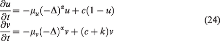
By splitting the linear terms of the reactive contribution into the linear system

$$\begin{array}{l}\frac{\partial u}{\partial t}=-{\mu }_u{(-\Delta )}^{\alpha }u+c(1-u)\\ \frac{\partial v}{\partial t}=-{\mu }_v{(-\Delta )}^{\alpha }v+(c+k)v\end{array}$$

(24)

the corresponding nonlinear system for $t\in (t_{\xi },t)$

$$\begin{array}{l}\frac{\partial u}{\partial t}=-2u{v}^2\\ \frac{\partial v}{\partial t}=2u{v}^2\end{array}$$

(25)

which has the conservation relation $u+v=u_0+v_0$ , where u₀ and v₀ are initial conditions. This allows the nonlinear system to be uncoupled to obtain $v_t=(u_0+v_0-v)v^2$ , which can be integrated to obtain

$$\{\begin{array}{l}u=u_0+v_0-v\hfill \\ v=\frac{u_0+v_0}{1+W_0\left(\frac{u_0}{v_0}\exp \right(\frac{u_0}{v_0}-2{(u_0+v_0)}^2(s-t_0)\left)\right)},\hfill \end{array}s\in (t_0,t)$$

(26)

where W₀ is the principal branch of the Lambert W function.^27,28 Writing equation (26) in terms of W₀ is only possible when $v_0\ne 0$ . In this simulation, the initial condition $v_0=0$ in the some regions of the domain. The Lambert W function can not be used in this case. Alternatively, we use fix-point iteration method for solving the nonlinear equation as follows

$$\frac{\partial v}{\partial t}=2(u_0+v_0-v)v^2$$

(27)

from the conservation relation $u_0+v_0=u+v$ .

We set $\Delta t=0.1,\Omega ={[0,1]}^2$ the element number El = 1600 and the polynomial degree N = 8 in each element to this simulation. The coefficients are given as ${\mu }_u=2\times {10}^{-5},{\mu }_v={\mu }_u/2$ , c = 0.03 and $k=k_1,k_2$ , where $k_1=0.055,k_2=0.063$ . For the ratio of diffusion coefficients ${\mu }_u/{\mu }_v>1$ , the model is known to generate different mechanisms of pattern formation depending on the values of the feed c and depletion k rates. We select k in a range in which the standard diffusion model is known to exhibit interesting dynamics. ³ The initial condition of the entire system is placed in the state $(u_0,v_0)=(1,0)$ , and the center plate ${(x-0.5)}^2+{(y-0.5)}^2\le {0.04}^2$ of the domain is perturbed to $(u_0,v_0)=(1/2,1/4)$ . Figure 5 shows the evolutions of the numerical solution v and summarizes the effects of the super-diffusion for the fractional Gray-Scott model. Since the evolutions of the numerical solution u is similar to that the v, we will not elaborate it in this paper. In Figure 5(a) to (c) with $\kappa =0.063$ , under the influence of the standard diffusion (α = 1), the Gray-Scott model exhibits patterns of mitosis. ³ However, in the super-diffusion case $\alpha =0.85,0.75$ , the way of the replication has a slight change and the dissociated spots become smaller. In Figure 5(d) to (f) with $\kappa =0.055$ , the Gray-Scott model with the normal diffusion ( $\alpha =1.0$ ) produces a circular wave propagating outward and forms a structured pattern shown in picture (d). Moreover, the reduction of the fractional order $\alpha =0.85$ effects the size of patterns with smaller spots. For smaller values of the fractional order $\alpha =0.75$ , a new process of nucleation of structures in the center and in the boundaries of the domain is observed, that then grow outward until the entire domain reaches its final steady state configuration. These results show the same phenomenon as the results in literature.^2,29

Figure 5.

Evolution of the solution v in Gray-Scott equation (22): (a)-(c) v contours are shown at times t = 2000, 4600, 5200, 6200, 7200, 9200, 12000, 18000 from top to bottom for three fractional orders $\alpha =1.0,0.85,0.75$ with k = 0.063; (d)-(f) v contours are shown at times t = 2000, 4600, 5200, 6200, 7200, 9200, 12000, 18000 from top to bottom for three fractional orders $\alpha =1.0,0.85,0.75$ with k = 0.055. (a) $\alpha =1.0$ , (b) $\alpha =0.85$ , (c) $\alpha =0.75$ , (d) $\alpha =1.0$ , (e) $\alpha =0.85$ , (f) $\alpha =0.75$ .

FitzHugh–Nagumo model

In the last subsection, we consider the fractional FitzHugh-Nagumo model as follows

$$\frac{\partial u}{\partial t}=-K_u{(-\Delta )}^{\alpha }u+u(1-u)(u-\sigma )-v$$

(28)

$$\frac{\partial v}{\partial t}=ϵ(\beta u-rv-\delta )$$

(29)

with homogeneous Neumann boundary condition on the bounded domain $\Omega ={[-1.25,1.25]}^2$ , where u is a normalized trans-membrane potential and v is a dimensionless time-dependent recovery variable, K_u is the diffusion coefficient. We set the parameters of the model: $K_u={10}^{-4},\sigma =0.1,ϵ=0.01,\beta =0.5,r=1$ and δ = 0, which is known to generate stable patterns in a system in the form of reentrant spiral waves. In order to illustrate the effect of varying fractional order α in the FitzHugh–Nagumo model, we take an initial condition as

$$\begin{array}{l}u(\mathit{x},0)=\{\begin{array}{l}1,x,y<0\hfill \\ 0,\text{otherwise}\hfill \end{array}\hfill \\ v(\mathit{x},0)=\{\begin{array}{l}0.1,y>0,\forall x\hfill \\ 0,\text{otherwise}\hfill \end{array}\hfill \end{array}$$

(30)

The time step in the numerical experiments is $\Delta t=0.1$ .

Figure 6 presents the stable rotation solutions of the FitzHugh-Nagumo model at t = 2000 for $\alpha =1,0.85,0.75$ . We find that as expected, the wave travels more slowly as fractional order decreases. The width of the excitation wavefront is markedly reduced for decreasing α, as is the wavelength of the system, with the domain being able to accommodate a larger number of wavefronts for smaller fractional order α. These visualizations are consistent with results presented in Bueno-Orovio et al. ² (Figure 3) for time up to t = 2000 for all α.

Figure 6.

Spiral waves in the FitzHugh-Nagumo model for varying α. (a) a = 1.0, (b) a = 0.85, (c) a = 0.75.

Summary

We develop a second-order operator splitting algorithm for solving reaction-diffusion equations with fractional operator. We analyze the discretization errors with benchmark solutions that show second-order convergence in time. We employ the spectral element method in space to solve the fractional diffusion equation. And we observe an exponential convergence in space. We investigate the effect of the fractional order for the different models, including the Allen-Cahn, Fisher-Kolmogorov, Gray-Scott and FitzHugh–Nagumo equations. Moreover, our method can be applied to the fractional reaction-diffusion models on complex-geometry domains, since the fractional Laplacian is defined as (8). We can use the spectral element method for solving the integer-order eigenvalue problem on complex-geometry domains. After we obtain the numerical eigenpairs of the eigenvalue problem, we can approach the fractional Laplace based on the eigenvalue decomposition on these domains. The approach is efficient as it does not require the solution of any linear systems since the eigenfunction decomposition leads naturally to a system of ODEs, which can be readily solved with standard methods.