The noise handling properties of the Talbot algorithm for numerically inverting the Laplace transform

Abstract

This paper examines the noise handling properties of three of the most widely used algorithms for numerically inverting the Laplace transform. After examining the genesis of the algorithms, their error handling properties are evaluated through a series of standard test functions in which noise is added to the inverse transform. Comparisons are then made with the exact data. Our main finding is that the for “noisy data”, the Talbot inversion algorithm performs with greater accuracy when compared to the Fourier series and Stehfest numerical inversion schemes as they are outlined in this paper.

The Laplace transform

The Laplace transform is an integral transform defined as follows.

Let f(t) be defined for $t\ge 0$ , then the Laplace transform of f(t) is given by

$$\mathcal{L}\left\{f\left(t\right)\right\}={\displaystyle {\int }_0^{\infty }f}\left(t\right)e^{-st}\text{d}t$$

(1)

Thus, $\mathcal{L}\left\{f\left(t\right)\right\}$ is a function of s denoted as F(s). The Laplace transform can be shown to exist for any function, which can be integrated over any finite interval $0<t<l$ for l > 0, and for which f(t) is of exponential order, i.e.

$$\left|f\left(t\right)\right|<M{e}^{at}$$

(2)

as $t\to \infty$ , where M and a are small real positive numbers.

Analytically, the inverse Laplace transform is usually obtained using the techniques of complex contour integration with the resulting set of standard transforms presented in tables. ¹

However, using the Laplace transform to obtain solutions of differential equations can lead to solutions in the Laplace domain, which are not easily invertible to the real domain by analytical means. Thus, numerical inversion techniques are used to convert the solution from the Laplace to the real domain.

The inverse Laplace transform and precision

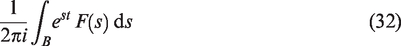
The recovery of the function f(t) is via the inverse Laplace transform, which is most commonly defined by the Bromwich integral formula

$${\mathcal{L}}^{-1}\left\{F\left(s\right)\right\}=f\left(t\right)=\frac{1}{2\pi i}{\displaystyle {\int }_{u-i\infty }^{u+i\infty }F}\left(s\right)e^{st}\text{d}s$$

(3)

for some $u\in \mathbb{ℝ}$ . ¹

The choice of s in equation (1) and so in equation (3) is not an arbitrary one. If we choose s such that it lies on the positive real axis, we are treating the solution of equation (3) as a positive real integral equation. The problem here is that the inverse problem is known to be ill-posed meaning that small changes in the values of F(s) can lead to large errors in the values for f(t). ²

Hence, when Laplace transform methods are used in finding numerical solutions to partial differential equations, the corresponding inversion methods can be highly sensitive to the inevitable noisy data that arises in their computation via truncation and round off error, a process that is exacerbated in nonlinear schemes. Abate and Valko ³ have shown that to some extent these errors can be curtailed by working in a multi-precision environment, however, as we show in the “Tests” section later, a small amount of noise in the data can significantly perturb the solution. When this is the case, it becomes difficult for unlimited precision to aid in the convergence of the algorithm to the correct solution.

The algorithms

There are over 100 algorithms available for inverting the Laplace transform with numerous comparative studies. Examples include Duffy, ² Narayanan and Beskos, ⁴ Cohen ⁵ and, perhaps, the most comprehensive by Davies and Martin. ⁶ However, for the purposes of this investigation we apply our tests using “Those algorithms that have passed the test of time”, ³ this is because these algorithms are reported to give the most accurate results on the widest variety of functions.^2,6 These fall into four groups:

Fourier series expansion.

Combination of Gaver functionals.

Laguerre function expansion.

Deformation of the Bromwich contour.

Derivations of particular versions of these algorithms are given in the sections which follow. In the upcoming sections, we examine the Stehfest algorithm, which is a widely used version of the Gaver functionals and the Talbot algorithm that uses a particular deformation of the Bromwich contour.

However, for now we do not run our tests using the Laguerre function expansion. While we do intend to investigate this method later on in our work, our choices in this work have been made based on the ease of implementation of the inversion method—an issue connected to parameter choice and control. The Laguerre method requires more than two parameters to effectively compute the desired transform, while the other three methods can perform reasonably well when defined using just the one parameter.

The Fourier series method

In their survey of algorithms for inverting the Laplace transform, Davies and Martin ⁶ note that the Fourier series method without accelerated convergence gives good accuracy on a wide variety of functions. Since the Laplace transform is closely related to the Fourier transform, it is not surprising that inversion methods based on a Fourier series expansion would yield accurate results. In fact, the two-sided Laplace transform can be derived from the Fourier transform in the following way. We can define the Fourier transform as

$$\mathcal{F}\left\{f\left(t\right)\right\}={\displaystyle {\int }_{-\infty }^{\infty }f}\left(t\right)e^{-2\pi i\nu t}\text{d}t$$

(4)

Then letting $v=2\pi \nu$ we have

$$\mathcal{F}\left\{f\left(t\right)\right\}={\displaystyle {\int }_{-\infty }^{\infty }f}\left(t\right)e^{-ivt}\text{d}t$$

(5)

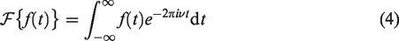
This Fourier transform exists provided f(t) is an absolutely integrable function, i.e.

$${\displaystyle {\int }_{-\infty }^{\infty }|}f\left(t\right)|\text{d}t<\infty$$

(6)

As many functions do not satisfy condition (6), f(t) is multiplied by the exponential dampening factor $e^{-ut}$ thus

$$F\left\{f\left(t\right)e^{-ut}\right\}={\displaystyle {\int }_{-\infty }^{\infty }f}\left(t\right)e^{-ivt}{e}^{-ut}\text{d}t$$

(7)

and letting $s=u+iv$ we obtain the two-sided Laplace Transform of f(t) as

$$\mathcal{F}\left\{f\left(t\right)e^{-ut}\right\}=\mathcal{L}\left\{f\left(t\right)\right\}={\displaystyle {\int }_{-\infty }^{\infty }{e}^{-st}}f\left(t\right)\text{d}t$$

(8)

LePage ⁷ noted that the integral given by equation (8) can be written in two parts as follows

$${\displaystyle {\int }_{-\infty }^{\infty }{e}^{-st}}f\left(t\right)\text{d}t={\displaystyle {\int }_{-\infty }^0{e}^{-st}}f\left(t\right)\text{d}t+{\displaystyle {\int }_0^{\infty }{e}^{-st}}f\left(t\right)\text{d}t$$

(9)

The second term in the above expression is referred to as the one-sided Laplace transform or simply the Laplace transform. Thus, s is defined as a complex variable in the definition of the Laplace transform.

As before the inverse Laplace transform is given as

$$f\left(t\right)=\frac{1}{2\pi i}{\displaystyle {\int }_{u-i\infty }^{u+i\infty }{e}^{st}}F\left(s\right)\text{d}s$$

(10)

With $s=u+iv$ in equation (10) this leads to the result

$$\begin{array}{c}f\left(t\right)=\frac{2e^{ut}}{\pi }{\displaystyle {\int }_0^{\infty }[\text{Re}\left\{F\left(u+iv\right)\right\}\cos \left(vt\right)}\\ -\text{Im}\left\{F(u+iv)\right\}\sin \left(vt\right)]\text{d}v\end{array}$$

(11)

Equations (1) and (11) can be replaced by the cosine transform pair

$$\text{Re}\left\{F\left(u+iv\right)\right\}={\displaystyle {\int }_0^{\infty }{e}^{-ut}}f\left(t\right)\cos \left(vt\right)\text{d}t$$

(12)

$$f\left(t\right)=\frac{2e^{ut}}{\pi }{\displaystyle {\int }_0^{\infty }\text{Re}}\left\{F\left(u+iv\right)\right\}\cos \left(vt\right)\text{d}v$$

(13)

or by the sine transform pair

$$\text{Re}\left\{F\left(u+iv\right)\right\}=-{\displaystyle {\int }_0^{\infty }{e}^{-ut}}f\left(t\right)\sin \left(vt\right)\text{d}t$$

(14)

$$f\left(t\right)=-\frac{2e^{ut}}{\pi }{\displaystyle {\int }_0^{\infty }\text{Im}}\left\{F\left(u+iv\right)\right\}\sin \left(vt\right)\text{d}v$$

(15)

Dunbar and Abate ⁸ applied a trapezoid rule to equation (13) resulting in the Fourier series approximation

$$f\left(t\right)\approx \frac{2e^{ut}}{T}\left[\frac{1}{2}F\left(u\right)+{\displaystyle \sum _{k=1}^{\infty }\text{Re}}\left\{F\left(u+\frac{k\pi i}{T}\right)\right\}\cos \left(\frac{k\pi t}{T}\right)\right]$$

(16)

where f(t) is expanded in the interval $0\le t<T$ . For faster computation, Simon and Stroot ⁹ proposed the following version of equation (16)

$$f\left(t\right)\approx \frac{e^{ut}}{t}\left[\frac{1}{2}F\left(u\right)+{\displaystyle \sum _{k=1}^{\infty }\text{Re}}\left\{F\left(u+\frac{k\pi i}{t}\right)\right\}{\left(-1\right)}^k\right]$$

(17)

This series can be summed much faster than equation (16) as there are no cosines to compute. ¹⁰ This algorithm is relatively easy to implement with u being the only real varying parameter.

However, as pointed out by Crump ¹¹ for the expression in equation (17), the transform F(s) must now be computed for a different set of s-values for each distinct t. Since this type of application occurs often in practice in which the numerical computation of F(s) is itself quite time consuming, this may not be an economical inversion algorithm to use. These drawbacks to some extent can be overcome by using the fast Fourier transform techniques.^10,12

Crump ¹¹ also extends this method to one of faster convergence by making use of the already computed imaginary parts. There are several other acceleration schemes for example, those outlined by Cohen; ⁵ however, these acceleration methods in general require the introduction of new parameters, which for the purpose of this investigation we wish to avoid.

The Stehfest algorithm

Davies and Martin ¹³ cite the Stehfest ¹⁴ algorithm as providing accurate results on a wide variety of test functions. Since that time, this algorithm has become widely used for inverting the Laplace transform, being favored due its reported accuracy and ease of implementation.

Here, we give a brief overview of the evolution of the algorithm from a probability distribution function to the Gaver functional whose asymptotic expansion leads to an acceleration scheme which yields the algorithm in its most widely used form.

Gaver ¹⁵ investigated a method for obtaining numerical information on the time dependent behavior of stochastic processes, which often arise in queuing theory. The investigation involved examining the properties of the three parameter class of density functions namely

$$p_{n,m}\left(a;t\right)=\frac{\left(n+m\right)!}{n!\left(m-1\right)!}{\left(1-e^{-at}\right)}^{n}a{e}^{-mat}$$

(18)

with $n,m\in \mathbb{N}.$ After the binomial expansion of the term ${\left(1-e^{-at}\right)}^n$ , Gaver went on to find the expectancy $E\left[f\left(T_{n,m}\right)\right]$ , where $T_{n,m}$ is the random variable with density (18). From this, Gaver was able to express the inverse Laplace transform in terms of the functional

$$f_{n,m}\left(t\right)=\frac{\ln 2}{t}\frac{\left(n+m\right)!}{n!\left(m-1\right)!}{\displaystyle \sum _{j=0}^n\left(\begin{array}{c}n\\ k\end{array}\right)}{\left(-1\right)}^{k}F\left(\left(k+m\right)\frac{\ln 2}{t}\right)$$

(19)

with certain conditions on n and m, Gaver makes n = m and expresses equation (19) as

$$f_n\left(t\right)=\frac{\ln 2}{t}\frac{\left(2n\right)!}{n!\left(n-1\right)!}{\displaystyle \sum _{k=0}^n\left(\begin{array}{c}n\\ k\end{array}\right)}{\left(-1\right)}^{k}F\left(\left(k+n\right)\frac{\ln 2}{t}\right)$$

(20)

While the expression in equation (20) can be used to successfully invert the Laplace transform for a large class of functions, its rate of convergence is slow.^2,13 However, Gaver ¹⁵ has shown that equation (20), with $a=\frac{\ln 2}{t}$ has the asymptotic expansion

$$f_n\left(t\right)\approx f\left(\frac{\ln 2}{a}\right)+\frac{{\alpha }_1}{n}+\frac{{\alpha }_2}{n^2}+\frac{{\alpha }_3}{n^3}+\cdots ,$$

(21)

where the α_j’s are constant coefficients in the asymptotic series. Hence, equation (21) converges to the limit

$$\underset{n\to \infty }{f_n\left(t\right)}=f\left(\frac{\ln 2}{a}\right)$$

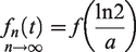
For the conditions on m and n and justification for the substitution for a referred to the above, see Gaver. ¹⁵ This asymptotic expansion provides scope for applying various acceleration techniques enabling a more viable application of the basic algorithm.

Stehfest’s acceleration scheme

For the purposes of the following Stehfest’s derivation it will be convenient to rewrite equation (20) as

$$f_n\left(t\right)=F_n=\frac{\left(2n\right)!a}{n!\left(n-1\right)!}{\displaystyle \sum _{k=0}^n\left(\begin{array}{c}n\\ k\end{array}\right)}{\left(-1\right)}^{k}F\left(\left(k+n\right)a\right)$$

(22)

Stehfest ¹ begins by supposing we have N values for $F[(k+n)a]$ with F(a), F(2a), F(3a), … .F(Na) for N even. Using equation (22), we can then determine $\frac{N}{2}$ values $F_1,F_2,\mathrm{\dots },F_{N/2}$ . Now each of these $N/2$ values satisfy the asymptotic series in equation (21) with the same coefficients.

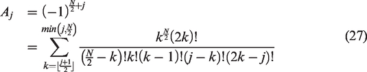
As pointed out by Stehfest, ¹ the α_j’s are the same for each of the above expansions and by using a suitable linear combination, the first ( $\frac{N}{2}-1$ ) error terms in equation (21) can be eliminated. That is

$$f\left(\frac{\ln 2}{a}\right)={\displaystyle \sum _{n=1}^{\frac{N}{2}}}{a}_n{F}_{(\frac{n}{2}+i-1)}+O\left(\frac{1}{N^{\frac{N}{2}}}\right)$$

(23)

which may be achieved by selecting the coefficients to satisfy

$${\displaystyle \sum _{n=1}^{\frac{N}{2}}}{a}_n\frac{1}{{\left(\frac{N}{2}+1-n\right)}^k}={\delta }_{k,0}k=1,\mathrm{\dots },N/2-1$$

(24)

$$a_n=\frac{{\left(-1\right)}^{n-1}}{\left(\frac{N}{2}\right)!}\left(\begin{array}{c}\frac{N}{2}\\ n\end{array}\right)n\left\{{\left(\frac{N}{2}+1-n\right)}^{\frac{N}{2}-1}\right\}$$

(25)

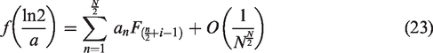
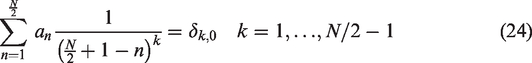
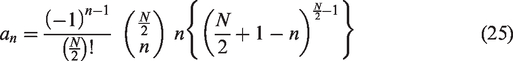
Finally, Stehfest ¹⁴ substituted these results into equation (23) and obtained the inversion formula

$$f\left(t\right)\approx \frac{\ln 2}{t}{\displaystyle \sum _{j=1}^N{A}_j}F\left(\frac{j\ln 2}{t}\right)$$

(26)

for N even.

$$\begin{array}{l}{A}_j={\left(-1\right)}^{\frac{N}{2}+j}\\ ={\displaystyle \sum _{k=\lfloor \frac{j+1}{2}\rfloor }^{min(j,\frac{N}{2})}\frac{k^{\frac{N}{2}}\left(2k\right)!}{\left(\frac{N}{2}-k\right)!k!\left(k-1\right)!\left(j-k\right)!\left(2k-j\right)!}}\end{array}$$

(27)

The Talbot algorithm

Equations (4) to (8) showed that the Laplace transform can be seen as a Fourier transform of the function

$$e^{-ut}f\left(t\right),t>0$$

(28)

i.e.

$$\mathcal{F}\left\{e^{-ut}f\left(t\right)\right\}=\mathcal{L}\left\{f\left(t\right)\right\}=F\left(s\right)$$

(29)

Hence, the Fourier transform inversion formula can be applied to recover the function, thus

$${\mathcal{F}}^{-1}\left\{F\left(s\right)\right\}=e^{-ut}f\left(t\right)=\frac{1}{2\pi }{\displaystyle {\int }_{-\infty }^{\infty }F}\left(s\right)e^{ivt}\text{d}v$$

(30)

as $s=u+iv$ we have that $ds=idv$ and so

$$f\left(t\right)=\frac{1}{2\pi i}{\displaystyle {\int }_{u-i\infty }^{u+i\infty }F}\left(s\right)e^{st}\text{d}s$$

(31)

This result provides a direct means of obtaining the inverse Laplace transform. In practice, the integral in equation (31) is evaluated using contour integration

$$\frac{1}{2\pi i}{\displaystyle {\int }_B{e}^{st}}F\left(s\right)\text{d}s$$

(32)

with B denoting the Bromwich contour. ¹ The contour is chosen so that it encloses all the possible singularities of F(s). The idea of the contour is introduced so that the residue theorem can be used to evaluate the integral. However, when f(t) is to be calculated using numerical quadrature it may be more appropriate to devise a new contour. To ensure the convergence of equation (32), we may wish to control the growth of the magnitude of the integrand e^st by moving the contour to the left so giving the real part of s a large negative component.^3,16However, the deformed contour must not be allowed to pass through any singularities of F(s). This is to ensure that the transform is analytic in the region to the right of $B$ .

Derivation of the fixed Talbot contour

In the derivation that follows Abate and Valko ³ and Murli and Rizzardi ¹⁶ are used as the primary basis for extending the explanation of the derivation of the Talbot algorithm for inverting the Laplace transform.

Abate and Valko ³ begin with the Bromwich inversion integral along the Bromwich contour B with the substitution

$$F\left(s\right)=\frac{1}{s^{\alpha }},\alpha >0$$

(33)

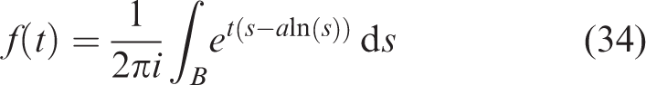
So f(t) can be expressed as

$$f\left(t\right)=\frac{1}{2\pi i}{\displaystyle {\int }_B{e}^{t\left(s-a\ln \left(s\right)\right)}}\text{d}s$$

(34)

with $a=\frac{\alpha }{t}$ in equations (33) and (34). As pointed out by Abate and Valko, ³ numerically evaluating the integral in equation (34) is difficult due to the oscillatory nature of the integrand.

However, this evaluation can be achieved by deforming the contour B into a path of constant phase, thus eliminating the oscillations in the imaginary component. These paths of constant phase are also paths of steepest decent for the real part of the integrand.^3,16,17

There are, in general, a number of contours for which the imaginary component remains constant and so we choose one on which the real part attains a maximum on the interior (a saddle point) and this occurs at $g\prime (s)=0$ at some point on the contour. At these saddle points, the $Im\left\{g\left(s\right)\right\}=0$ . ¹⁶ Here

$$g\left(s\right)=s-a\text{ln}s$$

(35)

in equation (34). Thus we have

$$g\prime \left(s\right)=1-\frac{a}{s}$$

(36)

so the stationary point occurs when s = a.

With $s=u+iv$ we have

$$\text{Im}\left\{u+iv-a\text{ln}\left(u+iv\right)\right\}=0$$

(37)

Expressing u + iv as $R{e}^{i\theta }$ we have

$$\text{Im}\{\left(u-a\text{ln}\left(R\right)\right)+i\left(v-a\theta \right)\}=0$$

(38)

then

$$v=a\theta$$

(39)

and as

$$\tan \left(\theta \right)=\frac{v}{u}$$

(40)

Then^3,18

$$u=a\theta \cot \left(\theta \right)$$

(41)

With $v=a\theta$ , then s can be parametrized to Talbots contour

$$s\left(\theta \right)=a\theta \left(\cot \left(\theta \right)+i\right),-\pi <\theta <+\pi$$

(42)

Conformal mapping of the Talbot contour

While the above parametrization can be used as a basis for inverting the Laplace transform, we proceed with the algorithm’s development via a convenient conformal mapping as follows. Expressing $\cot (\theta )$ as

$$\cot \theta =\frac{i\left(e^{i\theta }+e^{-i\theta }\right)}{\left(e^{i\theta }-e^{-i\theta }\right)}$$

(43)

Then

$$\theta \cot \theta +i\theta$$

(44)

is

$$\frac{2i\theta }{1-e^{-2i\theta }}$$

(45)

with $z=2i\theta$ then (45) becomes

$$\frac{z}{1-e^{-z}}$$

(46)

The function

$$S\left(z\right)=\frac{z}{1-e^{-z}}$$

(47)

maps the closed interval $M=\left[-2\pi i,2\pi i\right]$ on the imaginary z-plane onto the curve L in the s plane giving the integral

$$f\left(t\right)=\frac{1}{2\pi i}{\displaystyle {\int }_{\mathcal{L}}F}\left(s\right)e^{st}\text{d}s$$

(48)

For details of this transformation, one can refer to the study of Logan. ¹⁹

Next we follow the procedure as adopted by Logan ¹⁹ for numerically integrating equation (48). With $s=S\left(z\right)$ equation (48) becomes

$$f\left(t\right)=\frac{1}{2\pi i}{\displaystyle {\int }_{M}F}\left(S\left(z\right)\right)e^{S(z)t}{S}^{\prime }\left(z\right)\text{d}z$$

(49)

where

$$S\prime \left(z\right)=\frac{1-\left(1+z\right)e^{-z}}{{\left(1-e^{-z}\right)}^2}$$

(50)

For convenience we write

$$f\left(t\right)=\frac{1}{2\pi i}{\displaystyle {\int }_{M}I}\left(z,t\right)\text{d}z$$

(51)

where

$$I\left(z,t\right)=F\left(S\left(z\right)\right)e^{S(z)t}{S}^{\prime }\left(z\right)$$

(52)

The integral in equation (51) is then rotated by $\frac{\pi }{2}$ and so the interval of integration is now real and becomes $[-2\pi ,2\pi ]$ . Then, we use the trapezoid rule with n odd and $w=-iz$ to obtain

$$f\left(t\right)\cong \frac{1}{n}\left\{(I\left(2\pi i\right)+T\left(-2\pi i\right)+2{\displaystyle \sum _{j=1}^{n-1}I}\left(i{w}_j\right)\right\}$$

(53)

where

$$w_j=2\pi \left(\frac{2j}{n}-1\right)$$

(54)

and we note that $I\left(2\pi i\right)=I\left(-2\pi i\right)=0$ . ¹⁹

The regularization properties of the Talbot algorithm

Despite the intricacies of deriving the Talbot algorithm we have found it to be a relatively easy algorithm to implement. Also, the tests we have carried out so far show that the algorithm performs to a high degree of accuracy. Moreover, the algorithm converges much faster than the Fourier series method without requiring the use of any acceleration schemes. Additionally, in the form in which we have used it, there is only one parameter to control. But perhaps its greatest strength is the fact that we have found that it is able to handle noisy data (of magnitude outlined below) with little growth in the corresponding error. As shown by us, this is not the case for either the Fourier series or the Stehfest inversion algorithms presented above. Moreover, this “regularization property” does not exist for many of the numerical inversion schemes as indicated by Egonmwan. ²⁰ For most algorithms, this is generally overcome by constructing some regularization scheme, which then needs to be attached on to the inversion algorithm(s) of choice. This, of course, increases the complexity of the inversion process involving new parameters thus requiring even greater knowledge of the desired solution. This is even more so if the scheme also involves some additional accelerated convergence process.

As pointed out earlier, the perturbation in the numerical schemes is a consequence of the inversion being carried out on the real axis in the complex plane. The inclusion of complex arithmetic in the Talbot scheme enormously diminishes this perturbation. Of great importance here too is that the “regularization properties” of the Talbot algorithm means that very good performance can be obtained on many of the test functions without the necessity for multi-precision.

Egonmwan ²⁰ examined regularized and collocation methods for the numerical inversion of the Laplace transform, which involve Tikhonov ¹⁸ based methods. This is then applied to the Stehfest ¹⁴ and Piessens ²¹ methods on various standard test functions for both exact F(s) and noisy ( $F(s)+\mathrm{ϵ}$ ) data, where â denotes the magnitude of noise added.

For the Stehfest, ¹⁴ Piessens, ⁴ and the regularized method, Egonwan ²⁰ added noise of a magnitude ${10}^{-3}\times U(1,0)$ where U(1, 0) is a random number between 1 and 0 to the Laplace transform values. Commenting on his results, Egonwan notes “the Gaver Stehfest method gave very nice approximate solutions for a wide range of functions. However, it completely failed in the presence of noisy data. In the case of exact data, the method produced better numerical approximations when compared to the Piessins and the regularized collocation methods. However, the Piessins method gave better results than the regularized collocation method in the case of exact data”.

In other words, methods that performed well for exact data did not do well for noisy data and the regularized collocation method failed for exact data. Thus, to use such regularized methods requires some a priori knowledge of the magnitude of the noise involved and by implication a better estimation of the solution than might be otherwise possible.

Tests

Table 1 lists the functions together with a variety of properties for the purpose of testing the noise handling capability of the three inversion algorithms employed.

Table 1.

Test functions.

No.	F(s)	f(t)	Function type
1	$\frac{s}{{\left(s^2+1\right)}^2}$	$0.5t\sin (t)$	Oscillating increasing
2	$\frac{1}{{\left(s+1\right)}^2}$	$t{e}^{-t}$	Exponentially decreasing
3	$\frac{1}{s^5}$	$\frac{1}{24}{t}^4$	Increasing
4	$\frac{1}{\sqrt{s}}$	$\frac{1}{\pi t}$	With singularities
5	$\text{erf}\left\{\frac{2}{\sqrt{s}}\right\}$	$\frac{1}{\pi t}\sin \left(4\sqrt{t}\right)$	Oscillating with singularities
6	$\frac{1}{s^2-{0.5}^2}$	$\sinh \left(0.5t\right)$	Hyperbolic
7	$\frac{s^3}{s^4+4{(0.5)}^4}$	$\cos \left(0.5t\right)\cosh \left(0.5t\right)$	Combination of oscillating and hyperbolic
	$\frac{\ln s}{s}$	$-\left(\ln t+\gamma \right)$	Natural log

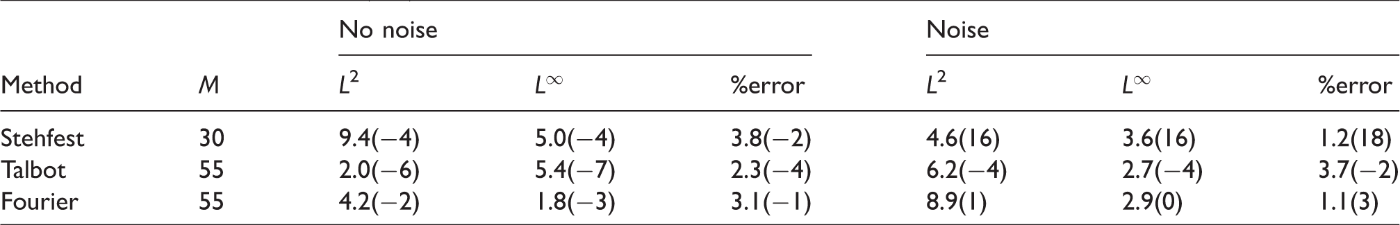
These functions are the same used by Egonmwan. ²⁰ This sample of test functions has a variety of properties, which we think forms a basis for testing the robustness of the noise handling properties of the inversion schemes. We use three error measures, the L² norm defined as

$${\mathcal{L}}^2=\sqrt{{\displaystyle \sum _{i=1}^{40}|}{f}_{numerical}\left(t_i\right)-f_{exact}\left(t_i\right){|}^2},i=\mathrm{1..40}$$

(55)

the ${\mathcal{L}}^{\infty }$ norm as

$${\mathcal{L}}^{\infty }=\max |f_{numerical}(t_i)-f_{exact}\left(t_i\right)|,i=\mathrm{1..40}$$

(56)

and the percentage error as

$$\max |\frac{f_{numerical}\left(t_i\right)-f_{exact}\left(t_i\right)}{f_{exact}\left(t_i\right)}\times 100|,i=1,\mathrm{..40.}$$

(57)

To give a good estimation of the errors involved we have sampled t over 40 points for t = 0.1 to 4. The L² norm is chosen as a measure, which averages out the error over the sample points while the ${\mathcal{L}}^{\infty }$ norm and the % error as defined above chooses the maximum error obtained for these measures. In all cases, the magnitude of noise added is ${10}^{-3}\times U(1,0)$ . The precision used for implementing the three algorithms is $1.8M$ where M is the number of weights for the Stehfest algorithm and 2M where M is the number of terms in the summation for the Talbot and the Fourier methods. The choice of these levels of precision is based on trial and error.

They are perhaps larger than they need to be but as our interest in this investigation is not on their efficiency but on their ability to handle noisy data we wanted to ensure that the precision played as little part as possible in assessing their performance. Thus, in cases where the extended precision decreases the accuracy of the noisy data we used the usual double precision for these inversions.

For functions which have sine, cosine, and hyperbolic properties we increased the weights for the Stehfest. This is because these functions require more weights and a corresponding increase in precision for the Stehfest method to produce accurate results. For the Fourier series method, we choose the parameter value of a = 4, with u = at in equation (17). Once again this choice is based on trial and error. We have found that this choice for a gives the best results for inverting the widest class of functions.

Results

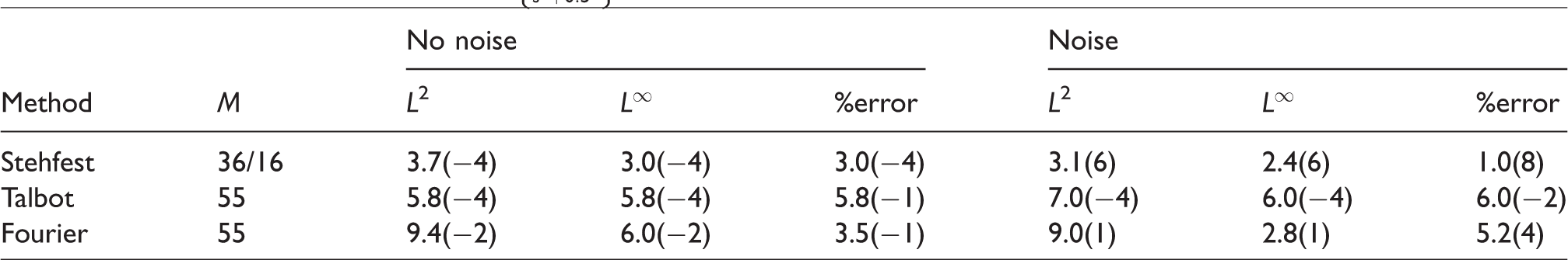
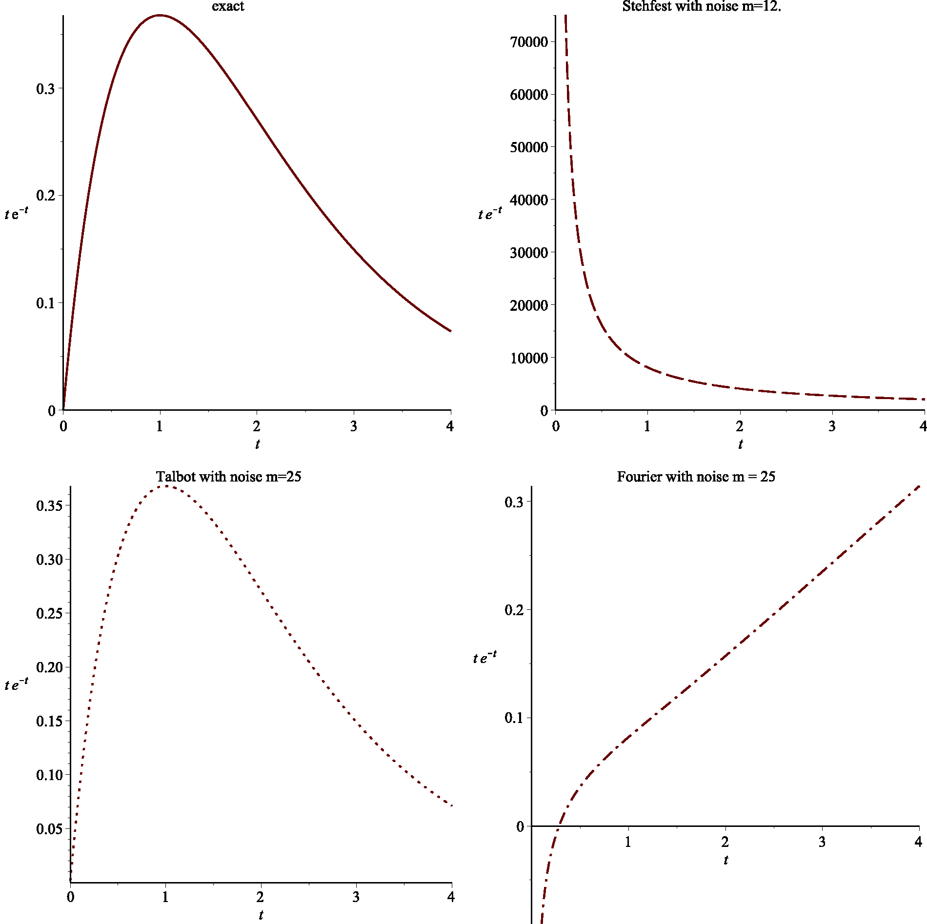
Tables 2 to 9 and Figures 1 to 4 show very good performance of the Talbot algorithm in handling noisy data. (For brevity, we have included only four graphical results for the eight functions using different weights as the performance of these functions with a higher number of weights are well illustrated in the tables.)

Table 2.

$f(t)=0.5t\sin (t)$ $=L^{-1}\left\{\frac{s}{{(s^2+1)}^2}\right\}$ .

		No noise			Noise
Method	M	L 2	$L^{\infty }$	%error	L 2	$L^{\infty }$	%error
Stehfest	30	9.4(−4)	5.0(−4)	3.8(−2)	4.6(16)	3.6(16)	1.2(18)
Talbot	55	2.0(−6)	5.4(−7)	2.3(−4)	6.2(−4)	2.7(−4)	3.7(−2)
Fourier	55	4.2(−2)	1.8(−3)	3.1(−1)	8.9(1)	2.9(0)	1.1(3)

Table 3.

$f(t)=t{e}^{-t}=L^{-1}\left\{\frac{1}{{(s+1)}^2}\right\}$ .

		No noise			Noise
Method	M	L 2	$L^{\infty }$	%error	L 2	$L^{\infty }$	%error
Stehfest	16	1.1(−4)	4.0(−5)	5.4(−1)	3.0(7)	2.4(7)	2.6(10)
Talbot	55	7.3(−6)	6.4(−6)	2.1(−3)	7.8(−4)	2.3(−4)	3.1(−1)
Fourier	55	3.6(−3)	1.0(−2)	4.9(−0)	1.1(0)	9.0(−1)	9.7(2)

Table 4.

$f\left(t\right)=\frac{1}{24}{t}^4=L^{-1}\left\{\frac{1}{{\left(s\right)}^5}\right\}$ .

		No noise			Noise
Method	M	L 2	$L^{\infty }$	%error	L 2	$L^{\infty }$	%error
Stehfest	16	6.7(−6)	3.0(−54)	2.8(−3)	3.8(3)	2.4(3)	1.1(12)
Talbot	55	3.8(−10)	3.4(−10)	5.1(−4)	2.3(−3)	8.8(−4)	1.5(−1)
Fourier	55	6.2(−1)	2.9(−1)	2.7(0)	7.6(0)	16.3(1)	2.5(3)

Table 5.

$f\left(t\right)=\frac{1}{\sqrt{\pi t}}=L^{-1}\left\{\frac{1}{\left(\sqrt{s}\right)}\right\}$ .

		No noise			Noise
Method	M	L 2	$L^{\infty }$	%error	L 2	$L^{\infty }$	%error
Stehfest	16	2.7(−8)	1.3(−8)	7.2(−7)	1.5(7)	1.2(7)	6.5(8)
Talbot	55	9.2(−2)	9.2(−3)	5.2(−2)	9.2(−2)	9.2(−3)	5.2(−2)
Fourier	55	6.2(−1)	2.9(−1)	2.7(0)	1.4(1)	6.3(0)	7.1(6)

Table 6.

$f\left(t\right)=\frac{1}{\pi t}\sin \left(4\sqrt{t}\right)=L^{-1}\left\{erf\left(\frac{2}{\sqrt{s}}\right)\right\}$ .

		No noise			Noise
Method	M	L 2	$L^{\infty }$	%error	L 2	$L^{\infty }$	%error
Stehfest	16	2.6(−4)	1.6(−4)	6.6(−1)	1.2(7)	9.6(6)	7.2(9)
Talbot	55	2.2(−2)	2.2(−2)	7.1(−1)	2.2(−1)	2.2(−2)	7.1(−1)
Fourier	55	1.8(1)	1.1(1)	4.3(3)	3.9(3)	2.2(3)	4.1(6)

Table 7.

$f\left(t\right)=\frac{\sinh \left(0.5t\right)}{0.5}=L^{-1}\left\{\frac{1}{s^2-{0.5}^2}\right\}$ .

		No noise			Noise
Method	M	L 2	$L^{\infty }$	%error	L 2	$L^{\infty }$	%error
Stehfest	36	9.8(−3)	9.2(−3)	2.1(−5)	2.6(7)	2.0(7)	7.0(6)
Talbot	55	7.2(−6)	7.2(−6)	4.6(−6)	4.5(−4)	3.1(−4)	7.6(−3)
Fourier	55	1.4(−1)	1.4(−1)	1.9(0)	1.7(1)	5.8(0)	3.4(2)

Table 8.

$f\left(t\right)=\cosh \left(0.5t\right)\cos \left(0.5t\right)=L^{-1}\left\{\frac{s^3}{s^4+{0.5}^2}\right\}$ .

		No noise			Noise
Method	M	L 2	$L^{\infty }$	%error	L 2	$L^{\infty }$	%error
Stehfest	36/16	3.7(−4)	3.0(−4)	3.0(−4)	3.1(6)	2.4(6)	1.0(8)
Talbot	55	5.8(−4)	5.8(−4)	5.8(−1)	7.0(−4)	6.0(−4)	6.0(−2)
Fourier	55	9.4(−2)	6.0(−2)	3.5(−1)	9.0(1)	2.8(1)	5.2(4)

Table 9.

$f\left(t\right)=-\left(\ln \left(t\right)+\gamma \right)=L^{-1}\left\{\frac{\ln s}{s}\right\}$ .

		No noise			Noise
Method	M	L 2	$L^{\infty }$	%error	L 2	$L^{\infty }$	%error
Stehfest	16	1.9(−8)	1.2(−7)	2.8(−5)	1.4(7)	1.8(7)	2.4(9)
Talbot	55	6.9(−3)	6.9(−3)	4.0(−1)	7.1(−3)	7.1(−3)	4.1(−1)
Fourier	55	8.6(−1)	8.3(−2)	4.0(3)	1.2(2)	3.8(2)	6.3(3)

Figure 1.

Numerical reconstruction of $f\left(t\right)=0.5t.\sin \left(t\right)=L^{-1}\left\{\frac{s}{{\left(s^2+1\right)}^2}\right\}$ .

Figure 2.

Numerical reconstruction of $f\left(t\right)=t{e}^{-t}=L^{-1}\left\{\frac{1}{{\left(s+1\right)}^2}\right\}$ .

Figure 3.

Numerical reconstruction of $f\left(t\right)=\frac{1}{24}{t}^4=L^{-1}\left\{\frac{1}{s^5}\right\}$ .

Figure 4.

Numerical reconstruction of $f\left(t\right)=\frac{1}{\pi t}=L^{-1}\left\{\frac{1}{\sqrt{s}}\right\}$ .

With the exception of the function $f(t)=\frac{1}{\sqrt{\pi t}}$ in Table 5 (for which the L² norm and ${\mathcal{L}}^{\infty }$ norm maintain their very small size), the error for the Talbot inversion diminishes considerably as a function of M. However, for both the Fourier series and the Stehfest inversion methods both measures of error increase as M increases.

In Table 6, we also observe that the recovery of the function $erf\left(\frac{2}{\sqrt{s}}\right)$ performs badly for the Fourier series method in both the noisy and noise free environment.

Table 8 includes two sets of weights for the Stehfest inversion algorithm. For the accurate inversion of sinusoidal functions, this algorithm requires more weights for increasing values of t, here for example we use 36 weights. However, when noise is added the accuracy decreases with the number of weight used, thus in this case for better performance we have used 16 weights.

Table 9 again shows the minimal error involved for the Talbot inversion when noise is added.

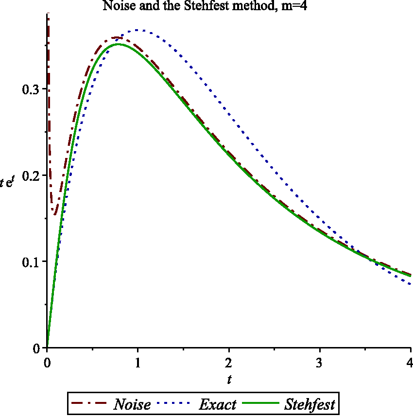
Figures 5 and 6 demonstrate that the Stehfest algorithm handles noisy data more accurately by decreasing the number of weights used. This is because the error generated in reconstructing the function from noisy data increases as the number of weights used rises. However, the accuracy achieved by decreasing the number of weights is not sufficient to justify such an approach for handling noisy data. Moreover, as we have stated a larger number of weights and the corresponding increase in precision is necessary for handling trigonometric and hyperbolic functions. We again note that no such considerations are necessary when employing the Talbot algorithm.

Figure 5.

Numerical reconstruction of $f\left(t\right)=0.5t.\sin \left(t\right)=L^{-1}\left\{\frac{s}{{\left(s^2+1\right)}^2}\right\}$ .

Figure 6.

Numerical reconstruction of $f\left(t\right)=0.5t.\sin \left(t\right)=L^{-1}\left\{\frac{s}{{\left(s^2+1\right)}^2}\right\}$ .

Conclusions

The results show that the Talbot algorithm handles the noisy data extremely well having very little impact on the final outcome. Both the Stehfest and the Fourier series methods fail to handle the noise. This is due to the fact that a significant part of the perturbation in these numerical schemes is a consequence of the inversion being carried out on the real axis in the complex plane. The inclusion of complex arithmetic in the Talbot scheme via the steepest decent path and the resulting elimination of the oscillations in the imaginary component enormously diminishes this perturbation. This has implications for implementing the LTFD method when solving nonlinear diffusion or time dependent parabolic partial differential equations, which can generate noisy data through a combination of measurement, truncation, and round-off error. Using the Talbot algorithm in these circumstances avoids additional complications such as having to devise regularized collocation methods to attain accurate solutions to these problems.