
Abstract
This paper proposes a numerical approach to the solution of the Fisher-KPP reaction-diffusion equation in which the space variable is developed using a purely finite difference scheme and the time development is obtained using a hybrid Laplace Transform Finite Difference Method (LTFDM). The travelling wave solutions usually associated with the Fisher-KPP equation are, in general, not deemed suitable for treatment using Fourier or Laplace transform numerical methods. However, we were able to obtain accurate results when some degree of time discretisation is inbuilt into the process. While this means that the advantage of using the Laplace transform to obtain solutions for any time t is not fully exploited, the method does allow for considerably larger time steps than is otherwise possible for finite-difference methods.
Keywords
Fisher’s equation
Fisher
1
suggested the equation,

Since its original development the Fisher-KPP equation has been used extensively to describe a wide variety of processes including biology, chemical kinetics, auto-catalytic chemical reactions, branching Brownian motion, flame propagation, neurophysiology, the evolution of a neutron population in a nuclear reactor and chemical wave propagation. 4
Seen in terms of gene propagation the solution u(x, t) of (1) represents the proportion of the mutant gene at a point x in its domain at some time t. Hence we must have that,

Fisher showed that (1) together with the additional boundary conditions,


Thus the Fisher-KPP equation has an infinite number of travelling wave solutions, each moving with a wave speed
It is worth noting that analytical solutions of the Fisher-KPP equation exist for only a small class of problems and hence the importance of developing efficient numerical schemes to obtain solutions to (1).
Although Fisher proposed his model for the wave advancement of an advantageous gene in 1937, it was not until 1974 that numerical solutions to the equation began to appear. The first of which was the seminal paper by Canosa 6 who used the Accurate Space Derivative method (ASD), sometimes referred to as the pseudo-spectral approach. Since then, many researchers have investigated numerical solutions to equation (1) for which Anjal et al. give a comprehensive summary of the main contributions. 4 However, these methods all incorporate some small time discretisation process, which requires iterations of the algorithm at each time step. As we discuss in the next section, our proposed solution to (1) allows us to obtain accurate results with considerably larger discretisation in the time domain.
In developing a numerical approach to solve the Fisher-KPP equation, we needed to keep two important points in mind. First, Canosa 6 showed that all waves are stable against small local perturbations but linearly unstable against general perturbations of infinite extent. This sensitivity to perturbations of infinite extent is essential for us because, as we explain in section ‘Numerical examples and discussion’, the LTFDM involves inversion procedures which can introduce perturbations into the solution.
The second point is that Canosa was able to demonstrate by a simple stability analysis that computation is unstable against round-off errors building up at the leading tail of the waves. 6 We were able to overcome this difficulty by a particular application of the inversion process for the LTFDM.
The Laplace transform finite difference method
We consider an approach to the numerical solution of the Fisher-KPP equation (1) in which the space variable is developed using a purely finite difference approach and the time development is obtained using a hybrid LTFDM.
The significant advantage of this method is that it eliminates the time dependency parameter and the associated discritisations which are necessary to obtain solutions at a particular time t.
When using finite difference and other time discretisation methods to solve differential equations, the size of the time step is limited by the stability conditions required for convergence of the scheme. In linear cases, this usually involves hundreds and sometimes thousands of time steps to arrive at the solution for some desired time. Iterations are then required at each time step which involves using a variety of matrix methods to solve the vast systems of linear equations generated by the scheme.
For non-linear cases, this is compounded by the fact that a further iterative process is usually required at each time step. Since each of these iterations introduces a certain amount of round-off and truncation error, careful consideration must be given to their control and management when implementing these schemes.
The Laplace transform has the potential of doing away with time discretisation, and it’s associated error management by transforming the time domain into the Laplace space, s, via the integral transform,
Then computations done in the Laplace space, s, can be inverted back into the time domain at any desired time t. Hence the LTFDM can lead to the required solution with virtually one-time step. By employing this method, we can potentially obtain substantial increases in speed and accuracy over traditional finite difference and time discretisation methods. With the additional benefit of reducing by one the dimensions of the governing equation, simplifying the resulting finite difference scheme needed to discretise the remaining space variable.
Inverting the data
The recovery of the function f(t) is via the inverse Laplace transform which is most commonly defined by the Bromwich integral formula

Hence when Laplace transform methods are employed for finding numerical solutions to partial differential equations, we must take account of the fact that that the corresponding inversion methods can be highly sensitive to the inevitable noisy data that arises in their computation via truncation and round-off error, a process which is exacerbated for non-linear schemes. Our method attempts to mitigate these factors by employing the Fixed Talbot inversion algorithm. In our earlier work, 8 we have shown that this inversion scheme reduces the effects that noisy data can have in adversely perturbing the finite difference scheme. In this sense it can produce better results than the widely used Stehfest inversion method.
Method
We first non-dimensionalise equation (1) by letting

Employing the chain rule,

By letting U = a,


The Laplace transform of the time derivative in (10) is

And the Laplace transform of the space derivative in (10) is

However, it is well known that the Laplace transform cannot be successfully performed on non-linear governing equations and so some linearizaton process is necessary before the LTFDM can be implemented.
9
To overcome this, we follow Zhu et al.
10
who successfully applied the Laplace Transform dual reciprocity method to diffusion equations of the form,

Then the Laplace transform of (17) is,


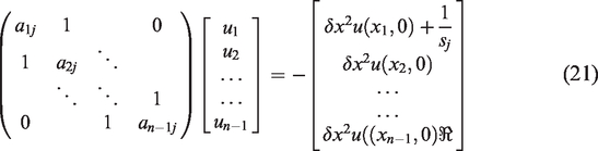
Using a central-difference scheme on the space derivative, the finite difference scheme for (18) is,


The Stehfest algorithm for numerically inverting the Laplace transform
In their wide-ranging study of algorithms for inverting the Laplace transform Davies and Martin 10 cite the Stehfest algorithm [15] as providing accurate results on a wide variety of test functions. Since then this algorithm has become widely used for inverting the Laplace Transform and being favoured due to its reported accuracy and ease of implementation.
The algorithm takes the transformed data in the Laplace space F(s) and produces

The numerical inversion is given by

Theoretically, f(t) becomes more accurate for larger M, but the reality is that rounding errors worsen the results if M becomes too large. According to Stehfest,“The optimum M is approximately proportional to the number of digits the machine is working with”. 11
Also in our earlier work we found that the Stehfest algorithm does not handle noisy data well. 8 As we show in section ‘Numerical examples and discussion’, this can have the effect of introducing perturbations into the travelling wave solutions of the Fisher-KPP equation.
The fixed Talbot algorithm for numerically inverting the Laplace transform
Here we use the function

which maps the closed interval

(See Logan 12 for the details of this transformation).
Next we follow the procedure as adopted by Logan for numerically integrating (27).
With


For convenience we write,


The integral in (30) is then rotated by

Numerical examples and discussion
Example 1
For our first example we use (10)


Ablowitx and Zeppetella
13
give an exact solution for a particular wave speed

When we first implemented the LTFDM it produced distortions in the upper tail of the travelling wave for larger values of t. This is shown in Figure 1. We eventually surmised that these distortions were due to the existence of perturbations of infinite extent. In other words, the approximation of the initial condition on a finite domain. A stability analysis carried out by Gazdang et al. 14 showed that super speed waves or waves with speed greater than Cmin could be maintained if subject only to infinitesimally small positive pertubations.

Profile without time discretisation. t = 1.5.
As is well known, the numerical inversion of the Laplace transform is a perturbed problem. Thus perturbations generated by the numerical scheme itself can then introduce noise into the inversion algorithms which cannot be completely filtered out. However, we found that these perturbations can be reduced if some time discretisation, together with a reinitialisation of the initial condition, is introduced into the numerical method. While the full benefit of using the Laplace transform, i.e., to solve for any time t is partially diminished, introducing some measure of time discretisation meant we were able to use larger time steps than would be the case for other finite difference methods. 15
As we have shown in our previous work,
8
the Fixed Talbot inversion method is more efficient at filtering out this noise than the more widely used Stehfest algorithm. This is shown in Figures 2 and 3 where oscillations in the right-hand tail are present when using the Stehfest inversion method for the time step t = 0.8 but are absent in the Talbot inversion method. Thus smaller time steps are required for comparable accuracy for the Stehfest inversion than for the Talbot. Because of its inability to deal adequately with noisy data, the Stehfest algorithm is also sensitive to the spatial step size δx as smaller space discretisations can also introduce round-off error into our computations. Hence our choice of using the Talbot algorithm for carrying out the LTFDM inversion procedure.

Profile using Stehfest. t = 0.8.

Profile using Talbot. t = 0.8.
The Talbot algorithm is also very effective in dealing with the build-up of round-off error in the right tail of the waves. As Canosa points out “This does not seem due to the numerical method used but to the physical nature of the problem described by the equation which gives rise to an exponential growth of the solutions when this is exponentially small. This basic difficulty makes it difficult to do a rigorous simulation of the solutions of Fisher’s equation”.
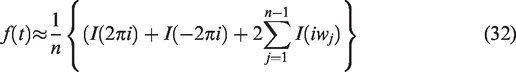
This effect is shown in Figure 4. However, we overcome this problem by merely increasing n in (32) from n = 55 to 555, which completely removes the instability and restores the travelling wave profile Figure 5. The restoration of the travelling profile is due to the Talbot algorithm’s ability to filter out noise with increasing n. 8

Talbot: n = 55 for t = 1 to 5.

Talbot: n = 555 for t = 1 to 5.
While no exact solutions exist for (1) for wave speeds other than

With
Example 2
Cattani, Carlo et al.
17
give an exact solution for the Fisher type equation,


The exact solution is,

Since no exact solution exists for all wave speeds for (36) we derived a perturbation solution to test the numerical scheme at a variety of wave speeds. The perturbation solution for this case is given as,

Results
In our investigations we found our algorithm performs with equal accuracy for space steps
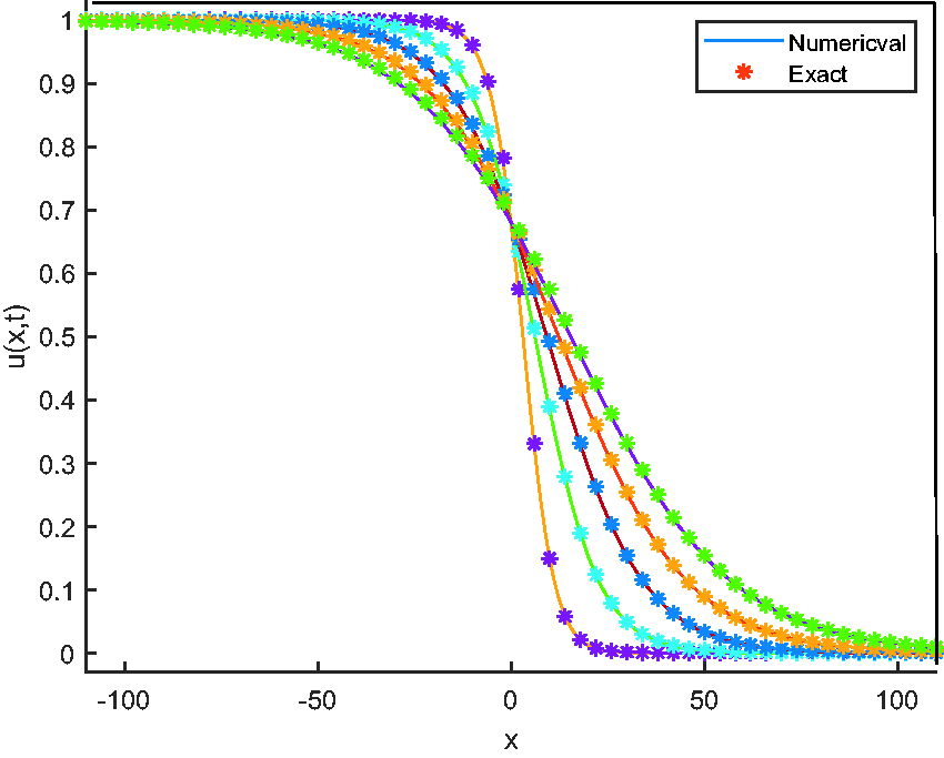
Figure 6 shows the travelling wave profile for (11) example 1, compared with exact solution.
13
The time discretisation used in the LTFDM is

Profile
Figure 7 shows the travelling wave profile for (32) example 2 with exact solution.
17
The time descritisation used in the LTFDM is

Profile
Figure 8 shows the travelling wave profile for example 1 compared with the perturbation solution for wave speeds
Profile Example 1,
Figure 9 shows the travelling wave profile for example 2 compared with perturbation solution (41) for wave speeds
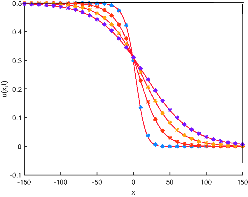
Profile Examole 2,

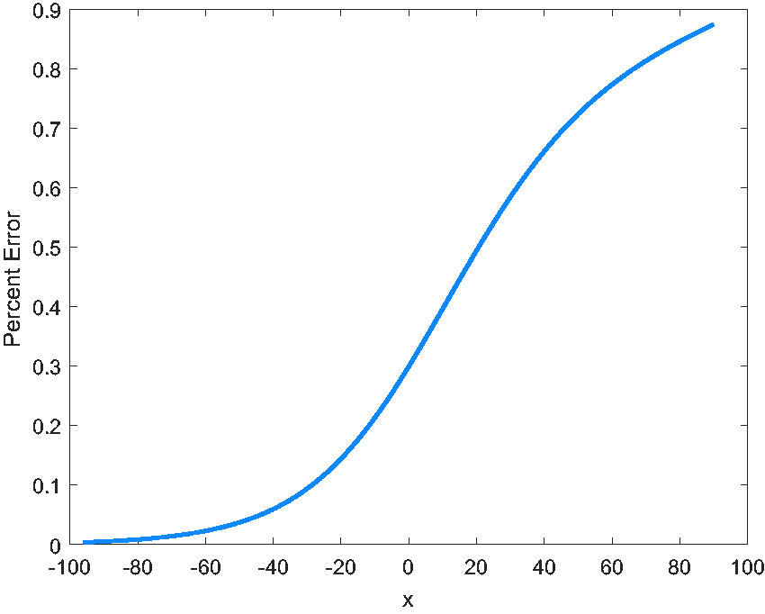
Example 1 Error Profile

Example 1 Error Profile

Example 1 Error Profile
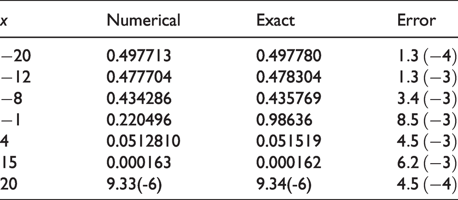
Tables 1-3 present the results for Example 1 for times t = 1, t = 2, and t = 4. For all cases shown we set
Tables 4-6 present the results for problem 2 for times t = 1, t = 2, and t = 4. For all cases shown we set
For brevity we give a sample of the results in Tables 7-9 of the comparison of our method with the approximate perturbation solution for example 2 with t = 1. The length L is increased for higher wave speeds to ensure full propagation of the wave as it moves to the right with increasing speed. In all cases n = 555
Example 2 Error Profile

Example 2 Error Profile

Example 2 Error Profile

Example 2 Error Profile
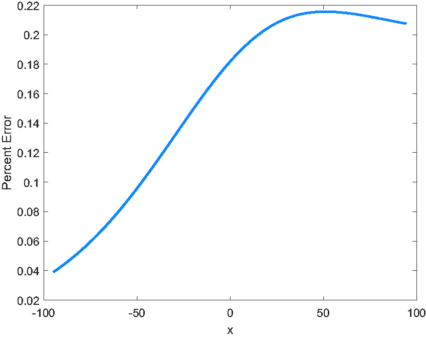
Example 2 Error Profile
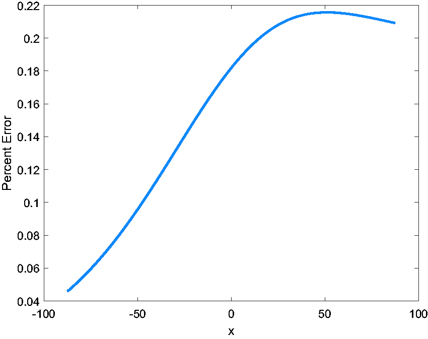
Example 2 Error Profile

Example 2 Error Profile
Example 1, t = 1.

Example 1, t = 2.

Example 1, t = 4.

Example 2. t = 1.
Example 2. t = 2.

Example 2. t = 4.

Example 2 t = 1 C = 10.

Example 2 t = 1 C = 15.

Example 2, t = 1 C = 20.

Conclusion
This paper proposes a numerical approach to the solution of the Fisher-KPP reaction-diffusion equation in which the space variable is developed using a purely finite difference scheme and the time development is obtained using a hybrid Laplace Transform Finite Difference Method (LTFDM). This method to our knowledge has not previously been applied to the Fisher-KPP equation, and Laplace transform methods are generally not deemed suitable for equations which have travelling wave solutions.
However, by introducing some time discretisation into our LTFDM we were able to obtain results which have less than one per cent error over a range of times, space and time discretisation, for variety of wave speeds. The time discretisation was necessary to reduce perturbations of infinite extent which occur in numerical schemes for the Fisher-KPP equation. These perturbations can have a detrimental effect on the LTFDM since all the numerical schemes for inverting the Laplace transform are highly perturbed problems.
Thus crucial to the success of the method outlined in this paper is the choice of the Fixed Talbot inversion algorithm which as we have shown in our earlier work is best at dealing with the inherent noise generated in finite difference schemes. This algorithm also had the effect of ironing out the build-up of round-off error in the right-hand tail of the travelling wave a consequence of the physical nature of the problem.