Sage Journals: Discover world-class research

Abstract

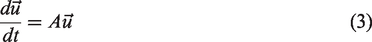
The Weeks method for the numerical inversion of the Laplace transform utilizes a Möbius transformation which is parameterized by two real quantities, σ and b. Proper selection of these parameters depends highly on the Laplace space function F(s) and is generally a nontrivial task. In this paper, a convolutional neural network is trained to determine optimal values for these parameters for the specific case of the matrix exponential. The matrix exponential e^A is estimated by numerically inverting the corresponding resolvent matrix ${(s I - A)}^{- 1}$ via the Weeks method at $(σ, b)$ pairs provided by the network. For illustration, classes of square real matrices of size three to six are studied. For these small matrices, the Cayley-Hamilton theorem and rational approximations can be utilized to obtain values to compare with the results from the network derived estimates. The network learned by minimizing the error of the matrix exponentials from the Weeks method over a large data set spanning $(σ, b)$ pairs. Network training using the Jacobi identity as a metric was found to yield a self-contained approach that does not require a truth matrix exponential for comparison.

Keywords

Numerical Laplace transform inversion Weeks’ method machine learning matrix exponential

Introduction

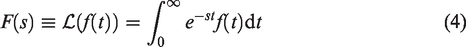
In 1966, while working at IBM, William Weeks presented an algorithm to perform a numerical Laplace transform inversion by expanding in terms of Laguerre polynomials. In his approach, he introduced two real parameters σ and b. He then proceeded to provide a few heuristic rules for determining optimal $(σ, b)$ pairs and illustrated the efficacy of his algorithm for test cases that were numerically tractable at that time. Since then, the Weeks method has become one of a handful of well-known algorithms for numerically inverting a Laplace space function F(s) to the time domain f(t). None-the-less, the problem of optimally selecting the $(σ, b)$ parameters in his algorithm remains difficult for arbitrary functions.

Machine learning is currently quickly evolving into a powerful tool for solving a wide variety of pattern recognition and optimization problems. Convolutional neural networks in particular are now readily available and can be quickly constructed in high level languages such as MATLAB. In previous works, the authors have explored the optimal selection of Weeks’ method parameters by conventional search algorithms and also applied Weeks’ method to the solution of practical engineering problems. Given these experiences and the growth of machine learning, training a neural network to assist with the optimal $(σ, b)$ problem in the Weeks method has therefore seemed like a natural application with real utility.

In this paper, we demonstrate that this machine learning approach can in fact be effective in the Weeks method for numerical inversion of the Laplace transform. To illustrate, we apply the Weeks method to the computation of the matrix exponential. The use of Laplace transform methods for matrix exponentiation is method twelve of the nineteen approaches described in the often cited work by Moler and Van Loan.¹ This follows from the general definition of a complex function $f : M_{n} (ℂ) \to M_{n} (ℂ)$ of a square complex matrix $A \in M_{n} (ℂ)$

f (A) \equiv \frac{1}{2 π i} \int_{Γ} f (s) {(s I - A)}^{- 1} d s

(1)

In the particular case that scalar integrand function $f (s) = e^{s t}$ , one obtains a definition for the matrix exponential

e^{A t} \equiv \frac{1}{2 π i} \int_{Γ} e^{s t} {(s I - A)}^{- 1} d s

(2)

One recognizes from this that the Laplace transform space function corresponding to the matrix exponential $f (t) = e^{A t}$ is the resolvent matrix $F (s) = {(s I - A)}^{- 1}$ . Alternatively, from the perspective of differential equations, the matrix exponential and resolvent matrix are the Laplace transform pair which arise from a set of first order ordinary differential equations involving matrix A and $\vec{u} \in ℂ_{n}$ .²

\frac{d \vec{u}}{d t} = A \vec{u}

(3)

F (s) \equiv L (f (t)) = \int_{0}^{\infty} e^{- s t} f (t) d t

(4)

f (t) \equiv L^{- 1} (F (s)) = \frac{1}{2 π i} \int_{Γ} e^{s t} F (s) d s

(5)

\hat{u} = {(s I - A)}^{- 1} {\vec{u}}_{0}

(6)

\vec{u} (t) = e^{A t} {\vec{u}}_{0}

(7)

The importance of the matrix exponential in the numerical solution of partial differential equations and in numerous practical engineering problems has also motivated its accurate calculation as a focus for this paper.

Our paper is organized into five parts. After this first introductory section, the second part of the paper reviews the Weeks method. Of particular important here are the role of the Möbius transformation and the introduction of the two parameters ( $σ, b)$ . In the third section, we describe the regression neural networks we constructed for predicting optimal $(σ, b)$ values for computing a matrix exponential based on the input matrix. In this section, we also describe how the network was trained on data sets for four classes of matrices and with three different metrics. Algorithms for computing ”truth” values for the matrix exponential based on the Cayley-Hamilton theorem and by rational approximation is also discussed since they are critical to the definition of the three metrics. The fourth section presents the results from the network training and describes the validation process and its results for the four matrix classes. The 3 × 3 skew-symmetric rotation evolution, 4 × 4 quaternion evolution, 5 × 5 random, and 6 × 6 Dramadah matrices used for illustration are also discussed there. The concluding section summarizes the findings and suggests directions for future research.

The Weeks method

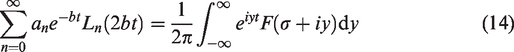
Weeks’ method is one of the most well known algorithms for the numerical inversion of a Laplace space function.^3–6 (The notation in this paper follows the conventions used by Weideman.^7–9 ) A recent survey of numerical inversion algorithms lists the Weeks’ method and three of its variants on the top of this list.¹⁰ It is in part due to its popularity when compared to other inversion algorithms that it has been chosen for this paper. One of the strengths of the Weeks method over other well known approaches, such as the Talbot method,^11–14 the Fourier series method¹⁵ , or Post’s formula^16–18 is that it returns an explicit expression for the time domain function. In particular, Weeks’ method assumes that a smooth function of bounded exponential growth $f (t) : [0, \infty) \to ℂ$ , given by the inverse Laplace transform of a complex function $F (s) : ℂ \to ℂ$

f (t) = \frac{1}{2 π i} \int_{Γ} e^{s t} F (s) d s

(8)

where Γ is a contour in the complex plane, can be expressed as the limit of an expansion in scalar Laguerre polynomials

f (t) = e^{σ t} \sum_{n = 0}^{\infty} a_{n} e^{- b t} L_{n} (2 b t)

(9)

f_{N} (t) \approx e^{σ t} \sum_{n = 0}^{N - 1} a_{n} e^{- b t} L_{n} (2 b t)

(10)

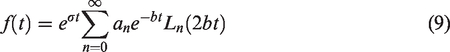
The polynomials $L_{n} (x)$ for $n \geq 0$ are defined by the equation

L_{n} (x) = \frac{e^{x}}{n!} \frac{d^{n}}{d x^{n}} (e^{- x} x^{n})

(11)

x \in (0, \infty)

The coefficients a_n, which may be scalars, vectors, or matrices, contain the information particular to the Laplace space function F(s) and may be complex if f(t) is complex. More importantly, these coefficients are time independent so that f(t) can be evaluated at multiple times from a single set of coefficients.

The two free scaling parameters σ and b in the expansion must be selected according to the constraints that $0 < b$ and $σ_{0} \leq σ$ , where σ₀ is the abscissa of convergence for the singularities of F(s). The restriction of b to positive values ensures that the weighted Laguerre polynomials $e^{- b t} L_{n} (2 b t)$ are well behaved for large t, as shown in Figure 1. This condition also implies that $| e^{- b t} L_{n} (2 b t) | < 1$ . The convergence of the series is uniform.

Figure 1.

Laguerre polynomials $e^{- b t} L_{n} (2 b t)$ .

To compute the coefficients a_n for a general vector or matrix function F(s) one must perform the contour integration in the complex plane of equation (8). If one chooses the Bromwich contour $Γ (s) = σ + i y$ , with $σ_{0} \leq σ$ and y a real number

f (t) = \frac{e^{σ t}}{2 π} \int_{- \infty}^{\infty} e^{iyt} F (σ + i y) d y

(12)

and assumes the expansion

f (t) = e^{σ t} \sum_{n = 0}^{\infty} a_{n} e^{- b t} L_{n} (2 b t)

(13)

then equating the two expressions yields

\sum_{n = 0}^{\infty} a_{n} e^{- b t} L_{n} (2 b t) = \frac{1}{2 π} \int_{- \infty}^{\infty} e^{iyt} F (σ + i y) d y

(14)

Conveniently, the weighted Laguerre polynomials have the Fourier representation⁷

e^{- b t} L_{n} (2 b t) = \frac{1}{2 π} \int_{- \infty}^{\infty} e^{iyt} \frac{{(i y - b)}^{n}}{{(i y + b)}^{n + 1}} d y

(15)

Performing the appropriate substitution, assuming it is possible to interchange the sum and integral, and equating integrands thus leaves

\sum_{n = 0}^{\infty} a_{n} \frac{{(i y - b)}^{n}}{{(i y + b)}^{n + 1}} = F (σ + i y)

(16)

The functions $\frac{{(i y - b)}^{n}}{{(i y + b)}^{n + 1}}$ form a complete, orthogonal basis in $L_{2} (ℝ)$ ⁷

In principle, one could try to use directly the orthogonality of the basis to determine a_n. These functions are highly oscillatory but could possibly be accurately estimated with adaptive integration. Weeks’ insight was however to apply a Möbius transformation.

The Möbius transformation is one of the most fundamental mappings in mathematics.^19–21 Algebraically, it can be expressed as the conformal mapping from the complex plane s to complex plane w according to $w = \frac{A s + B}{C s + D}, (A, B, C, D) \in ℂ$ . The mapping is unique only up to an arbitrary scaling parameter. It is common when utilizing the mapping analytically, but not necessary, to allow the determinant $A D - B C = 1$ . One of the mapping’s properties that is particularly relevant to the current discussion is that it maps circles in s to circles in w. If the Bromwich contour $s = σ + i y$ is viewed as a circle with infinite radius, then its mapping is also a circle. Another relevant property of this transformation is that the singularities of F(s) in the half-plane $σ < σ_{0}$ are mapped to the exterior of the unit circle in the w plane. An exception to this occurs when F(s) has a singularity at infinity which then maps onto the unit circle itself (5) . In the following we will assume that the singularities of F(s) occur in a finite region of the complex plane. The resolvent matrix $F (s) = {(s I - A)}^{- 1}$ Laplace space function corresponding to the matrix exponential e^A clearly belongs to this class of functions.

In his method, Weeks’ choose for the Möbius transformation $(A = 1, B = - σ - b, C = 1, D = - σ + b)$ . The corresponding determinant is then $A D - B C = 2 b$ and

w = \frac{s - σ - b}{s - σ + b}

(17)

For the Bromwich contour $s = σ + i y$

w = \frac{i y - b}{i y + b}

(18)

Using $y = \frac{i b (w + 1)}{w - 1}$ along the Bromwich contour, equation (16) can be expressed as

\sum_{n = 0}^{\infty} a_{n} w^{n} = (i y + b) F (σ + i y)

(19)

\sum_{n = 0}^{\infty} a_{n} w^{n} = \frac{2 b}{1 - w} F (σ - b \frac{w + 1}{w - 1})

(20)

The coefficients a_n of the original expansion (9) are the coefficients of a Maclaurin series. The radius of convergence R is strictly greater than unity due to our selection of functions F(s) which do not have a singularity at infinity. Furthermore, within this radius, the power series converges uniformly.

Cauchy’s integral theorem²² provides a method to compute a_n. Since the function is analytic inside the radius of convergence R > 1, the integration can be performed along the unit circle $w = e^{i θ}$

a_{n} = \frac{1}{2 π i} \int_{| w | = 1} \frac{1}{w^{n + 1}} \frac{2 b}{1 - w} F (σ - b \frac{w + 1}{w - 1}) d w

(21)

a_{n} = \frac{1}{2 π} \int_{- π}^{π} e^{- i n θ} \frac{2 b}{1 - e^{i θ}} F (σ - b \frac{e^{i θ} + 1}{e^{i θ} - 1}) d θ

(22)

Numerically the evaluation of the integral can be computed very accurately using the midpoint rule; $θ_{m} = \frac{m π}{M}$ , where $n = 0, \dots, N - 1$ and $m = - M, \dots, M - 1$

a_{n} \approx \frac{e^{- i n π / (2 M)}}{2 M} \sum_{m = - M}^{M - 1} \frac{2 b e^{- i n θ_{m}}}{1 - e^{i θ_{m + 1 / 2}}} F (σ - b \frac{e^{i θ_{m + 1 / 2}} + 1}{e^{i θ_{m + 1 / 2}} - 1})

(23)

For N = M, this sum can be efficiently computed using the fast Fourier transform⁷ in $O (N log (N))$ operations. The coefficients corresponding to negative indices which result from the FFT algorithm are not needed for the summation and are neglected.

Once the coefficients have been computed and the parameters selected, it is necessary to perform the Laguerre expansion. A naive approach is to generate the Laguerre polynomials using the recurrence relation

(n + 1) L_{n + 1} (x) = (2 n + 1 - x) L_{n} (x) - n L_{n - 1} (x)

(24)

with starting values

L_{0} (x) = 1

L_{1} (x) = 1 - x

multiply by the coefficients, and compute the sum

f (t) = e^{(σ - b) t} \sum_{n = 0}^{\infty} a_{n} L_{n} (2 b t)

(25)

The Laguerre polynomials however can be large for increasing n and thus lead to an unstable summation. A stable method which does not require explicit evaluation of the Laguerre polynomials is the backward Clenshaw algorithm.²³

This brings us now to consider is the effect of the $(σ, b)$ choice on the numerical integration. This is illustrated in Figure 2 where the σ parameter is varied and b held fixed. The truncated contour plotted is $s = σ + i y, | y | \leq 10$ . One clearly sees that varying σ, while holding b = 1/2, yields the exact same discrete mapped points on the unit circle in the w plane. Varying σ in the s plane moves the contour closer to or further away from poles but in the w plane this action translates to leaving the circular contour fixed and moving the mapped poles.

Figure 2.

$z \to w$ mappings with σ varied and b = 1/2.

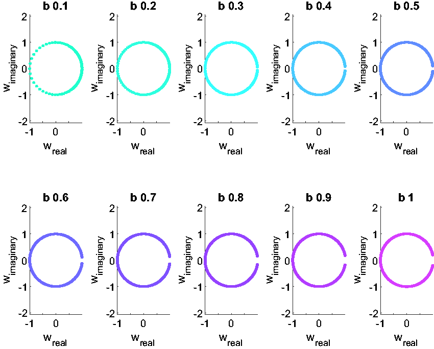
The multifaceted roles that the b parameter plays in the Weeks method is more complex. The parameter can be seen to play at least three roles. One role is that b is a time scaling parameter in the Laguerre polynomial expansion. A second role is that it is 1/2 the determinant in the Möbius transformation. As noted earlier, a Möbius transformation $w = \frac{A z + B}{C z + D}, (A, B, C, D) \in ℂ$ is unique only up to an arbitrary scaling parameter. Given this ambiguity, it is common in analytic computations to define parameters so that the determinant is unity. In the standard Weeks formulation, the determinant is 2 b. Setting b = 1/2 therefore appears natural and indeed in the original 1966 paper by William Weeks, he chooses this value as his starting point before later allowing it to vary in order to accommodate numerical errors given the limited precision available to him at the time.

In the third role, b defines the amount of contour truncation that is acceptable when evaluating the Bromwich integral numerically. Consider the w contours in Figure 3 where the truncated contour $s = σ + i y, | y | \leq 10$ is mapped with σ = 1 and b varying. Typically, when choosing the values for the parameters in the Möbius transformation one picks three mapped pairs of points $(p \to \hat{p}, q \to \hat{q}, r \to \hat{r})$ in the z and w planes and then utilizes the invariance of the cross-ratio under Möbius transformation, equation (26), to arrive at parameters ${A, B, C, D}$ .

\frac{(w - \hat{p}) (\hat{q} - \hat{r})}{(w - \hat{r}) (\hat{q} - \hat{p})} = \frac{(z - p) (q - r)}{(z - r) (q - p)}

(26)

Figure 3.

$z \to w$ mappings with b varied and σ = 1.

In the case of the Weeks method, the three points pairs can be chosen as $z = σ \to w = - 1, z \to + \infty \to w = 1$ , and $z \to - \infty \to w = 1$ . The last two limits can be deduced using L’Hospital’s rule to handle the ratio of infinity values in the Möbius transformation. Clearly, in a numerical integration approach, one cannot map $z = \pm \infty$ and the contour must be truncated. Varying b allows one to adjust the amount.

Machine learning

Neural network

Optimization problems are one of the most important applications of machine learning .^24–27 A currently active of research regarding machine learning is its application to optimal numerical integration.²⁸ While certainly optimization algorithms have been used for parameter selection in numerical Laplace transform algorithms, to our knowledge neural network techniques have not been used previously for optimal parameter selection in the Weeks’ method. In this paper, supervised learning was implemented to train a regression network where the input to the network are the values of the matrix itself and the corresponding continuous output are the $(σ, b)$ pair which provides the most accurate estimate for the matrix exponential from the Weeks method.

To implement the network, we have leveraged the existing capability provided in the MATLAB machine learning toolbox.²⁹ With the basic components provided in the toolbox, we constructed simple convolution neural networks for four classes of matrices. The weights in a network were adjusted to accurately estimate a matrix exponential from the Weeks method with a particular $(σ, b)$ pair.

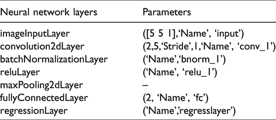
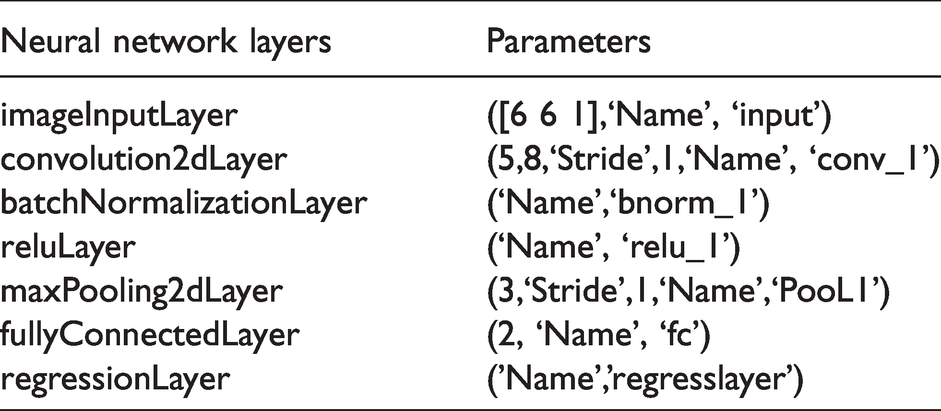
To illustrate, we limited ourselves to square matrices of real values of size 3,4, 5, and 6. A more detailed description of the selected matrices is provided below when describing network training. With respect to the network however, the actual convolutional neural networks used are quite simple. These small matrices allowed for only a few layers such as that shown in Figure 4. The contents on each of the layers is summarized in the Tables 1 to 4 for the four classes of matrices.

Figure 4.

Convolution neural network example.

Table 1.

3 × 3 Direction cosines matrices evolution.

Neural network layers	Parameters
imageInputLayer	([3 3 1],‘Name’, ‘input’)
convolution2dLayer	(2,2,‘Name’, ‘conv_1’)
batchNormalizationLayer	(‘Name’,‘bnorm_1’)
reluLayer	(‘Name’, ‘relu_1’)
maxPooling2dLayer	(2,‘Stride’,2,‘Name’,‘PooL1’)
fullyConnectedLayer	(2, ‘Name’, ‘fc’)
regressionLayer	(‘Name’,‘regresslayer’)

Table 2.

4 × 4 Quaternions evolution.

Neural network layers	Parameters
imageInputLayer	([4 4 1],‘Name’, ‘input’)
convolution2dLayer	(2,2,‘Name’, ‘conv_1’)
batchNormalizationLayer	(‘Name’,‘bnorm_1’)
reluLayer	(‘Name’, ‘relu_1’)
maxPooling2dLayer	(2,‘Stride’,2,‘Name’,‘PooL1’)
fullyConnectedLayer	(2, ‘Name’, ‘fc’)
regressionLayer	(‘Name’,‘regresslayer’)

Table 3.

5 × 5 Random matrices.

Neural network layers	Parameters
imageInputLayer	([5 5 1],‘Name’, ‘input’)
convolution2dLayer	(2,5,‘Stride’,1,‘Name’, ‘conv_1’)
batchNormalizationLayer	(‘Name’,‘bnorm_1’)
reluLayer	(‘Name’, ‘relu_1’)
maxPooling2dLayer	–
fullyConnectedLayer	(2, ‘Name’, ‘fc’)
regressionLayer	(’Name’,’regresslayer’)

Table 4.

6 × 6 Dramadah matrices.

Neural network layers	Parameters
imageInputLayer	([6 6 1],‘Name’, ‘input’)
convolution2dLayer	(5,8,‘Stride’,1,‘Name’, ‘conv_1’)
batchNormalizationLayer	(‘Name’,‘bnorm_1’)
reluLayer	(‘Name’, ‘relu_1’)
maxPooling2dLayer	(3,‘Stride’,1,‘Name’,‘PooL1’)
fullyConnectedLayer	(2, ‘Name’, ‘fc’)
regressionLayer	(’Name’,’regresslayer’)

Detailed descriptions of each of the layers and their available options can be found in the MATLAB toolbox documentation.²⁹ For this specific implementation,the initial layer consists of a MATLAB image layer, where here the ”image” is the matrix A. After this a single convolution layer is applied to the matrix. The results from the convolution are normalized and thresholding is applied. For the activation function, a standard rectified linear unit (ReLu) $f (x) = \max (0, x)$ was utilized. The results are then pooled and flattened down to provide weights for the two outputs $(σ, b)$ . In the final regression layer, the weights are utilized to estimate a $(σ, b)$ pair given the input matrix.

Certainly, a more sophisticated analysis could be performed to develop more accurate neural networks for this application. We choose simple networks in order to illustrate the approach and settled on those shown after some experimentation.

Regarding network training, a summary of the options used can be found in Table 5. The validation and training data are a 5% and 95% fraction of the total database created, respectively.

Table 5.

Network training options.

Matrix	3 × 3	4 × 4	5 × 5	6 × 6
Algorithm	sgdm	sgdm	sgdm	sgdm
MiniBatchSize	128	128	16	16
GradientThreshold	5	5	5	5
InitialLearnRate	0.0005	0.0005	0.0005	0.0005
LearnRateSchedule	piecewise	piecewise	piecewise	piecewise
LearnRateDropPeriod	1	1	1	1
MaxEpochs	5	5	5	5
Verbose	true	true	true	true
Plots	training-progress	training-progress	training-progress	training-progress
Shuffle	every-epoch	every-epoch	every-epoch	every-epoch
ExecutionEnvironment	gpu	gpu	gpu	gpu
ValidationPatience	50	50	50	50
Momentum	0.5	0.5	0.5	0.5
ValidationData	X,Y	X,Y	X,Y	X,Y

Training metrics

To gauge accuracy and to train the network, we considered three different metrics:

Jacobi Identity:

$| \det (e^{A}) - e^{trace (A)} |$

Max Element Error:

$\max_{m, n} | {(e_{m, n}^{A})}_{Weeks} - {(e_{m, n}^{A})}_{truth} |$

Total Elements Error:

$\sum_{m, n} | {(e_{m, n}^{A})}_{Weeks} - {(e_{m, n}^{A})}_{truth} |$

The Jacobi identity metric is particularly interesting in that it provides a self-contained error estimate that depends only on the original matrix A and its approximation e^A. There is no need for another approximation method to utilize for validation.

For the other two metrics based on comparing the Weeks estimated matrix exponential with a truth value, it was necessary to obtain ”truth”. Clearly, utilizing another trusted approximation method and simply comparing approximations is straight forward and is in-fact the approach we have utilized in past publications.^13,30,31 When dealing with two high accuracy methods however, this direct comparison of the two approximations leaves one questioning which of the two is actually the more accurate and thus leads to some ambiguity in the error metric. In this paper, to avoid that ambiguity, we have a employed a 2-out-of-3 error estimate approach. For the max element and total elements error metrics, we have computed the matrix exponential via three different algorithms^1,32–34

Weeks Method

Padé Rational Approximation

Cayley-Hamilton Theorem

The max element and total elements errors are then defined as the minimum of the differences between the Weeks and the Padé approximations and the differences between the Weeks approximation and the Cayley-Hamilton expression.

Error (e_{Weeks}^{A}) =

(27)

\min (δ (e_{Weeks}^{A} - e_{Pade}^{A}), δ (e_{Weeks}^{A} - e_{Cayley - Hamilton}^{A}))

It is assumed that if two of the algorithms agree up to n decimal digits that those digits arose because the algorithms agree up to that accuracy and not due to round-off.

The Padé rational approximation is the algorithm implemented for the matrix exponential in MATLAB’s expm function.³⁵ Briefly, the original matrix is scaled by a factor of $2^{n}$ to create a matrix whose eigenvalues are reduced so that the infinity norm is less than 1/2. A rational approximation is then computed from the reduced matrix. To regain the exponential of the original matrix, the corresponding reduced matrix exponential is squared n times. Written concisely with matrix polynomials P and Q

e^{A} = {(e^{A / 2^{n}})}^{2^{n}} \approx {(\frac{P_{m} (A / 2^{n})}{Q_{m} (A / 2^{n})})}^{2 n}

(28)

The Padé rational approximation approach has the advantages of possessing a well understood error estimate and widespread use due to its inclusion in MATLAB.

For a small square matrix it is not necessary to approximate the matrix exponential as it can be expressed analytically via the Cayley-Hamilton theorem.³⁴ The theorem states simply that every matrix satisfies its own characteristic equation. That is, given a square matrix A with dimension n and with a characteristic polynomial

△ (s) = | s I - A | = s^{n} + c_{n - 1} s^{n - 1} + \dots + c_{o}

(29)

and defining a corresponding matrix polynomial, formed by substituting A for s

△ (A) = A^{n} + c_{n - 1} A^{n - 1} + \dots + c_{o} I

(30)

one has

△ (A) = [0]

A consequence of this theorem, is that the analytic function of a matrix A of dimension n may be expressed as a polynomial of degree (n-1) or less.

f (A) = \sum_{k = 0}^{n - 1} α_{k} A^{k}

(31)

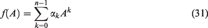
The exponential function is analytic and thus the matrix exponential can be determined by finding expressions for the coefficients 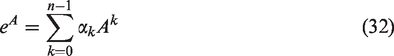${α_{k}}$ .

e^{A} = \sum_{k = 0}^{n - 1} α_{k} A^{k}

(32)

To find those coefficients, it is sufficient to solve the corresponding set of equations given by the eigenvalues of A. For distinct eigenvalues, the eigenvalue equation is

e^{λ_{i}} = \sum_{k = 0}^{n - 1} α_{k} λ_{i}^{k}

(33)

For any eigenvalue of multiplicity m, the first $(m - 1)$ derivatives of $△ (s)$ all vanish at those eigenvalues. In that case, the derivatives up to the multiplicity of the eigenvalue are considered.

f (λ_{i}) = \sum_{k = 0}^{n - 1} α_{k} λ_{i}^{k} = R (λ_{i})

(34)

\frac{d f}{d λ} |_{λ = λ_{i}} = \frac{d R}{d λ} |_{λ = λ_{i}}

(35)

\frac{d^{m - 1} f}{d λ^{m - 1}} |_{λ = λ_{i}} = \frac{d^{m - 1} R}{d λ^{m - 1}} |_{λ = λ_{i}}

(36)

The main disadvantages of the Cayley-Hamilton expressions are the complexity of the analytic expressions and their sensitivity to round-off error. Except for 2 × 2, 3 × 3, and 4 × 4 matrices, analytic expressions for eigenvalues are generally impossible to derive. For our training purposes, however, the formula is tractable and to solve the equations we have used Mathematica (2019).³⁶ Since the Cayley-Hamilton matrix exponential expressions in MATLAB are not easily obtained and they are central to our analysis, we have included for the reader the exact Mathematica script used for solving the equations and their conversion to MATLAB in the supplemental material.³⁷ We also present the specific case of the Cayley-Hamilton theorem applied to a 4 × 4 matrix.

Briefly, for a general square 4 × 4 matrix, there are five eigenvalue cases to consider

All distinct: $λ_{1} \neq λ_{2} \neq λ_{3} \neq λ_{4}$

One pair, other 2 distinct: $λ_{1} \neq λ_{2} \neq λ_{3}, λ_{3} = λ_{4}$

Two distinct pairs: $λ_{1} = λ_{2}, λ_{3} = λ_{4}, λ_{1} \neq λ_{3}$

3 identical, 1 unique: $λ_{1} = λ_{2} = λ_{3}, λ_{1} \neq λ_{4}$

All identical: $λ_{1} = λ_{2} = λ_{3} = λ_{4}$

If we allow $b_{i} = e^{λ_{i}}$ , then the equations to solve in the five cases become:

All distinct

b_{1} = a_{0} + a_{1} λ_{1} + a_{2} λ_{1}^{2} + a_{3} λ_{1}^{3}

(37)

b_{2} = a_{0} + a_{1} λ_{2} + a_{2} λ_{2}^{2} + a_{3} λ_{2}^{3}

(38)

b_{3} = a_{0} + a_{1} λ_{3} + a_{2} λ_{3}^{2} + a_{3} λ_{3}^{3}

(39)

b_{4} = a_{0} + a_{1} λ_{4} + a_{2} λ_{4}^{2} + a_{3} λ_{4}^{3}

(40)

One pair, other 2 distinct

b_{1} = a_{0} + a_{1} λ_{1} + a_{2} λ_{1}^{2} + a_{3} λ_{1}^{3}

(41)

b_{2} = a_{0} + a_{1} λ_{2} + a_{2} λ_{2}^{2} + a_{3} λ_{2}^{3}

(42)

b_{3} = a_{0} + a_{1} λ_{3} + a_{2} λ_{3}^{2} + a_{3} λ_{3}^{3}

(43)

λ_{3} b_{3} = a_{1} + 2 \cdot a_{2} λ 3 + 3 \cdot a_{3} λ_{3}^{2}

(44)

Two distinct pairs

b_{1} = a_{0} + a_{1} λ_{1} + a_{2} λ_{1}^{2} + a_{3} λ_{1}^{3}

(45)

λ_{1} b_{1} = a_{1} + 2 \cdot a_{2} λ_{1} + 3 \cdot a_{3} λ_{1}^{2}

(46)

b_{3} = a_{0} + a_{1} λ_{3} + a_{2} λ_{3}^{2} + a_{3} λ_{3}^{3}

(47)

λ_{3} b_{3} = a_{1} + 2 \cdot a_{2} λ_{3} + 3 \cdot a_{3} λ_{3}^{2}

(48)

3 identical, 1 unique

b_{1} = a_{0} + a_{1} λ_{1} + a_{2} λ_{1}^{2} + a_{3} λ_{1}^{3}

(49)

λ_{1} b_{1} = a_{1} + 2 \cdot a_{2} λ_{1} + 3 \cdot a_{3} λ_{1}^{2}

(50)

λ_{1}^{2} \cdot b_{1} = 2 \cdot a_{2} + 6 \cdot a_{3} λ_{1}

(51)

b_{4} = a_{0} + a_{1} λ_{4} + a_{2} λ 4^{2} + a_{3} λ_{4}^{3}

(52)

All identical

b = a_{0} + a_{1} λ + a_{2} λ^{2} + a_{3} λ^{3}

(53)

λ b = a_{1} + 2 \cdot a_{2} λ + 3 \cdot a_{3} λ^{2}

(54)

λ^{2} \cdot b = 2 \cdot a_{2} + 6 \cdot a_{3} λ

(55)

λ^{3} \cdot b = 6 \cdot a_{3}

(56)

A simple check of these equations is to note for the case that all of the eigenvalues are identical, the coefficients are simply

a_{3} = (1 / 6) b λ^{3}

(57)

a_{2} = (1 / 2) b λ^{2} \cdot (λ^{2} - 1)

(58)

a_{1} = b λ (1 + λ^{2} - (4 / 3) λ^{4})

(59)

a_{0} = b (1 + (2 / 3) λ^{6} - (1 / 2) λ^{4} - λ^{2})

(60)

If the matrix is the 4 × 4 identity matrix, then $e^{I} = e \cdot I$ , λ = 1, $b = e^{1}$ , and the coefficient equations simplify to

a_{3} = e / 6

(61)

a_{2} = 0

(62)

a_{1} = (2 / 3) e

(63)

a_{0} = (1 / 6) e

(64)

Now performing the sum (32), $e^{I} = (1 / 6) e I + (2 / 3) e I + 0 * I^{2} + (1 / 6) * I^{3}$ or $e^{I} = e (1 / 6 + 2 / 3 + 1 / 6) I = e \cdot I$ , which confirms our calculations.

Test case matrices

To illustrate the formalism outlined above, we have computed the matrix exponential of four square matrices

3 × 3 Skew Symmetric Direct Cosine Matrix Evolution Matrices

4 × 4 Quaternion Evolution Matrices

5 × 5 Random Correlation Matrices

6 × 6 Dramadah Matrices

The 3 × 3 and 4 × 4 skew symmetric and quaternion evolution matrices are those in the ordinary differential equations that describing rigid body rotation.^38,39 For a 3 × 3 direction cosines matrix (DCM) M, its evolution in the absence of external forces is described by a cross product of the rotation rates vector with the DCM. This cross-product can be expressed as a skew symmetric 3 × 3 matrix A.

\frac{d M}{d t} = A \cdot M

(65)

A = (\begin{matrix} 0 & - ω_{ψ} & ω_{θ} \\ ω_{ψ} & 0 & - ω_{ϕ} \\ - ω_{θ} & ω_{ϕ} & 0 \end{matrix})

(66)

Since the 3 × 3 matrix is real and skew-symmetric it has eigenvalues which are are either zero or purely imaginary, specifically $λ_{1} = 0, λ_{2, 3} = \pm i \sqrt{ω_{ψ}^{2} + ω_{θ}^{2} + ω_{ϕ}^{2}}$ .

The case is similar for the 4-vector of quaternions $\vec{q}$

\begin{array}{l} \vec{q} = [\begin{matrix} \cos (δ) \\ \cos (α) \sin (δ) \\ \cos (β) \sin (δ) \\ \cos (γ) \sin (δ) \end{matrix}] \\ α, β, γ = direction angles o f the axis \\ δ = measure o f rotation angle \\ \hat{u} = {\cos (α), \cos (β), \cos (γ)} \\ = unit vector axis o f rotation \end{array}

(67)

One can define an ordinary differential equation for the evolution of $\vec{q}$ by means of a real skew symmetric matrix

\frac{d \vec{q}}{d t} = A \cdot \vec{q}

(68)

A = \frac{1}{2} (\begin{matrix} 0 & - ω_{1} & - ω_{2} & - ω_{3} \\ ω_{1} & 0 & ω_{3} & - ω_{2} \\ ω_{2} & - ω_{3} & 0 & ω_{1} \\ ω_{3} & ω_{2} & - ω_{1} & 0 \end{matrix})

(69)

This choice for $\vec{q}$ and the matrix A is only one of a number of possible formulations.³⁹ The solution to this equation is however also the matrix exponential $\vec{q} (t) = e^{A t} {\vec{q}}_{0}$ and the eigenvalues are either zero or purely imaginary. Specifically, $λ_{1, 2} = \frac{i}{2} \sqrt{ω_{1}^{2} + ω_{2}^{2} + ω_{3}^{2}}$ and $λ_{3, 4} = - \frac{i}{2} \sqrt{ω_{1}^{2} + ω_{2}^{2} + ω_{3}^{2}}$ .

For 5 × 5 matrices, real square 5 × 5 random correlation matrices were selected. The matrices were chosen to stress the neural network approach studied here. We have also studied the matrix exponential of random matrices to some extent in our previous publication,¹³ which utilized a Dempster-Shafer evidential theory approach to parameter selection in Talbot’s method for numerical inversion, and thus it seemed appropriate to do so again here. To create the database, we leveraged the MATLAB gallery matrix function gallery(’randcorr’,n) with n = 5. This generates a random square correlation matrix that is symmetric positive semidefinite with ones on the diagonal. The eigenvalues from these matrices are real, drawn from a uniform distribution, and thus are distributed fundamentally differently in the complex plane than for the 3 × 3 and 4 × 4 rotation matrices.

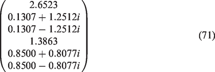
The 6 × 6 Dramadah matrix is the largest matrix for which we computed the matrix exponential using the Weeks, Padé, and Cayley-Hamilton methods. This matrix was also constructed by leveraging the MATLAB gallery matrix gallery(’dramadah’,6,3). This is a binary matrix (70) of zeros and ones.

(\begin{matrix} 1 & 1 & 0 & 0 & 0 & 0 \\ 0 & 1 & 1 & 0 & 0 & 0 \\ 1 & 0 & 1 & 1 & 0 & 0 \\ 0 & 1 & 0 & 1 & 1 & 0 \\ 1 & 0 & 1 & 0 & 1 & 1 \\ 0 & 1 & 0 & 1 & 0 & 1 \end{matrix})

(70)

An interesting fact is that the determinant of the nth Dramadah matrix is the nth Fibonacci number, in this case 8. This can be verified directly from the product of the eigenvalues, which are approximately equal to:

(\begin{matrix} 2.6523 \\ 0.1307 + 1.2512 i \\ 0.1307 - 1.2512 i \\ 1.3863 \\ 0.8500 + 0.8077 i \\ 0.8500 - 0.8077 i \end{matrix})

(71)

To vary the values of the Dramadah matrix, the matrix was multiplied by random values from $γ \in [- 1, 1] ∖ 0$ . The eigenvalues of the scaled Dramadah matrices are then clearly scalar multiples of the eigenvalues (71). More importantly, the corresponding inverse matrix becomes $(1 / γ) A^{- 1}$ where

A^{- 1} = (\begin{matrix} 5 & - 3 & 2 & - 1 & 1 & - 1 \\ 3 & 3 & - 2 & 1 & - 1 & 1 \\ - 3 & 5 & 2 & - 1 & 1 & - 1 \\ - 2 & - 2 & 4 & 2 & - 2 & 2 \\ - 1 & - 1 & - 2 & 5 & 3 & - 3 \\ - 1 & - 1 & - 2 & - 3 & 3 & 5 \end{matrix}) / 8

(72)

Given that $| γ | < 1$ , the corresponding inverse matrix may have large values. This could be a challenge for the Weeks method which requires matrix inversion along the integration contour and thus is an excellent stressing case.

Results

With the Weeks method and machine learning approaches outlined above, results from their application are reported here. Two separate sets of results are discussed. First are the results of the supervised training to construct the twelve neural networks, four tests case with the three metrics. The main takeaway from this section is that the simple networks employed were able to capture the shape of the error surface as a function of $(σ, b)$ . The total element and maximum element metrics, as expected, were found to be useful for this purpose. What was surprising and particularly useful to find is that the supervised learning by the neural network with the Jacobi identity led to a predictive network.

The second set of results focus on validation. In particular, we have focused on the neural networks created using the Jacobi identity. The networks based on the other two metrics work very well, but because they require a second approximation for training, we decided to focus on the metric which leads to a self-contained algorithm. Even for the simple neural networks, the validation results demonstrate that machine learning can be utilized with the Weeks method to accurately compute the matrix exponential.

Neural network training results

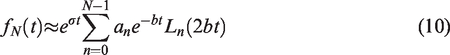
Table 6 contains a summary of the specific set parameters chosen to construct the databases of matrices used to train the networks. In all cases, sixteen Laguerre polynomials were used in the estimate of the matrix exponential. Clearly, accuracy will be dependent on the number of basis functions but for illustration purposes, this number of polynomials was found to be sufficient.

Table 6.

Training database resolution parameters.

Parameter	3 × 3	4 × 4	5 × 5	6 × 6
σ	[0,10]	[0,10]	[0,10]	[0,10]
b	(0,5]	(0,5]	(0,5]	(0,5]
$N_{σ}$	21	21	21	41
$N_{β}$	21	21	21	41

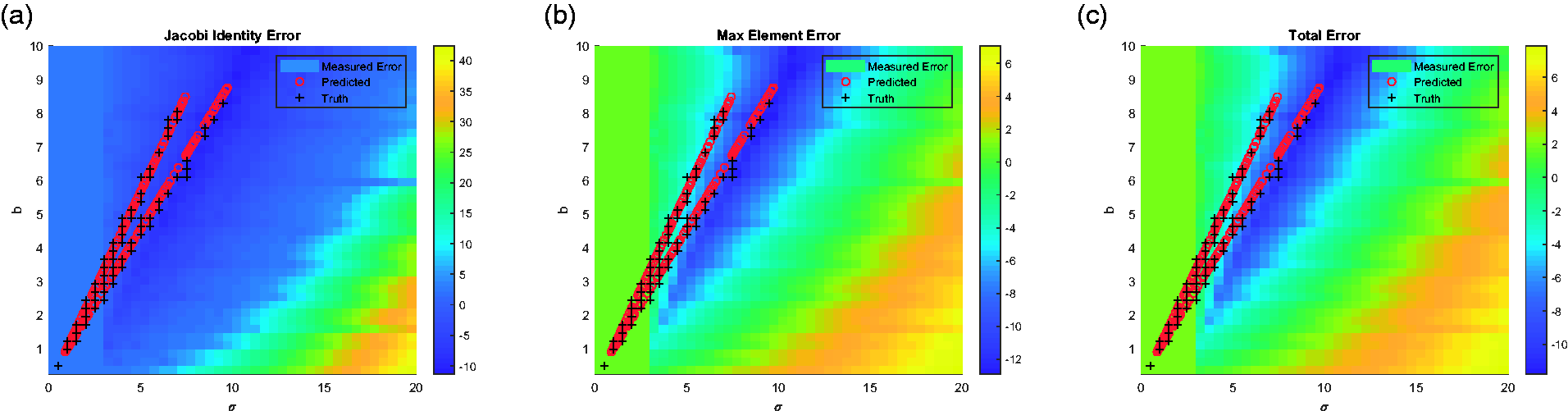
For the 3 × 3 DCM evolution and 4 × 4 quaternion evolution matrices, the matrices were constructed from the angles rates. The roll and yaw rates were taken from dividing the interval $[- 1, 1]$ evenly into 81 intervals, while the pitch was sampled from 41 linearly space intervals from $[- 1, 1]$ . The elements of the random 5 × 5 matrices were those obtained from the MATLAB toolbox directly and drawn from $[- 1, 1]$ . Last, the 6 × 6 Dramadah matrices were formed from multiplying the matrix by a constant values from [–1,1] where values were linearly spaced by 5000 points, excluding 0.

To illustrate the results from the training phase, two types of plots have been constructed. The first is a set of surface plots for error of the Weeks method estimated matrix exponential as a function of $(σ, b)$ as measured by the Jacobi identity metric, the maximum element error metric, and total matrix elements error metric. Recall from the previous discussion, that the truth when creating the element error surfaces is defined based on 2-out-of-3 rule where the Weeks estimate is compared with the Padé and Cayley-Hamilton theorem derived matrix exponentials. The Jacobi identity surface is defined by directly comparing A and the Weeks method estimated matrix exponential. The surfaces plotted are for a typical matrix from each of the four families of matrices, the skew-symmetric (Figure 5), the quaternions (Figure 7), the random (Figure 9), and the Dramadah (Figure 11). For every matrix in each class, we have computed a corresponding surface.

Figure 5.

Error surfaces: 3 × 3 skew symmetric. (a) Jacobi. (b) Max element. (c) Total.

What one finds from these surface plots is that there are general structures to the error surfaces for each of the three metrics. It is therefore possible to find a minimum that corresponds to an optimal $(σ, b)$ for the construction of the matrix exponential for all three metrics.

Also plotted on these surfaces are cross and circle pairs from each of the 5% of validation matrices reserved from the total set of matrices utilized in the process of training the neural network. The crosses mark the $(σ, b)$ pairs that corresponds to the true minimum of the error surfaces for each tested matrix. The circles correspond to the neural network estimated $(σ, b)$ pairs. The cross and circle pairs should be close but are rarely identical due to the finite sampling of the σ and b when creating the surfaces and the fact that the regression from the neural network returns a value on a continous interval. To be clear, the shaded surface is for only one matrix from the class while the crosses and circles are for all of the matrices in the 5% of the data set not used when training the network. For illustration purposes, all of the pairs are shown on the same plot. These figures never-the-less show that there is a pattern to the predictions of the neural network that overlaps with the underlying minimal error surfaces across matrices of a class.

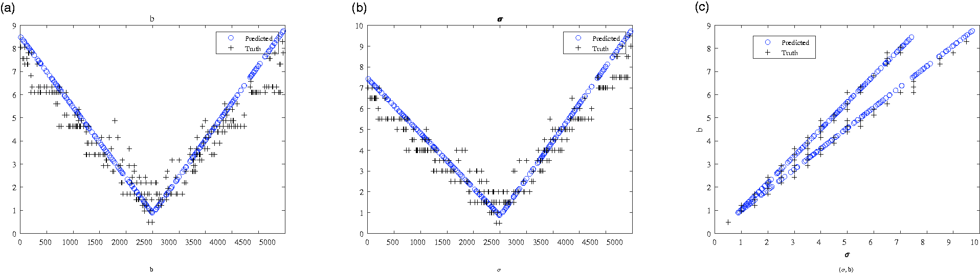
The second set of plots further illustrates that there is a pattern to the predictions of the neural network that overlaps with the underlying minimal error surfaces across matrices of a class. Plotted in Figure 6 for the DCM evolution, Figure 8 for the quaternions, Figure 10 for the random, and Figure 12 for the Dramadah, are the truth and neural network estimated σ and b parameters as a function of the test case. 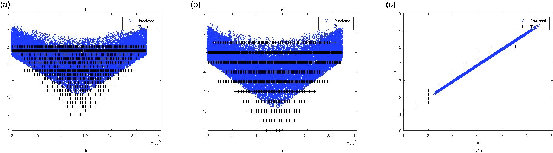These too show that the simple neural networks used for this analysis none-the-less capture the distribution of optimal $(σ, b)$ values as the corresponding matrices are varied.

Figure 6.

Truth vs. prediction: 3 × 3 skew symmetric.

Figure 7.

Error Surfaces: 4 × 4 quaternions. (a) Jacobi. (b) Max element. (c) Total.

Figure 8.

Truth vs. Prediction: 4 × 4 quaternions.

Figure 9.

Error surfaces: 5 × 5 random. (a) Jacobi. (b) Max element. (c) Total.

Figure 10.

Truth vs. prediction: 5 × 5 random.

Figure 11.

Error surfaces: 6 × 6 Dramadah. (a) Jacobi. (b) Max element. (c) Total.

Figure 12.

Truth vs. prediction: 6 × 6 Dramadah.

Validation

In the previous training results, the optimal $(σ, b)$ predictions from the twelve simple neural networks were found to be reasonably accurate when compared to the true minimum on the $(σ, b)$ grid defined in Table 6. For a more extensive validation of the convolutional networks generated to predict Weeks’ method $(σ, b)$ , we here take the full database and both utilize the network to predict a $(σ, b)$ pair and then also demonstrate that the matrix exponential with the Weeks method is reasonably accurate. That is, for every matrix of a class in the database, the corresponding network trained using the Jacobi identity was run to generate an estimated optimal $(σ, b)$ and the error measured. Note that this is different from the training. In the training, all twelve networks were generated and compared on the limited data subset. Here we still use the three error metrics and define the maximum element and total element errors with the 2-out-of-3 rules against the Padé and Cayley-Hamilton estimated exponentials. However, the predictions are solely from the networks trained using the Jacobi identity. We have limited ourselves to only predictions based on the four networks for each class that were trained using the Jacobi identity for the main reason that networks trained using the 2-out-of-3 rule work well but are more difficult to use in practice. When solving differential equations involving much larger matrices, the 2-out-of-3 approach based on the Cayley-Hamilton theorem requires solving systems of equations which become too cumbersome to practically solve. Comparison’s to Padé approximations are reasonable for large matrices, but then one returns to the problem of comparing only two approximations. In contrast, the self-contained Jacobi identity metric is practically feasible for very large matrices.

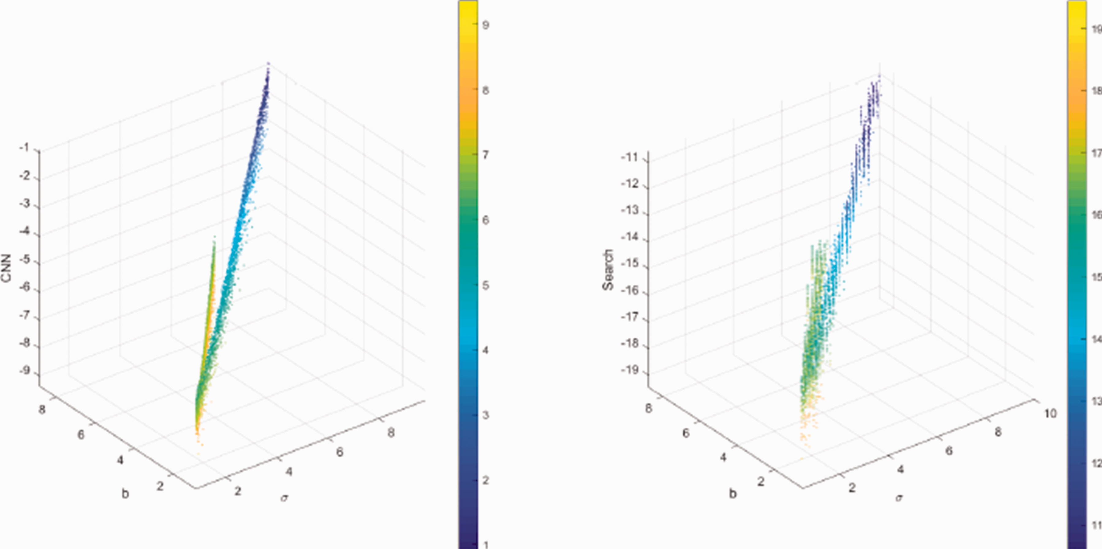
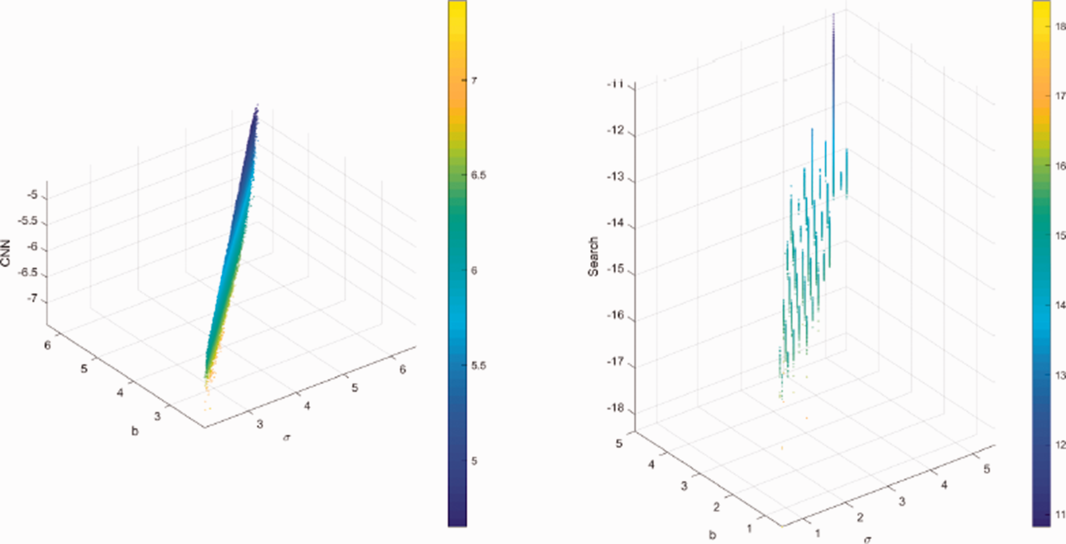
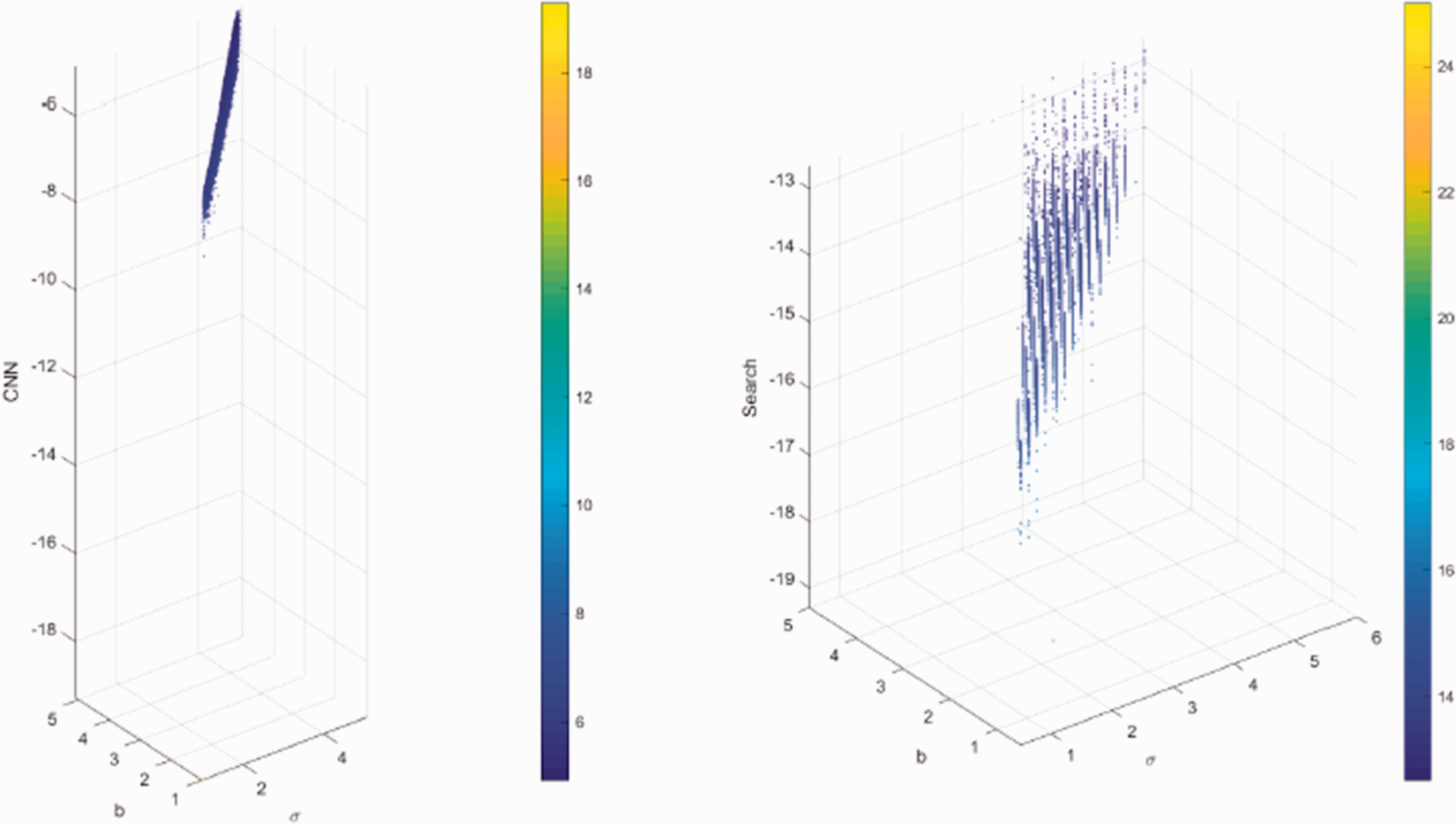
What one observes in the following figures is that while they disagree in the exact amount of error, all demonstrate that the approach outlined in this paper is feasible. Specifically, the error as measured with respect to the Jacobi identity can be found in Figures 13 to 16 for the 3,4,5,and 6 square matrices, respectively. The plots are in log base 10 with the left side being the error based on the network $(σ, b)$ and the right side being the actual minimum error from any $(σ, b)$ sampled when creating the database. Each point in the figures corresponds to a matrix in the complete database. One finds from investigating this figures that the slow full scale minimization of the Jacobi error surface yields excellent results for the Weeks estimated matrix exponential. The neural network derived values, being much faster, are bounded $10^{- 6}$ for the 3 × 3 and 4 × 4 matrices. For the 5 × 5 and 6 × 6, the Jacobi errors of the Weeks method estimated exponentials with the simple networks are higher but still follow the correct distribution.

Figure 13.

Jacobi error: 3 × 3 skew symmetric matrix.

Figure 14.

Jacobi error: 4 × 4 quaternions evolution matrix.

Figure 15.

Jacobi error: 5 × 5 random matrix.

Figure 16.

Jacobi error: 6 × 6 Dramadah.

The maximum per element matrix error results are plotted in Figures 17 to 20 for the four matrix families. Finally, those based on the total element error are found in Figures 21 to 24. The points across the three metric plots are for the same matrix exponential estimates. The maximum element and total element error calculations also provide a clear picture that the simple neural networks have been able to reasonably capture the basic minimum error surface shape for the four classes.

Figure 17.

Max element error: 3 × 3 skew symmetric matrix.

Figure 18.

Max element error: 4 × 4 quaternions evolution matrix.

Figure 19.

Max element error: 5 × 5 random matrix.

Figure 20.

Max element error: 6 × 6 Dramadah.

Figure 21.

Total elements error: 3 × 3 skew symmetric matrix.

Figure 22.

Total elements error: 4 × 4 quaternions evolution matrix.

Figure 23.

Total elements error: 5 × 5 random matrix.

Figure 24.

Total elements error: 6 × 6 Dramadah.

As a final summary note on the validation results, in Figures 25 and 26 are the 95% confidence intervals for the error metrics recorded in the previous validation figures. That is, the means and confidence intervals are of the matrix exponential error from the neural network predicted parameters and the direct minimization. From these figures one sees that the neural network based approach does yield similar confidence intervals relative to the mean error as observed from the full minimization. Another interesting result seen is that the Jacobi error metric has considerably wider confidence intervals for the larger matrices than for the smaller two matrices. Given that the Jacobi metric has potentially broader utility for larger matrices than the other two metrics, this fact about the confidence intervals may be of importance in practical applications or for training a network with larger matrices.

Figure 25.

Confidence intervals for network derived errors.

Figure 26.

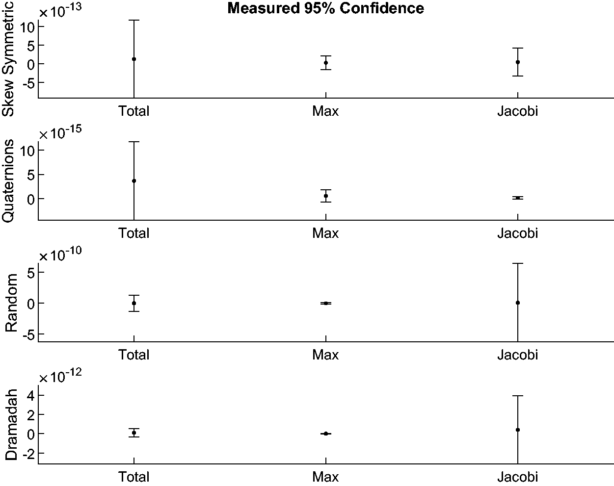
Confidence intervals for measured errors.

Conclusion

In this paper, we have introduced a machine learning based approach to the problem of selecting optimal parameters in Weeks method for the numerical inversion of the Laplace transform. Specifically, we have demonstrated that it is possible to train a convolutional neural regression network to estimate a $(σ, b)$ pair of parameters which yields an accurate numerical inversion when utilized in Weeks’ method. Both the mathematical framework for the approach and concrete results have been presented.

To illustrate, we have focused on the estimation of the matrix exponential e^A by numerically inverting the corresponding resolvent matrix ${(s I - A)}^{- 1}$ . Four classes of matrices were studied, the 3 × 3 skew-symmetric direction cosines evolution matrices, 4 × 4 quaternion evolution matrices, 5 × 5 random matrices, and 6 × 6 Dramadah matrices. For the training and to quantitatively describe the error of the Weeks method estimated matrix exponentials, we considered three metrics. These are the Jacobi identity, a comparison of the maximum per element error, and a comparison of total elements’ error. For the last two metrics, it was necessary to define ”truth” matrix exponentials based on the Padé rational approximation and from the Cayley-Hamilton theorem.

A particularly useful result which came out of this analysis is the ability to train the Weeks method for the matrix exponential directly from the Jacobi identity. Practically speaking, this allows one to potentially train a neural network with the Weeks method for the exponential of matrices of any size without the need for comparison with a truth value. The small matrices used in this study were chosen to illustrate the approach and because it is relatively straightforward to compute their exponentials via the Cayley-Hamilton formula. Moreover, with the rational Padé approximations and the Cayley-Hamilton expressions for these small matrices, it has been possible to accurately estimate the matrix exponential from the Weeks method as the Möbius transformation parameters $(σ, b)$ were discretized. For many applications, particularly those involving partial differential equations, the matrices are much larger and yet their exponentials could be computed with the approach presented in this paper.

For future mathematical research, three avenues are suggested. One is a more thorough investigation into different machine learning techniques for Weeks’ method optimization. The simple convolutional neural networks presented here demonstrate the efficacy of the approach but the choice of network layers and layer options was not fully optimized. There is a rich diversity of neural network architectures which may be more effective than those utilized here.

A second avenue is to reduce the parameters to only σ and allow b to be fixed. This would simplify the neural network training considerably. To compensate for a fixed b parameter, it may be possible to utilize adaptive integration for the numerical quadrature along the Möbius transform mapped unit circle contour in w. With adaptive quadrature, one might be able to outperform the trapezoidal rule approach used in this paper.⁴⁰

Expanding this approach to other Laplace transform pairs is an obvious third avenue for future work. The accurate solution of the differential equations describing viscoelastic beams,⁴¹ the modeling of fluids,⁴² and the high accuracy propagation of electromagnetic waves ¹⁸ are only a few specific examples of difficult problems which may benefit from the machine learning based approach to the Weeks method.

Supplemental Material

sj-zip-1-act-10.1177_1748302621999621 - Supplemental material for Optimal parameter selection in Weeks’ method for numerical Laplace transform inversion based on machine learning

Supplemental material, sj-zip-1-act-10.1177_1748302621999621 for Optimal parameter selection in Weeks’ method for numerical Laplace transform inversion based on machine learning by Patrick O Kano, Moysey Brio and Jacob Bailey in Journal of Algorithms and Computational Technology

Footnotes

Acknowledgements

This paper would not have been possible without the support from a number of colleagues at Raytheon Missile Systems. The authors especially wish to thank Michael Stinely who has been encouraging from the earliest conceptual phases of this work. Also to thank for their support are Nitesh Shah, Chanon Stewart, and Ross Newton. Ultimately, preparing this paper has required time and understanding from family. P. Kano particularly wishes to thank his son Brennan who challenges him with interesting discussions. The idea to explore the application of the approach in this paper to quaternions arose from one such conversation.

Declaration of Conflicting Interests

The author(s) declared no potential conflicts of interest with respect to the research, authorship, and/or publication of this article.

Funding

The authors received no financial support for the research, authorship, and/or publication of this article.

ORCID iD

Patrick O Kano

Supplemental material

Supplemental material for this article is available online.

References

Moler

Loan

CV.

Nineteen dubious ways to compute the exponential of a matrix, twenty-five years later. SIAM Rev 2003; 45: 3–49.

Brio

Zakharian

Webb

Numerical time-dependent partial differential equations for scientists and engineers. Cambridge, MA: Elsevier, 2010.

Kano

Brio

Weeks’ method for numerical Laplace transform inversion with GPU acceleration. Available on the MATLAB file exchange, 2011. https://www.mathworks.com/matlabcentral/fileexchange/30965-weeks-method-for-numerical-laplace-transform-inversion-with-gpu-acceleration

Abate

Choudhury

Whitt

On the Laguerre method for numerically inverting Laplace transforms. Informs J Comput 1996; 8: 413–427.

Davies

Integral transforms and their applications. Vol. 3. New York: Springer, 2002.

Kuhlman

Review of inverse Laplace transform algorithms for Laplace-space numerical approaches. Numer Algor 2013; 63: 339–355.

Weideman

Algorithms for parameter selection in the weeks method for inverting the Laplace transform. SIAM J Sci Comput 1999; 21: 111–128.

Weideman

Optimizing Talbot’s contours for the inversion of the Laplace transform. SIAM J Numer Anal 2006; 44: 2342–2362.

Weideman

Trefethen

LN.

Parabolic and hyperbolic contours for computing the Bromwich integral. Math Comp 2007; 76: 1341–1356.

10.

Weber

Numerical inversion/computation of the Laplace transform, https://www.cs.hs-rm.de/weber/lapinv/lapinv.htm (2020, accessed 22 February 2021).

11.

Talbot

The accurate numerical inversion of Laplace transforms. IMA J Appl Math 1979; 23: 97–120.

12.

Murli

Rizzardi

Algorithm 682. Talbot’s method for the Laplace inversion problem. ACM Trans Math Softw 1990; 16: 158–168.

13.

Kano

Brio

Dostert

, et al. Dempster-Shafer evidential theory for the automated selection of parameters for Talbot’s method contours and application to matrix exponentiation. Comput Math Appl 2012; 63: 1519–1535.

14.

Defreitas

Kane

SJ.

The noise handling properties of the Talbot algorithm for numerically inverting the Laplace transform. J Algorithm Comput Technol 2018; 13: 1–14.

15.

De Hoog

Knight

Stokes

AN.

An improved method for numerical inversion of Laplace transforms. SIAM J Sci Stat Comput 1982; 3: 357–366.

16.

Abate

Valkó

Multi-precision Laplace transform inversion. Int J Numer Meth Eng 2004; 60: 979–993.

17.

Valkó

Abate

Numerical inversion of Laplace transform with multiple precision using the complex domain. Mathematica Information Center: Mathsource, http://library.wolfram.com/infocenter/MathSource/5026/ (2003, accessed 22 February 2021).

18.

Kano

Brio

Application of post’s formula to optical pulse propagation in dispersive media. Comput Math Appl 2010; 59: 629–650.

19.

Arnold

Rogness

Möbius transformations revealed. Notices AMS 2008; 55: 1226–1231.

20.

Olsen

The geometry of moebius transformations, http://johno.dk/mathematics/moebius.pdf (2010, accessed 22 February 2021).

21.

Jayasundera

Kano

Stinely

, et al. Conformal mappings of complex boundaries. Raytheon unpublished unclassified internal report, 2017.

22.

Arfken

Weber

HJ.

Mathematical methods for physicists. 5th ed. Cambridge, MA: Harcourt/Academic Press, 2001.

23.

Press

Vetterling

Teukolsky

, et al. Numerical recipes in C: The art of scientific computing. 2nd ed. Cambridge: Cambridge University Press, 1992.

24.

Theodoridis

Koutroumbas

Pattern recognition. Orlando, FL: Academic Press, 2009.

25.

The Mathworks, Inc. Mastering machine learning. Electronic book with Matlab source code examples. 2018. https://www.mathworks.com/campaigns/offers/machine-learning-with-matlab.html

26.

Wood

Cognitive systems: advances in processing capabilities will revolutionize system performance. Technology Today 2005; 3, www.raytheon.com/technology_today/archive/2005_Issue3.pdf (accessed 22 February 2021).

27.

US Department of Defense. Summary of the 2018 department of defense artificial intelligence strategy. Unclassified, publically available, report, 2018.

28.

Lloyd

Irani

Ahmadi

Using neural networks for fast numerical integration and optimization. IEEE Access 2020; 8: 84519–84531.

29.

MATLAB. Matlab machine learning toolbox, www.mathworks.com/products/deep-learning.html (2019, accessed 22 February 2021).

30.

Kano

Brio

Moloney

Application of weeks method for the numerical inversion of the Laplace transform to the matrix exponential. Comm Math Sci 2005; 3: 335–372.

31.

Kano

Brio

C++/CUDA implementation of the weeks method for numerical Laplace transform inversion, www.acunum.com (2011, accessed 22 February 2021).

32.

Davies

Higham

A Schur-Parlett algorithm for computing matrix functions. SIAM J Matrix Anal Appl 2003; 25: 464–485.

33.

Van Loan

The sensitivity of the matrix exponential. SIAM J Numer Anal 1977; 14: 971–981.

34.

Rowell

The Cayley-Hamilton theorem and the matrix exponential. 2004. Wolfram Research, Inc.

35.

Al-Mohy

Higham

NJ.

A new scaling and squaring algorithm for the matrix exponential. SIAM J Matrix Anal Appl 2010; 31: 970–989.

36.

Mathematica 11.3, www.mathematica.com (2019, accessed 22 February 2021).

37.

Ojanen

Mathematica expression in Matlab m-file converter, library.wolfram.com/infocenter/MathSource/577/ (1999, accessed 22 February 2021).

38.

Yershova

Jain

LaValle

, et al. Generating uniform incremental grids on so (3) using the HOPF fibration. Int J Rob Res 2010; 29: 801–812.

39.

Glazier

AT.

Understanding transformations and rotations. Online lecture notes to Raytheon Course SYS1031A, 2010.

40.

Swierzcek

Brio

Kano

2018. Adaptive integration in the weeks method for numerical Laplace transform inversion. University of Arizona, Independent study final report.

41.

Kano

An accelerated weeks method for numerical Laplace transform inversion: application to viscoelastic beam modeling, S0415-Accelerated-Weeks-Method-for-Numerical-Laplace-Transform-Inversion.pdf (2012, accessed 22 February 2021).

42.

Cousins

Gremaud

Tartakovsky

DM.

A new physiological boundary condition for hemodynamics. SIAM J Appl Math 2013; 73: 1203–1223.

Supplementary Material

Please find the following supplemental material available below.

For Open Access articles published under a Creative Commons License, all supplemental material carries the same license as the article it is associated with.

For non-Open Access articles published, all supplemental material carries a non-exclusive license, and permission requests for re-use of supplemental material or any part of supplemental material shall be sent directly to the copyright owner as specified in the copyright notice associated with the article.

0.00 MB

0.01 MB