Sage Journals: Discover world-class research

Abstract

Pedestrian detection plays an important role in automatic driving system and intelligent robots, and has made great progress in recent years. Identifying the pedestrians from confused planar objects is a challenging problem in the field of pedestrian recognition. In this article, we focus on the 2D fake pedestrian identification based on light-field (LF) imaging and convolutional neural network (CNN). First, we expand the previous dataset to 1500 samples, which is a mid-size dataset for LF images in all public LF datasets. Second, a joint CNN classification framework is proposed, which uses both RGB image and depth image (extracted from the LF image) as input. This framework can fully mine 2D feature information and depth feature information from corresponding images. The experimental results show that the proposed method is efficient to identify the fake pedestrian in a 2D plane and achieves a recognition accuracy of 97.0%. This work is expected to be used in recognition of 2D fake pedestrian and may help researchers solve other computer vision problems.

Keywords

Light-field imaging robot vision pedestrian recognition convolutional neural network

Introduction

Pedestrian detection plays an important role in machine vision¹ and intelligent robots and has made great progress in recent years.^2

–6 However, there are still some common problems that exist in a pedestrian detection task. For example, public place signs and 2D plane image in billboard often confuse the detector. As shown in Figure 1, the contents of these pictures are persons or human-like objects, so the traditional histogram of oriented gradient - support vector machine (HOG-SVM)⁷ detector may lead to erroneous detection of the pedestrians on these pictures because of the lack of stereo information in this scene.

Figure 1.

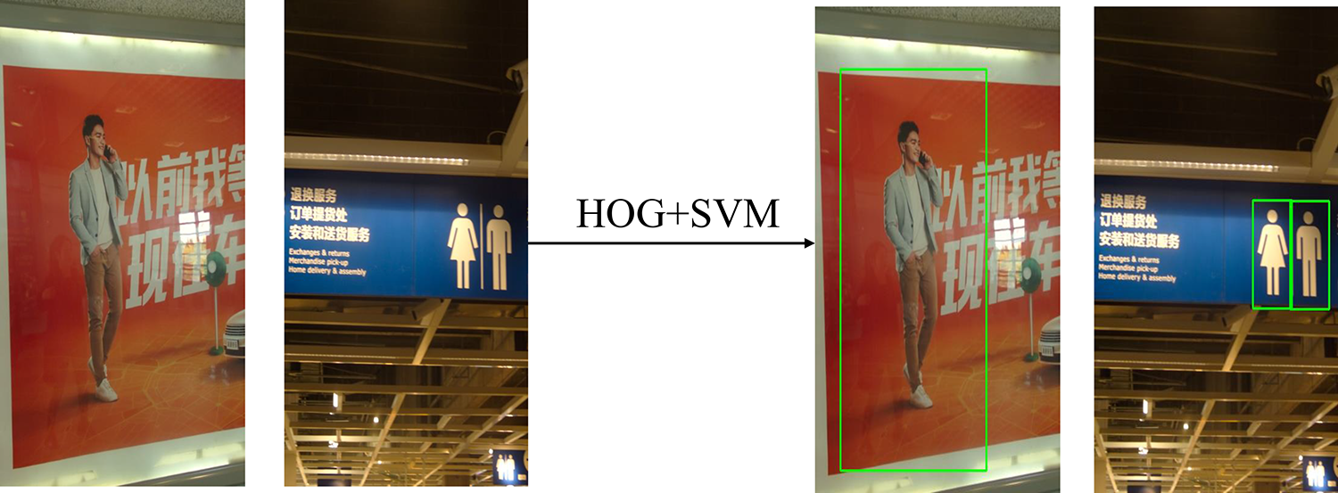
An example of detection results of HOG-SVM detector.

To solve the problem of the lack of stereo information in pedestrian recognition or detection tasks, many methods are proposed to utilize RGB-D or multispectral sensors for detecting pedestrian in various situations. Choi et al. used Kinect to detect people in the living room.⁸ Hsieh et al. presented a people counting system with Kinect achieving almost 100% bidirectional counting and real-time detecting.⁹ Chen et al. detected people in crowded scenes by fusing RGB and depth images from Kinect.¹⁰ Premebida and Nunes used the context-based multisensor for pedestrian detection in an urban environment.¹¹ Zhang and Tao proposed a pedestrian codetection framework for detecting pedestrians in binocular stereo sequence.¹² Park et al. proposed a novel sensor fusion convolutional neural network (CNN) framework for detecting pedestrians and improved the detection performance in the night.¹³ However, these methods are energy-consuming and inconvenient. For instance, the Kinect camera needs portable power and bracket when working outdoors, and the binocular vision systems need precise calibration to work well.

In the last decade, due to the fast development of microlens manufacturing, the light-field (LF) imaging techniques have been grown up in recent years, and commercial LF cameras have been put into the market such as Lytro¹⁴ and Raytrix.¹⁵ It gains more attention in the field of computer vision for its distinctive light recording and refocusing capabilities. Compared with traditional cameras, a LF camera is able to sample more (15 × 15 slices for Lytro Illum camera) 2D photos from different viewpoints. In contrast, traditional cameras only record one picture from one viewpoint at a given time. As a result, the depth estimation of the LF imaging has a certain development,¹⁶ and it makes many applications possible, for example, 3D scene reconstruction,¹⁷ image super-resolution reconstruction, and so on.¹⁸ Considering the unique imaging process of LF camera, it records both light intensity and the direction of each ray simultaneously. And thus, 2D RGB image and depth information can be captured with only one sensor in a single photographic exposure. So, using the LF camera is a better choice to solve the above problems in fact. We focus on a pedestrian recognition problem that we can use the depth information of the LF image to help the detector to recognize the pedestrians.

Given the above discussion, one question comes up naturally: how to utilize the 2D RGB and the depth information to assist pedestrian recognition. In this article, we aim to answer this question and explore the effects of different features on recognition results. This article contributes to:

We extend the LF pedestrian dataset¹⁹ to 1500 samples and add more scenes (such as shopping malls and shopping streets).

A unified CNN architecture is first proposed for the task of 2D fake pedestrian recognition based on LF imaging. And this network can be learned in an end-to-end manner.

The experimental results show that our proposed method exceeds the previous method¹⁹ on our dataset. It proves that our method is more suitable for this task and more advanced.

Related work

Light-field camera

Conventional digital cameras cannot record most of the information about the light distribution entering the world. So, it can only capture the 2D image and lack depth information. To solve the above problem, the first LF imaging is introduced by Adelson and Wang.²⁰ They construct a plenoptic camera using a lenticular array. The effect of the lenticular is to maintain the structure of light on the sensor array. Ng et al. invented the first handheld device and introduced digital refocusing, marking the birth of the LF camera.²¹ Moreover, Veeraraghavan et al. enriched the framework for obtaining the 4D information from LF camera and widened the application scope of the LF camera.²² Recent years, many new theories on LF camera application have been putting forward. Zhao et al. believed that a LF camera can be applied to the depth extraction of low-texture region.²³ Shi et al. introduced a novel technique that can simultaneously measure 3D model geometry and 3D surface pressure with a single LF camera.²⁴ Wang et al. proposed several novel CNN architectures to recognize the material on a 4D LF material dataset.²⁵ Fan and Yang estimated the depth of real-world scenes containing an object semisubmerged in water using a LF camera.²⁶

Pedestrian recognition

Traditional pedestrian detectors filter various integral channel features²⁷ before feeding them into a boosted decision forest, predominating the field of pedestrian detection for years. With the prevalence of deep CNN, CNN-based models^28,29 have pushed pedestrian detection results to an unprecedented level. Prior work by Park et al. embedded optical flow into a boosted decision forest to improve pedestrian detectors working on video clips.³⁰ Wang et al. proposed a novel loss function that improved the performance of the detector under occlusion cases.³¹ Liu et al. proposed an asymptotic localization fitting module based on the single stage detectors to improve the performance of pedestrian detection by continuously improving the accuracy of bounding box.³² Our previous work¹⁹ used the SVM classifier and the HOG⁷ descriptor to classify the pedestrian. The method in the article¹⁹ belongs to the traditional feature classifier architecture. To keep up with the current academic research and improve the accuracy of the whole system, we use the popular CNN³³ framework to identify the pedestrian from confused planar objects.

Proposed method

Light-field imaging and dataset

As shown in Figure 2(a), the LF camera consists of three parts: main lens, microlens array, and photosensor. Microlens array is a 2D array composed of multiple microlens units. The pupil plane (UV plane) of the main lens and the photosensitive plane of the image sensor are conjugating with respect to the microlens array (st plane). That is to say, the light passing through each microlens unit will be projected onto the image sensor to form a small microlens image. Each microlens image contains several pixels. At the same time, the light intensity recorded by each pixel comes from the narrow beam, which is limited by a space composed of a microlens and a main lens. As shown in Figure 2(b), the narrow beam here is the discrete sampling form of the LF. And the position and direction of each narrow beam can be determined by the coordinate (s, t) of microlens unit and the coordinate (u, v) of subaperture. Furthermore, the light distribution L(u, v, s, t) can be obtained.

Figure 2.

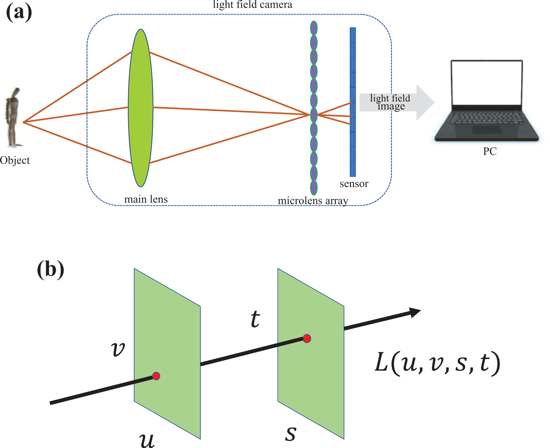
Light-field imaging: (a) schematic structure of a microlens-based LF camera and (b) two-plane parameterization model. LF: light-field.

Similar to the article,¹⁹ Lytro-Illum camera is adopted to capture the image. The Lytro camera is precalibrated at the factory, so we do not need to calibrate the camera when shooting the image. The spatial resolution of the Lytro camera is 376 × 541, and the angular resolution is 14 × 14. To train deeper CNNs, we expand the LF dataset to 1500 samples. It contains 750 positive samples and 750 negative samples. The raw data exported from the Lytro-Illum camera is saved in LFR format. Lytro official software is adopted for extracting the depth image and the RGB image.

Proposed scheme

We utilize the RGB and depth information extracted from the LF image to recognize the pedestrian image. Jeon et al. introduced an excellent method to evaluate the depth information from the raw LF image.¹⁶ However, the algorithm in the article¹⁶ is very time consuming, so we choose the official software (Lytro Desktop Application, ver 5.0.1),¹⁴ which is efficient for our dataset to extract depth image.

Our CNN architecture is shown in Figure 3. This system consists of three components: an RGB feature extraction network, a depth feature extraction network, and a classification network for the final recognition task. From the very left, the raw LF image is extracted as an RGB image and a depth image. The RGB image is feed into multiple convolutional layers, which are a part of the ResNet-50 pretrained model. The extracted RGB feature is denoted as X ₁. Correspondingly, the depth feature X ₂ is also extracted by feeding the depth image into some continuous convolutional layers. In classification network, RGB feature and depth feature are weighted and added linearly to get the final feature X for classification.

Figure 3.

Our proposed method consists of three components, including an RGB feature extraction network, a depth feature extraction network, and a classification network. k: the number of convolutional layers; X ₁: RGB feature; X ₂: depth feature;w ₁: the weight assign to X ₁; w ₂: the weight assign to X ₂.

RGB feature extraction network

As our dataset compared to the PASCAL VOC³⁴ and Cifar-10 is relatively small, it is not suitable to train from scratch. According to the relevance of recognition tasks, transfer learning strategy can be adopted for our recognition task. The model of VGG-16³⁵ and ResNet-50³⁶ trained on the ImageNet is commonly used model for recognition or detection tasks. In this article, we use the ResNet-50 pretrained model to extract the convolutional feature in the RGB feature extraction network. First, we release the last two layers of the ResNet-50 (average pooling and fully connected layer). Then, we fine-tune the parameters in the last convolution block of ResNet-50. This strategy not only makes use of existing knowledge trained on large-scale datasets but also adapts to specific datasets by updating the parameters of the convolutional layer. The extracted RGB convolutional feature is noted as X ₁.

Depth feature extraction network

Because the depth image is grayscale and its features are more evident than that of an RGB image, the prior knowledge based on the pretrained model cannot be used. To integrate with the overall network, we only need to construct several simple convolutional layers to extract features and the number of convolutional layers is noted as k. The extracted depth convolutional feature is noted as X ₂.

Classification network

As X ₁ and X ₂ play different roles in the recognition task, we assign different weights to each feature and then add them up to a mixed feature. It can be expressed as

X = w_{1} X_{1} + w_{2} X_{2}

where $w_{1} \in [0, 1]$ and $w_{2} \in [0, 1]$ . And w ₁ and w ₂ can be generated by the uniform distribution. The value of w ₁ and w ₂ can be updated with the backpropagation of neural networks. Finally, we feed the mixed feature X into the fully connected layers and the classification result can be obtained.

Experimental results and discussion

Experimental settings

Our framework was implemented using the Keras deep learning library. We trained the network using an Nvidia GeForce GTX 1080Ti GPU and adjusted the learning rate from 0.01 to 0.001 after 60 k iterations (in total 120 k iterations). We chose the 960 samples as our training set, which contained 480 positive images and 480 negative images, 160 samples as our validation set with 80 positive images and 80 negative images, and 380 samples as our test set with positive 190 samples and the 190 positive samples.

Experimental settings

To determine the value of k in the depth feature extraction network, we conducted a series of experiments to evaluate the effect of k on final results. We fed depth images into k convolutional layers. The value of k was set from 1 to 5. The experiment shows that if k equals to 3 or 4, we can get useful information from the feature map. As shown in Figure 4(b), the feature map enhanced stronger information and weakened some background information. And if the value of k exceeds 4, the feature map cannot present useful information.

Figure 4.

Depth image and feature map of some samples: (a) original depth image, (b) feature map if k = 3, and (c) feature map if k > 4.

As presented in Table 1, if k equals 3, the best recognition accuracy can be obtained. If k equals 5 or 6, the accuracy will decrease a lot. Therefore, in this experiment, only three convolutional layers are needed to obtain the optimal depth feature. The parameters of each convolutional layer in the depth feature extraction network are presented in Table 2.

Table 1.

The effect of different k on accuracy.

k	1	2	3	4	5	6
Accuracy	90.3%	93.1%	97.0%	95.5%	87.5%	87.2%

Table 2.

The parameters of each convolutional layer in the depth feature extraction network.

	Kernel_size	Stride	Padding	Out_channels
Conv1	3	1	1	6
Conv2	3	1	1	16
Conv3	3	1	1	32

As to the classification network, it contains an average pooling layer and a fully connected layer. The parameters are presented in Table 3.

Table 3.

The parameters of each convolutional layer in the depth feature extraction network.

AvgPool2d	Kernel_size	Stride	Padding
AvgPool2d	7	1	0
Fully connected	In_features	Out_features	Bias
Fully connected	2048	2	True

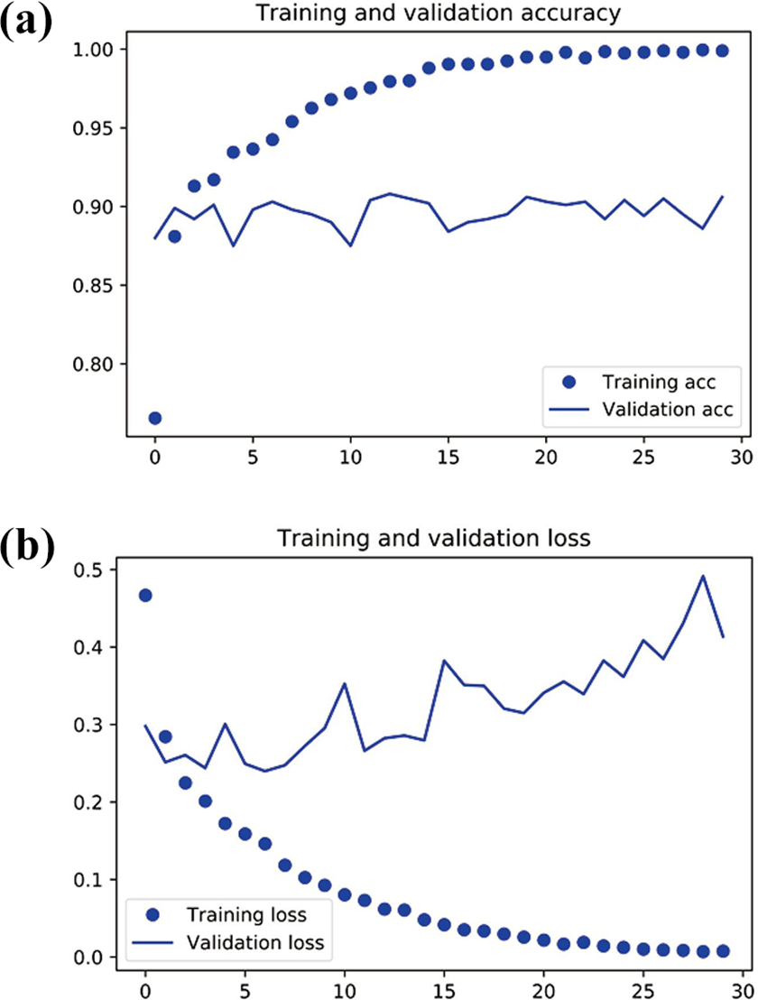
To illustrate the robustness and credibility of our training process, the curves of loss and accuracy during training are shown in Figure 5. The training accuracy increases linearly over time, until it reaches nearly 100%, while our validation accuracy stalls at 70–72%. Our validation loss reaches its minimum after only five epochs then stalls, while the training loss keeps decreasing linearly until it reaches nearly 0.

Figure 5.

(a)The curve graph of training and validation accuracy with training epochs variation. (b) The curve graph of training and validation loss with training epochs variation. X coordinate represents the epochs and Y coordinate represents the accuracy.

Because there are few samples in training set, overfitting is going to be our number one concern. According to Krizhevsky et al.,³⁷ data argumentation is a very useful trick to enhance performance. In this experiment, several data argumentation strategies are used, including rotation, channel shift, width, and height shift to reduce overfitting.

The Nesterov optimizer is also chosen instead of the common SGD optimizer in the whole proposed network according to the article.³⁸ As shown in Figure 6(a), the validation accuracy is about 90%. This result shows that the overfitting phenomenon is eliminated in the training process by adopting the above strategies. To illustrate the role of the depth feature extraction network, we conduct some comparison experiments, which only consist of an RGB feature extraction network. Similarly, to explain the effect of different pretrained classification accuracy, VGG-16 and VGG-19 pretrained model are adopted to evaluate it.

Figure 6.

As presented in Table 4, compared with the RGB network, the results of using the RGB + Depth network has improved significantly. It is proved that the depth information is helpful to improve the accuracy and is very necessary for the whole system. The pretrained models also have a relative impact on the experimental results. The ResNet-50 pretrained model is a highly efficient model in the ImageNet image classification tasks, and it is also suitable for our identification task. So, the ResNet-50 pretrained model is the first choice in the proposed architecture.

Table 4.

The test accuracy of using different pretrained models and networks.

Type Model	RGB + depth	Only RGB
VGG-16	96.1%	90.2%
VGG-16	96.1%	90.2%
ResNet-50	97.0%	91.1%

As given in Table 4, compared with the RGB network, the results of using the RGB + depth network has improved significantly. It is proved that the depth information is helpful to improve the accuracy and is very necessary for the whole system. The pretrained models also have a relative impact on the experimental results. The ResNet-50 pretrained model is a highly efficient model in the ImageNet image classification tasks, and it is also suitable for our identification task. So, the ResNet-50 pretrained model is the first choice in the proposed architecture.

To evaluate the effect of the depth-only model on the result, we conduct experiments only using the depth network. The recognition accuracy is only 70.2%. In some cases, the depth image is greatly affected by the surrounding environment. For example, in Figure 7, some of the pedestrian’s outlines are mixed with the ground, and some are not obvious to the background.

Figure 7.

(a, b) Some examples of depth images.

To illustrate the role of depth features in our experiments more intuitively, we list the classification probability of several cases in the test set in Figure 8.

Figure 8.

Some examples of the recognition results. (a) Real pedestrian, (b) LCD image, (c) advertisement board, (d) photo, (e) traffic signs, and (f) human model.

As shown in Figure 8(a), the real pedestrian gets a correct recognition result. Figure 8(b) shows that the pedestrian in the 2D screen and the recognition result is correct. The display board, photo, and traffic sign in Figure 8(c) to (e) are also recognized as the false pedestrian, so the result is correct. Figure 8(b) to (e) shows that depth images help the classifier to avoid being misled by the image in a 2D plane. Overall, depth images are very important to the final result in our dataset. The human model is recognized as the real pedestrian in Figure 8(f), so the result is wrong. It is a defect that our system cannot recognize the human models correctly. Because human models and human beings have the same shape and depth information, they have the same convolutional features. So, no matter what kind of pretrained models are chosen, the human models will always deceive the classifier in our proposed method.

Overall, our proposed method can solve most of the 2D fake pedestrian recognition problems. It makes full use of the features of the LF image to recognize the pedestrian. But in some cases, some LF images (human models) will deceive the classifier.

Conclusion

In summary, we expand the LF pedestrian dataset to 1500 samples and add more scenes like shopping malls and shop streets for increasing the applicability of our method. Since LF camera can obtain the information of whole 4D space, it can obtain the RGB information and depth information of an object at the same time in one exposure. In view of this, we exploit the recent success in deep learning approaches and train a CNN on this dataset to perform 2D fake pedestrian recognition. For RGB image, we adopt the resnet-50 pretrained models to extract the RGB features. For depth image, we design several convolutional layers for extracting depth features. These architectures provide insights to LF researchers interested in adopting CNNs and may also be generalized to other tasks involving LFs in the future. Our experimental results show that we can benefit from using 4D LF images and achieve a 5.9% boost compared with 2D image classification. We also analyze the role of RGB and depth information in the recognition results. Moreover, the proposed method can be easily integrated into pedestrian detection system. Finally, although we use this dataset for pedestrian recognition, it can also promote research on other applications that combine learning techniques with LF images.

Footnotes

Declaration of conflicting interests

The author(s) declared no potential conflicts of interest with respect to the research, authorship, and/or publication of this article.

Funding

The author(s) disclosed receipt of the following financial support for the research, authorship, and/or publication of this article: This work was supported by the National Key R&D Program of China [2018YFB1305200] and National Natural Science Foundation of China [No.62020106004, No.92048301, No.61906133, No.61703304, and No.61906134].

References

Xia

X-M

Jiang

Z-L

P-F

. A detection algorithm of spatter on welding plate surface based on machine vision. Optoelectron Lett 2019; 15(1): 52–56.

Wang

Zhou

. Pedestrian and cyclist detection based on deep neural network fast R-CNN. Int J Adv Robot Syst 2019; 16(2): 1–10.

Pang

Cao

Wang

, et al. JCS-Net: joint classification and super-resolution network for small-scale pedestrian detection in surveillance images. IEEE Trans Inf Forensics Secur 2019; 14(12): 3322–3331.

Zhao

Yuan

Chen

. Accurate pedestrian detection by human pose regression. IEEE Trans Image Process 2020; 29: 1591–1605.

Guo

Zhao

, et al. Pedestrian tracking based on Camshift with Kalman prediction for autonomous vehicles. Int J Adv Robot Syst 2016; 13(3): 120.

Cai

Wang

, et al. Pedestrian detection algorithm in traffic scene based on weakly supervised hierarchical deep model. Int J Adv Robot Syst 2017; 14(1): 1729881417692311.

Dalal

Triggs

. Histograms of oriented gradients for human detection. In: Proceedings of the IEEE conference on computer vision and pattern recognition (CVPR), San Diego, CA, USA, 20–25 June 2005, pp. 886–893. IEEE.

Choi

Pantofaru

Savarese

. Detecting and tracking people using an RGB-D camera via multiple detector fusion. In: IEEE international conference on computer vision workshops (ICCV Workshops), Barcelona, Spain, 6–13 November 2011, pp. 1076–1083. IEEE.

Hsieh

Wang

, et al. A Kinect-based people-flow counting system. In: International symposium on intelligent signal processing and communications systems, Taipei, Taiwan, 4–7 November 2012, pp. 146–150. IEEE.

10.

Chen

Henrickson

Wang

. Kinect-based pedestrian detection for crowded scenes. Comput-Aided Civ Inf 2016; 31: 229–240.

11.

Premebida

Nunes

. Fusing lidar, camera and semantic information: a context-based approach for pedestrian detection. Int J Robot Res 2013; 32(3): 371–384.

12.

Zhang

Tao

. Pedestrian detection in binocular stereo sequence based on appearance consistency. IEEE Trans Circuits Syst Video Technol 2016; 26(9): 1772–1785.

13.

Park

Kim

Sohn

. Unified multi-spectral pedestrian detection based on probabilistic fusion networks. Pattern Recognit 2018; 80(4): 143–155.

14.

. Lytro redefines photography with light field cameras, http://www.lytro.com/ (2014, accessed 18 October 2018).

15.

Perwass

Wietzke

. The next generation of photography. http://www.raytrix.de (2010, accessed 20 October 2020).

16.

Jeon

Park

Choe

, et al. Accurate depth map estimation from a lenslet light field camera. In: Proceedings of the IEEE conference on computer vision and pattern recognition (CVPR), Boston, MA, USA, 7–12 June 2015, pp. 1547–1555. IEEE.

17.

Kim

Zimmer

Pritch

, et al. Scene reconstruction from high spatio-angular resolution light fields. ACM Trans Graph 2013; 32(4): 1–12.

18.

Yoon

Jeon

Yoo

, et al. Learning a deep convolutional network for light-field image super-resolution. In: IEEE international conference on computer vision workshop (ICCVW), Santiago, Chile, 7–13 December 2015, pp. 57–65. IEEE.

19.

Jia

Shi

Zhao

, et al. Identification of pedestrians from confused planar objects using light field imaging. IEEE Access 2018; 6: 39375–39384.

20.

Adelson

Wang

JYA

. Single lens stereo with a plenoptic camera. IEEE Trans Pattern Anal Mach Intell 1992; 14(2): 99–106.

21.

Levoy

Bredif

, et al. Light field photography with a hand-held plenoptic camera. PhD Thesis, Stanford, CA: Tech. Rep. CSTR, 2005.

22.

Veeraraghavan

Raskar

Agrawal

, et al. Dappled photography: mask enhanced cameras for heterodyned light fields and coded aperture refocusing. ACM Trans Graph 2007; 26(3): 69–76.

23.

Zhao

Miao

Peng

, et al. Depth extraction of low-texture region using a light field camera. Opt Eng 2017; 56(7): 65–75.

24.

Shi

Zhao

, et al. 3D surface pressure measurement with single light-field camera and pressure-sensitive paint. Exp Fluids 2018; 59(5): 79.

25.

Wang

Zhu

Hiroaki

, et al. A 4D light-field dataset and CNN architectures for material recognition. In: European conference on computer vision, Amsterdam, the Netherlands, 8 October 2016, pp. 121–138. Springer International Publishing.

26.

Fan

Yang

. Depth estimation of semi-submerged objects using a light-field camera. In: 2017 14th conference on computer and robot vision (CRV), Edmonton, Alberta, Canada, 16–19 May 2017, pp. 80–86. IEEE.

27.

Doll´ar

Perona

, et al. Integral channel features. In: British machine vision conference (BMVC), London, UK, 7–10 September 2009. BMVA.

28.

Liang

Shen

, et al. Scale-aware fast R-CNN for pedestrian detection. IEEE Trans Multimedia 2018; 20(4): 985–996.

29.

Cai

Fan

Feris

, et al. A unified multi-scale deep convolutional neural network for fast object detection. In: European conference on computer vision, Zurich, Switzerland, 6–12 September 2014, pp. 354–370. Springer International Publishing.

30.

Park

Zitnick

Ramanan

, et al. Exploring weak stabilization for motion feature extraction. In: Proceedings of the IEEE conference on computer vision and pattern recognition, Portland, OR, USA, 23–28 June 2013, pp. 2882–2889. IEEE.

31.

Wang

Xiao

Jiang

, et al. Repulsion loss: detecting pedestrians in a crowd. In: Proceedings of the IEEE conference on computer vision and pattern recognition (CVPR), Salt Lake City, UT, USA, 18–23 June 2018, pp. 7774–7783. IEEE.

32.

Liu

Liao

, et al. Learning efficient single-stage pedestrian detectors by asymptotic localization fitting. In: European conference on computer vision, Munich, Germany, 8–14 September 2018, pp. 643–659. Springer International Publishing.

33.

C-b

Gao

S-s

. Multi-focus image fusion with the all convolutional neural network. Optoelectron Lett 2018; 14(1): 71–75.

34.

Everingham

Van Gool

Williams

CKI

, et al. The pascal visual object classes (VOC) challenge. Int J Comput Vis 2010; 88(2): 303–338.

35.

Simonyan

Zisserman

. Very deep convolutional networks for large-scale image recognition. In: International conference on learning representations (ICLR), San Diega, CA, July 2015, pp. 1–14. IEEE.

36.

Zhang

Ren

, et al. Deep residual learning for image recognition. In: Proceedings of the IEEE conference on computer vision and pattern recognition (CVPR), Las Vegas, NV, USA, 27–30 June 2016, pp. 770–778. IEEE.

37.

Krizhevsky

Sutskever

Hinton

. Imagenet classification with deep convolutional neural networks. In: Proceedings of the 25th International Conference on Neural Information Processing Systems (NIPS), Lake Tahoe, NV, USA, 3–8 December 2012, pp. 1097–1105. Curran Associates Inc.

38.

Rosebrock

. Optimization methods and regularization, Chapter 9. Baltimore, MD, US: PyImageSearch, 2017. pp. 113.

Light-field imaging for distinguishing fake pedestrians using convolutional neural networks

Abstract

Keywords

Introduction

Related work

Light-field camera

Pedestrian recognition

Proposed method

Light-field imaging and dataset

Proposed scheme

RGB feature extraction network

Depth feature extraction network

Classification network

Experimental results and discussion

Experimental settings

Experimental settings

Conclusion

Footnotes

Declaration of conflicting interests

Funding

References