An improved bioinspired cognitive map-building system based on episodic memory recognition

Abstract

Before the cognitive map is generated through the fire of the rodent hippocampal spatial cells, mammals can obtain the outside knowledge through the visual information, which comes from the eyeball to the brain. The information is encoded and transferred to the two regions of the brain based on the fact of biophysiological research, which are known as “what” loop and “where” loop. In this article, we simulate an episodic memory recognition unit consisting of the integration of two-loop information, which is applied to building the accurate bioinspired spatial cognitive map of real environments. We employ the visual bag of word algorithm based on oriented Feature from Accelerated Segment Test and rotated Binary Robust Independent Elementary Features feature to build the “what” loop and the hippocampal spatial cells cognitive model, which comes from the front-end visual information input system to build the “where” loop. At the same time, the environmental cognitive map is a topological map containing information about place cell competition firing rate, oriented Feature from Accelerated Segment Test and rotated Binary Robust Independent Elementary Features feature descriptor, similarity of image retrieval, and relative location of cognitive map nodes. The simulation experiments and physical experiments in a mobile robot platform have been done to verify the environmental adaptability and robustness of the algorithm. This proposing algorithm would provide a foundation for further research on bioinspired navigation of robots.

Introduction

At present, mobile robot system has many achievements in environment simultaneous localization, mapping, and navigation based on the Bayesian probability algorithm, such as Kalman filter, particle filter, bundle adjustment, and graph optimization algorithm. ^{1 –3} However, current technology is still far from producing a robot that can perform daily tasks in a complex environment. These daily tasks require cognitive map and episodic memory. The brain mechanism to acquire and construct the internal spatial representation is known as cognitive map. Tolman’s three-maze navigation ⁴ experiment reveals that the navigation behavior of animals depends on the internal environment called cognitive map. ⁵ Meanwhile, episodic memory enables human to achieve cognitive task through self-experiences and plan the actions accordingly.

It is well known that the neuron groups giving rise to cognitive map and episodic memory reside in entorhinal–hippocampal region. In 1971, O’Keefe and Dostrovsky found that when an animal is in a specific space position, the fire frequency of the specific vertebra neuron is changed. This neuron is called place cell. ⁶ After that researchers have discovered a series of spatial expression cells called head direction cell, grid cell, boundary vector cell, and band cell. ^{7 –10} The finding of place cells in hippocampus, grid cells and boundary vector cells in entorhinal cortex, head direction cells, and band cells in multiple brain regions, the proposition of various cognitive strategies in the hippocampus, and the construction of a hippocampal structural neural network not only make scientists more and more aware of the spatial cognitive mechanism and navigation mechanism of mammals (including humans) ^11,12 but also have deep research of “brain GPS.” Although the brain “GPS” field still has many unknown knowledge, it is almost certain that the bioinspired cognitive navigation system of mammals not only is based on internal path integration but also involves external cognitive information and episodic memory of physical world. ¹³

Mammals are rich in visual, auditory, taste, olfactory, tactile, and other external senses. They get a large amount of data from the receiver at all times. The mammals’ brain, in particular, abstracts the perception of the whole environment from perceived information to form a cognition and memory and makes more complex activities based on this memory. According to the study of biological cognitive environment, mammals (rodent and human) can obtain the outside knowledge through the visual information, which comes from the eyeball to the brain. Ungerleider and Mishkin were the first to propose a model of cortical visual processing that made a distinction between vision for perception and vision for action; cortical visual areas in the primate brain are organized into two major pathways, each arising from the primary visual cortex, V1. ¹⁴ The first, known as the “where-pathway,” spreads from V1 dorsally to the parietal lobe. Its main function is coding the spatial location and motion information, processing different aspects of the spatial layout of the outside world, such as location, distance, relative position, position in egocentric space, and motion. The second ventral route was referred to as the “what-pathway,” its main function is processing episodic memory recognition task, allowing us to perceive and recognize shape, orientation, size, objects, faces, and text. In 1992/1995, David Milner and Mel Goodale proposed a two visual system model, proposing that the division of labor between the two streams might be better characterized as one between two modes of output rather than two modes of input (i.e. object vs. spatial vision). ¹⁵ They argued process and transmit visual information in quite different ways for the two streams. The ventral stream transforms visual inputs into perceptual representations that embody the enduring characteristics of objects and their spatial relations. These representations enable us to parse the scene and to think about objects and events in the visual world. In contrast, the dorsal stream’s job is to mediate the visual control of skilled actions, such as reaching and grasping, directed at objects in the world. To do this, the dorsal stream needs to register visual information about the goal object on a moment-to-moment basis, transforming this information into the appropriate coordinates for the effector being used. ¹⁶ Finally, the information of two passages is converged in the hippocampus and the entorhinal cortex. Then mammals can update the pose by fusing the external visual cognitive information and the self-location inspired by place cell, grid cell, and so on.

The representative bioinspired simultaneous localization and mapping (SLAM) algorithms are RatSLAM and Hierarchical Look-Ahead Trajectory Model (HiLAM). RatSLAM ¹⁷ can generalize a cognitive map by visual information and self-motion information made by pose cell, local view cell and experience map. HiLAM ¹⁸ can create a place cell map by goal-direction method to express the environment completely. These methods make a good achievement in the outdoor navigation environment. But the core-sensing information is derived from the visual odometer, which is greatly influenced by the outside world. It has a rapid accumulation of errors in a large environment. And the closed-loop detection method uses the image pixel-based scanning line intensity algorithm, which has poor robustness and poor environmental adaptability. What’s more these algorithms are not well adapted to the indoor environment, which requires more accurate measurement.

With the development of computer vision technology, more and more image processing techniques, which can accomplish feature detecting, descripting, and deduce information about the environment have been applied to the visual SLAM system. ^{19 –21} Feature from Accelerated Segment Test (FAST) ²² compares the intensity of a point of interest with the intensities on a circle around the point. A decision tree is learned to efficiently classify corner-like features. The advanced improved FAST detecting key point algorithm, ²³ named oriented FAST and rotated Binary Robust Independent Elementary Features (BRIEF) (ORB), provides an independent rotation. It can detect the key points at different scales. Choosing a fixed set of intensity test pairs with minimal correlation to offset the resulting variance loss. It has a good performance for the invariance of rotation, scales, illumination, and the low-cost computation.

Related work

Inspired by the achievements of the two passages converged in the hippocampus and the entorhinal cortex, neuron fire activities cell (place cell, grid cell, and so on), ORB algorithm, and bioinspired SLAM algorithm (RatSLAM and HiLAM), our system use the integration of motion information and visual-based motion information to build the “where” loop and use the visual bag of word algorithm-based ORB feature to build the “what” loop. In this article, we simulate an episodic memory recognition unit consisting of the integration of two-loop information, which is applied to building the accurate bioinspired spatial cognitive map of real environments. Our work is to model hippocampus and to integrate cognitive map, and episodic memory, so as to make the performance of the robotic system more human-like. Then we make an experiment to show our algorithm has a good improvement in visual odometer accuracy, closed-loop detection, and robust environment adaptability.

This article is structured as follows. The first section has introduced the background of bioinspired cognitive method and the visual processing method, then it discusses the purpose of this article. Our experiment platform and system are introduced in the second section. The front-end visual information input method will be shown in the third section. The cognitive mode of bioinspired model and closed-loop detection method will be discussed in the fourth section. The experimental results will then be shown in the fifth section and the sixth section give a conclusion.

System overview

Our mobile robot platform has a full navigation system, which made up of a mobile robot base, a red green blue-depth (RGB-D) camera, and a laptop. Turtlebot2 consists of the structure of the robot, which has a Kubuki robot move base. The robot move base is a low-cost, personal robot kit with open-source software, two motor encoders offer the odometer information, and one micro inertial measurement unit (MIMU) offers the angle information. We use RGB-D camera of the ASUSTeK computer (ASUS) to collect visual information in the environment. It was fixed to the top of the platform panel and used universal srial BUS (USB) connection for power supply and laptop connecting. We choose Alienware13 laptop which has an i7 6500U 2.5 GHz CPU and an NVIDIA GeForce GTX960 M graphics card and use rbot orating sstem (ROS) system to control robot move base, collect visual information, process the visual RGB, depth image, coordinate the visual and odometer information, and generate the cognitive map. You can see the mobile robot platform hardware in Figure 1.

Figure 1.

Mobile robot platform.

The overall framework of the whole bioinspired cognitive map-building system is shown in Figure 2. The system consists of main three parts: in “where” loop, camera collects RGB and depth image information; for image information, our system uses ORB algorithm to extract feature points in images; after the pose estimation, the obtained angle and linear velocity information is integrated with angle and linear velocity information collected by the raw odometry; “where” loop have two outputs, one is the ORB feature detected by the ORB feature input into the “what” loop and the other is to use visual processing, pose estimation, and raw odometry to output the angle and line velocity input into the continuous attractor network (CAN) model; CAN model receives the angle and linear velocity, injects into head direction cells and band cells of their own, and outputs the exact and robust location of the environment by place cells which are competed from grid cells, and location of the environment inputs “what” loop; “what” loop, which uses visual bag of word algorithm to ensure a more accurate loop detection, contributes the episodic memory recognition unit. Eventually, we use episodic memory recognition unit model to build a cognitive map.

Figure 2.

Overall framework.

Front-end visual input system

In visual SLAM system, visual processing is a very important part. The front-end visual information input based on feature detection algorithm is irreplaceable. The robot collects the image information of the environment through the RGB-D camera. In RatSLAM ¹⁷ and HiLAM ¹⁸ algorithm, a visual odometry algorithm is proposed called scanline intensity profile, which used to calculate the odometer information and generate the outside topological map. Scanline intensity profile is a one-dimensional (1-D) vector, which is the sum and normalization of the intensity of all the columns of the gray scale of the image pixels. However, it has a low robust performance at different light intensity at different periods of time and in the indoor environment. In our method, we exquisitely use ORB algorithm to extract feature points in images. These feature points will enter the following two aspects: pose estimating and loop closure detecting. They are the basis for the accurate results behind them.

In the ORB algorithm, the ORB operator performs the feature detection through the FAST algorithm while adding the direction information of the FAST feature. The BRIEF algorithm is used to describe the feature points, so that the ORB operator has rotation invariance, and it is not very sensitive to the image noise. What’s more, the multiscale invariance is also needed in the image processing. The multiscale space theory is used to extract stable feature points; at the same time, parameters are set for the number and spacing of feature points when feature detection is performed, so that ORB operators are scale-invariant and distributed uniformly, then the feature point description and matching will be completed next. ORB uses oFAST, which has good performance. The matrix of the image region is shown in the following equation

$m_{pq}={\displaystyle \sum }_{x, y}{x}^p{y}^{q}I\left(x, y\right)$

1

$x^p\hspace{0.17em}\text{and}\hspace{0.17em}{y}^q$ represent the coordinates of p and q, and is image grayscale expression. The centroid of this region is shown in the following equation

$C=\left(\frac{m_{10}}{m_{00}},\frac{m_{01}}{m_{00}}\right)$

2

The orientation of the FAST feature point is shown in the following equation

$\theta =\text{arctan}(m_{01},m_{10})$

3

After the direction information of the o-fast focus detection algorithm was improved, ORB algorithm also proposed the improved rBRIEF algorithm to address the shortcoming of the original BRIEF algorithm in the description of rotation invariance. Set a set of test points (x, y) with n test point pairs, so matrix S is shown in the following equation

$S=\left(\begin{array}{c}{x}_1,\dots ,x_n\\ y_1,\dots ,y_n\end{array}\right)$

4

A directional characteristic matrix is added to the set of measured points, get direction information from equation (5), so new descriptor is shown in equation (6)

$S_{\theta }=R_{\theta }S$

5

$g_n\left(p,\theta \right):=f_n\left(p\right)|\left(x_i,y_i\right)ϵS_{\theta }$

6

$R_{\theta }$ is rotation matrix of θ, and we construct a look-up table for key points orientation and views by discretizing the angle to increments of 12°. By look-up table, we can find the correct set of points $S_{\theta }$ .

Since the ORB operator is essentially a binary string, the Hamming distance is used to measure the matching degree. The smaller the value is, the higher the similarity is. And the Hamming distance is the number of the different characters in the corresponding position of the two ORB operators. But in general, there will be mismatched point pairs, which make the matching of the feature points inaccurate. So the random sampling uniform algorithm Random Sample Consensus (RANSAC) is used to eliminate mismatched point pairs.

Specific steps for ORB feature scene-aware matching are shown in Figure 3(a): The first two images are used as experimental samples for two laboratory indoor raw data images and the last image is the output image after feature extraction for one of the images. The circle in the image is the feature point, and the radius of the circle represents the radius of the descriptor; Figure 3(b): Using the original ORB feature for feature matching images, it can be seen that the whole matching result is messy and there are many mismatches; and Figure 3(c): The RANSAC algorithm is used to remove the mismatched situations, and the sampling consistency is used to improve the stability of the matching.

Figure 3.

(a)–(c) ORB feature scene-aware matching. ORB: oriented Feature from Accelerated Segment Test and rotated Binary Robust Independent Elementary Features.

Then a stable six-pair point set is selected to use the Efficient Perspective-n-Point algorithm, ²⁴ and as in equation (8), solve the interframe pose motion which is represented by rotation matrix R ^3×3 and translation matrix t ^3×1. In the end, the angular velocity and linear velocity of the robot can be obtained by using Rodrigues’ formula. Then we integrate raw odometry with this part of the information, as in equation (11), and complete the front-end visual input loop. Comparing with the other feature operator such as scale-invariant feature transform and speeded up robust features, the ORB operator has an advantage in calculation speed, rotation, scale invariance, and robust pose estimation

$s\left(\begin{array}{c}{u}_1\\ v_1\\ 1\end{array}\right)=\left(\begin{array}{c}{t}_1\\ t_5\\ t_9\end{array}\begin{array}{c}{t}_2\\ t_6\\ t_{10}\end{array}\begin{array}{c}{t}_3\\ t_7\\ t_{11}\end{array}\begin{array}{c}{t}_4\\ t_8\end{array}\right)\left(\begin{array}{c}\begin{array}{c}X\\ Y\end{array}\\ Z\\ 1\end{array}\right)=\left(\begin{array}{cc}{R}^{3\times 3}& t^{3\times 1}\end{array}\right)\left(\begin{array}{c}\begin{array}{c}X\\ Y\end{array}\\ Z\\ 1\end{array}\right)$

7

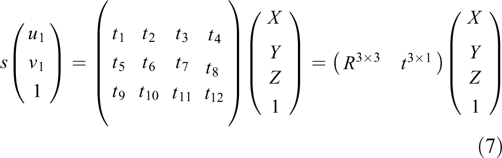
where (X, Y, Z, 1) is the homogeneous coordinate of point P and (u ₁, v ₁, 1) is projection feature point obtained by camera projection. Matrix $\begin{array}{cc}{R}^{3\times 3}& t^{3\times 1}\end{array}$ can be obtained by direct linear transformation and shown in the following equation

$\left(\begin{array}{c}\begin{array}{ccc}{P}_1^T& 0& -u_1{P}_1^T\\ 0& P_1^T& -v_1{P}_1^T\end{array}\\ \begin{array}{ccc}⋮& ⋮& ⋮\end{array}\\ \begin{array}{ccc}{P}_N^T& 0& -u_N{P}_N^T\end{array}\\ \begin{array}{ccc}0& P_N^T& -v_N{P}_N^T\end{array}\end{array}\right)\left(\begin{array}{c}{t}_1\\ t_2\\ t_3\end{array}\right)=0$

8

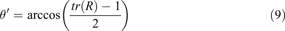
The velocity and angle models of the robot are constructed by the uniform motion state of the robot, and the velocity v′ and angle θ′ are obtained by Rodrigues’ formula

${\theta }^{\prime }=\text{arccos}\left(\frac{tr\left(R\right)-1}{2}\right)$

9

$v^{\prime }=\frac{\sqrt{{\left({t^{\prime }}_4-t_4\right)}^2+{\left({t^{\prime }}_8-t_8\right)}^2+{\left({t^{\prime }}_{12}-t_{12}\right)}^2}}{t}$

10

We use θ′ and v′ to correct the raw odometry information θ″ and v″, corrected velocity and angle are shown in the following equation

$\text{θ}={\theta }^{″}+\alpha {\theta }^{\prime },v=v^{″}+\alpha v^{\prime }\left(\alpha \in \left(0,1\right)\right)$

11

$\alpha \in \left(0,1\right)$ is the weighting coefficient, by equation (11), we can reduce errors in the raw odometry.

After the front-end visual input system, the robot obtains accurate angle and line velocity . Then the information is inputted into the next CAN cognitive model to form a cognitive map.

Cognitive mode

Cognitive mode is mainly composed of the following parts: CAN cognitive model, closed-loop detection, episodic memory recognition unit model, and cognitive map. We discuss these parts in detail in this section.

CAN cognitive model

The whole model contains four parts: head direction cell, band cell, grid cell, and place cell. The CAN cognitive model is different from these proposing methods. ^25,26

Head direction cell

Head direction cell is important for the movement of the animal. Head direction cells code the direction of the rat’s movement, and when all the information from head direction cells came together, t, a continuous head-direction signal, is generated. Head direction cell has a maximum fire rate when the animal’s head faces its preference angle. Based on the fact of biophysiological research, the regulation equations of head direction cell for the velocity signal are obtained as in the following equation

$D\left(t\right)=v(t)\left[\begin{array}{ccc}\text{cos}\left({\theta }_1+{\theta }_0\right)& \dots & \text{cos}\left({\theta }_m+{\theta }_0\right)\\ \text{sin}\left({\theta }_1+{\theta }_0\right)& \dots & \text{sin}\left({\theta }_m+{\theta }_0\right)\end{array}\right]$

12

The priority direction of head direction cell i can be expressed as a major orientation θ₀ and an angular offset θ_i that the range of value is 0°–360°

Band cell

Before forming grid cell layer, band cells are encoded as displacement in a specific direction. Band cells fire activity is a periodic reset encoding process and is responsible for path integration of line velocity.

$v_{\theta }\left(t\right)=\text{cos}(\theta -\omega (t))v(t)$

13

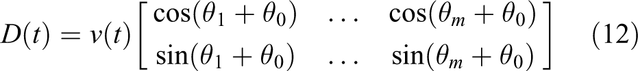
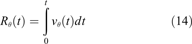
The θ is its preference direction. At t time, the velocity of the robot moving along the ω(t) direction is v(t). At this point, the shift of the velocity in direction is shown in the following equation

$R_{\theta }\left(t\right)=\underset{0}{\overset{t}{{\displaystyle \int }}}{v}_{\theta }\left(t\right)dt$

14

We can calculate the fire rate of band cell, which uses the Gauss fire model and shows it in the following equation

$F_{\theta }\left(t\right)=e^{\frac{-{\left(\left(\left(R_{\theta }\left(t\right)-\beta \right)\text{ mod }f\right)-\left(\frac{f}{2}\right)\right)}^2}{b}}$

15

where β is its phase and f is its firing cycle. As the forward input of grid cell attractor model, band cells are the coupling of the input signals, and the direction of grid cell attractor is determined.

Grid cell

In the process of animal exploration, grid cells fire periodically, forming hexagonal fire fields to cover the whole environment, and their fire activities are highly stable. The connection between the cells of the grid is inhibitory; the fire activity is regulated by the signal of head direction cells and band cells in the entorhinal cortex and hippocampus. Grid cells receive the forward projection from band cells, and the preferential orientation information in the forward projection is used to determine the direction of change of the output weight and determine the speed input information of the mouse it receives. So the recursive weights between grid cells are shown in the following equation

$w_{ij}^{\text{grid}}=\left(a{e}^{-\gamma {\left|x\right|}^2}-e^{-\beta {\left|x\right|}^2}\right)\left(x_i-x_j-S_{\theta }\left(t\right)\right)$

16

The distribution of a Mexico cap represents grid cell connection weights. In program initialization, $\gamma =1.05\times \beta$ and $\beta =3/{\lambda }_{\text{grid}}^2$ . Where ${\lambda }_{\text{grid}}^{}$ denotes the period of forming a grid on a neural lamella. Then the preliminarily integrated motion information is replaced by grid cell response equation to further integrate grid cell response. Interconnections between grid cells are inhibitory, each grid cell neuron receives inhibitory input from surrounding annular local neurons, and the entire network receives forward excitatory projections from the upstream cortex. The dynamic formula of grid cell response is shown in the following equation

$T\frac{d{S}_i}{dt}+s_i=f\left[{\displaystyle \sum }_j{w}_{ij}^{\text{grid}}{s}_j+F_{\theta }\left(t\right)\right]$

17

$eg:f\left(x\right)=\left\{\begin{array}{c}x, x>0\\ 0, x\le 0\end{array}\right.$

18

s_j  is the current state of the neuron i. $w_{ij}^{\text{grid}}{s}_j$ is the inhibitory input which is from neuron to neuron j. $F_{\theta }\left(t\right)$ is the forward input of band cell. f(x) is a rectified linear unit function. If the length of the neural plate is N, there are N ² neurons in the whole neural network. Each neuron has a prioritized direction. The priority information is determined by the projection of band cells.

Place cell

Place cells are capable of encoding the relative position of the space. It is the basic unit of the formation of cognitive map in the brain, and its fire activities provide a continuous and dynamic spatial position expression. A large number of place cells can be expressed in a discrete environment, thus establishing an end-to-end mapping relationship between the animal self-coordinate system and the physical world coordinate system.

Our team had built a competitive network from grid cells to place cells, which is used for self-organizing coding, which successfully simulates the characteristics of place cell field. Further through Hebb learning, a place cell field with a single peak is produced to simulate the place cell characteristics in CA3 (Cornu Ammonis3) region of hippocampus.

To generate a single-peak fire field of place cell cluster, it is necessary to learn the synaptic weight distribution of grid cells to place cells and determine the activation ratio of grid cell cluster with overlapping active packets at a single location. So using the Hebb learning rules, a competitive network model is built to find the set of grid cell activity

$\frac{d{w}_{ij}^{\text{place}}}{dt}=\alpha p_i\left(s_j-C_{\text{grid}}\right)$

19

α represents the learning rate. p_i is place cell fire rate. s_j is the inhibition of grid cell. If the excitement is greater than the inhibition, the weight connection will become stronger, and the opposite will be weak. At the same time, the cluster activity of place cells is derived from the projection information of grid cells; the fire function of multiple place cell cluster is shown in the following equation

$p_i=Af\left[{\displaystyle \sum }_{j=1}^M{w}_{ij}^{\text{place}}{s}_j(\text{r})-C_{\text{place}}\right]$

20

A and $C_{\text{place}}$ are the constants of the excitation and inhibition of place cell network, respectively. M is the layer number of neural plate. r represents the animal location of environment.

Place cell expression model

There is a mutual inhibition between place cells. The stronger the excitability of neuron cells, the stronger the inhibition of the surrounding neuron cells. Finally, a single fire field is formed in neuron cells. The movement of place cell attractor comes from the spatial cell’s integration of the path from the motion cues, including band cell encodes the displacement in a specific direction, drives the movement of grid cell attractor, and grid cell attractor encodes the two-dimensional (2-D) space in a specific direction, causing different grid cell clusters to activate, and a subset of different grid cell cluster activities determines the movement of place cell attractor.

Using 2-D Gauss distribution to create an excitatory weight connection matrix ${\epsilon }_{m,n}$ for place cell

${\epsilon }_{m,n}=e^{-(m^2+n^2)/k_p}$

21

where m and n denote the specific distance between the coordinate x and y. k_p is the constant of the position distribution.

The amount of place cell activity changes caused by local excitatory connections is shown in the following equation

$\Delta P_{Ex,Ey}={{{\displaystyle \sum }}^{\text{}}}_{i=0}^{n_x-1}{{{\displaystyle \sum }}^{\text{}}}_{j=0}^{n_y-1}{p}_{i,j}{\epsilon }_{m,n}$

22

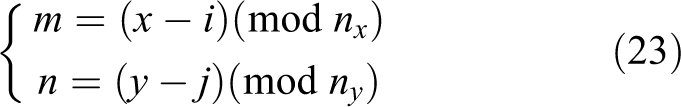
n_x and n_y are the number of (x, y) space in 2-D matrix of place cell. The premise of place cell iterative, closed-loop detection, and episodic memory recognition unit is to find the relative position of place cell attractor in the neuron plate. So the relative position is shown in the following equation

$\left\{\begin{array}{c}m=(x-i)(\text{mod} n_x)\\ n=(y-j)(\text{mod} n_y)\end{array}\right.$

23

In addition to the excitatory signal, the cells in each position accept the global inhibitory signal. The balance of excitability and inhibitory connection ensures proper neural network dynamics and the attractors in the space are not unrestrictedly excited. The activity of inhibitory connection weight is shown in the following equation

$\Delta P_{Ix,Iy}={{{\displaystyle \sum }}^{\text{}}}_{i=0}^{n_x}{{{\displaystyle \sum }}^{\text{}}}_{j=0}^{n_y}{p}_{i,\text{ j}}{\psi }_{m,n}-\phi$

24

${\psi }_{m,n}$ is the inhibition weight connection matrix. φ is the inhibitory constant. To make sure that the firing rates of all place cells are always positive, the activity rate of place cell is normalized and updated

$p_{x,y}^{t+1}=\frac{\text{max}\{p_{x,y}^t+\Delta P_{Ex,Ey}+\Delta P_{Ix,Iy},0\}}{{{{\displaystyle \sum }}^{\text{}}}_{i=0}^{n_x}{{\displaystyle \sum }}_{j=0}^{n_y}{p}_{ij}^t}$

25

Finally, place cells attractor movement is derived from the spatial cell to the path integration of the self-moving trajectory integral; the firing rate of place cells after grid cell path integration is shown in the following equation

$p_{x,y}^{t+1}=\underset{}{\overset{}{{\displaystyle {\displaystyle {\sum }_{m=\delta x_0}^{\delta x_0+1}{\displaystyle {\sum }_{n=\delta y_0}^{\delta y_0+1}{\alpha }_{mn}{p}_{(m+x)(n+y)}^t}}}}}$

26

The firing rate of place cell at the next time is determined by the firing rate of place cells at the current time and the residual. The residual α_mn is expressed by the following formula and shown in the following equation

${\alpha }_{mn}=H\left(\delta X_f,m-\delta X_0\right)H\left(\delta Y_f,n-\delta Y_0\right)$

27

$\text{eg}:H\left(x,y\right)=\left\{\begin{array}{c}1-x, y=0\\ x, y=1\end{array}\right.$

28

$\delta X_0$ and $\delta Y_0$ are offset of X–Y coordinate which determined by velocity and direction information and shown in equation (29). $\delta X_f$ and $\delta Y_f$ are the residual offset, which is the diffusion of the activity package of place cells and shown in equation (30)

$\left[\begin{array}{c}\delta X_0\\ \delta Y_0\end{array}\right]=\left[\begin{array}{c}{k}_m{\stackrel{\rightharpoonup }{e}}_{{\theta }_i}v\cdot \text{cos}\theta \\ k_n{\stackrel{\rightharpoonup }{e}}_{{\theta }_i}v\cdot \text{sin}\theta \end{array}\right]$

29

$\left[\begin{array}{c}\delta X_f\\ \delta Y_f\end{array}\right]=\left[\begin{array}{c}{k}_m{\stackrel{\rightharpoonup }{I}}_{{\theta }_i}v\cdot \text{cos}\theta -\delta X_0\\ k_n{\stackrel{\rightharpoonup }{I}}_{{\theta }_i}v\cdot \text{sin}\theta -\delta Y_0\end{array}\right]$

30

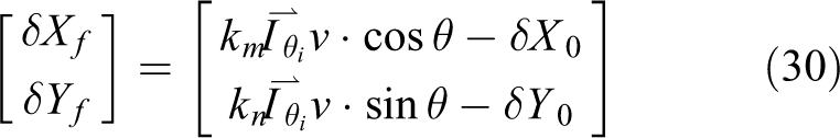
k_m and k_n is the path integral constant, ${\stackrel{\rightharpoonup }{e}}_{{\theta }_i}$ is a unit vector pointing to θ_i . It can be seen that a single position discharge field is eventually generated, which is more accurate and more consistent with biological research than the method proposing in the article. ²⁵ Because pose cells, the article ²⁵ uses are not real cells in biology, but imaginary cells, while grid cells and place cells we use, are physiologically discovered cells.

Closed-loop detection

Closed-loop detection is an important part of mapping. The inevitable accumulative error occurs during the operation of the robot. At the same time, when the robot runs for a period of time, the standard matching algorithm will fail when the long-time unobserved area is observed by the robot sensors. When these regions can be detected steadily, the closed-loop detection algorithm can provide the correct data association.

In computer vision field, visual word bag is a model with good applicability, which can be used for video or image retrieval. By extracting and describing the features of the image, the key words that represent the image are obtained, and a visual dictionary is built on this basis. Then the image can be similar to the text representation. We count the frequency of the basic words, represent the image into a vector, and use this vector to retrieve the image.

We use a binary ORB feature descriptor for feature extraction, clustering by k-majority algorithm, ²⁷ and finally get a tree of the eigenvector of an image.

The specific algorithm steps are shown as follows:

It is assumed that the set of ORB feature descriptors extracted from the image is D.

Step 1: Mark a set C generated randomly by K binary cluster centers. To construct binary visual word description vectors from image’s ORB feature descriptors, traditional clustering methods based on Euclidean distance such as k-means algorithm cannot directly cluster the vectors of visual words, so we use the Hamming distance in calculating the feature distance of the visual word vector.

Step 2: Calculate the distances from each descriptor to each cluster center C in the D and divide into a class.

Step 3: Recalculate each cluster centers.

Repeating step 2 and step 3 until the algorithm ends when the cluster centers are no longer changed.

The calculation method of cluster center is as follows:

Assuming that a set of D which contains N feature descriptors

$d_i=b_{i1}{b}_{i2},\dots ,b_{i256}$

31

Its cluster center is

$c=c_1{c}_2,\dots ,c_j,\dots ,c_{256}$

32

$\text{eg}:c_j=\left\{\begin{array}{c}0,{\displaystyle \sum }_{1\le i\le 256}{d}_{ij}<\frac{n}{2}\\ 1,{\displaystyle \sum }_{1\le i\le 256}{d}_{ij}>\frac{n}{2}\end{array}\right.$

33

For each image of the training set, each word in the word list is represented by $F_i(1\le i\le t)$ , calculating the frequency m_i of the appearance of F_i , t is the sum of visual word. Then calculating the image weight in word F_i which based on term frequency–inverse document frequency theory.

${\text{ω}}_i=m_i\times lg\frac{N}{n_i},(1\le i\le t)$

34

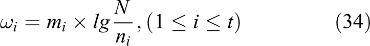
N is the number of all the words in the image, n_i is the number of selected words. At last, each image can be expressed as a word weight vector, which is shown in the following equation

$d_j={\omega }_{1,j},{\omega }_{2,j},\dots ,{\omega }_{t,j}$

35

Computing the definition of image differences. Degree of deviation S(d_i,q) is shown in the following equation

$\text{S}(d_i,\text{ q})={‖d_i-q‖}_p$

36

The two-norm is used here, so q = 2. Comparing the degree of difference between a query image and a trained image. Select the first n of the smallest difference as the result of the query image. After the closed-loop detection, the map will be more consistent with the external environment, generating a more robust, stable, and accurate map. This is an advantage over method. ²⁶

Episodic memory recognition unit and cognitive map

Cognitive map is a topological map, which contains many episodic memory recognition units. Episodic memory recognition unit is an episodic memory recognition network consisting of a number of discretely distributed units em_i . There is a connection weight ω between the units, and the transformation between the units is realized by the weight ω. In the cognitive map, the robot stores the scene perception of the current environment into episodic memory recognition unit. When the robot needs to perform object-oriented navigation based on episodic memory, according to the environment in which the robot is located, place cells firing degree after place cells renewal can be obtained by measuring the similarity between the scene perception in the current environment and all scene perceptions in the cognitive map, and comparing current place cells firing rate and all place cells firing rates information. Episodic memory recognition unit determines whether to establish a mapping relationship between the current location and a new scene or to associate the current location with the original scene. At the same time, the place cells will be periodically fired to reset to enable the robot to obtain the external scene and its own posture perception; the weights between episodic memory recognition units are learned and updated through a competitive neural network model. Different from traditional map units that only contain location information, episodic memory recognition unit contains spatial cells firing information and corresponding scene perception information, which can make the map update more flexible and contribute to the construction of a more accurate cognitive map.

The robot completes the position-sensing input of the robot through “where” loop and obtains the external environment position perception through the hippocampal CAN model, forming an environmentally stable expression unit em_i . At the same time, the robot maps the external scene perception to the environment expression unit em_i through the “what” loop to obtain specific environmental location information and episodic memory recognition information. As the robot traverses the entire environment, an external spatial representation formed by several units can be obtained, that is, episodic cognitive map. Each unit in cognitive map can be described as follows

$e{m}_i=\left\{p_i,S_i,L_i\right\}$

37

where em_i is the episodic memory recognition unit of cognitive map. The information of place cell p_i and the image information S_i which contains the ORB feature descriptors and the three pictures index of other maximum similarity are associated to em_i . L_i is the location of cognitive map.

When the fire rate of place cell is greater than 0.9, the image information S _i will be insert in the episodic memory recognition unit em_i . And a new unit is created

$e{m}_j=\left\{p_j,S_j,L_i+\Delta L_{ij}\right\}$

38

When closed-loop detection occurs in the process, the location of the episodic memory recognition unit in cognitive map $\Delta L_i$ is obtained by

$\Delta L_i=\text{α}\left[{\displaystyle \sum }_{j=1}^{N_f}\left(L_j-L_i-\Delta L_{ij}\right)+{\displaystyle \sum }_{k=1}^{N_t}\left(L_k-L_i-\Delta L_{ki}\right)\right]$

39

where α is correction rate constant, N_f is the number of transfers from the cognitive point em_i to the other cognitive points, and N_t is the opposite.

Experiment result

We explain the specific implementation and experiment of the algorithm in the following sections. First, we use an indoor picture set to test the closed-loop detection algorithm. Then we run the map-building algorithm in an indoor environment, giving the interaction between grid cells and place cells as well as the results of the cognitive map at last. Next, we compare the performance differences between our algorithm and the RatSLAM ¹⁷ algorithm. The contrastive data set comes from the open-source data set ²⁸ at the Queensland University of Technology in Australia.

Closed-loop detection

To verify the effectiveness of image retrieval proposed by this method, we made an indoor environmental data set containing two days and two nights of collection, using one daytime data set as the test set and the other three times as the training set, randomly selecting one of the three sets of images collected in the training set are shown in Figure 4(a) and marked the corresponding pictures that should be closed-loop detected. At the same time, we set up the corresponding threshold to control the point of closed-loop detection and reduce the false-positive loop-closure detection.

Figure 4.

(a)–(d) Example of image retrieval results.

First, we train visual words from the training set; the number of visual words is 46,449. Then, each picture is retrieved from the data in the test set. The results of the query are sorted according to the similarity. Because of the small size of experiment, the first three images are taken as the retrieval results. The retrieval results are shown in Figure 4. Three images for each line are retrieved. The first image in the retrieval result is the original image itself. The similarity between the original image and the retrieval result image is sorted from left to right. The left is high similarity and the right is low similarity.

Figure 4(b) presents the 33 s original image and the 210 s and 336 s retrieval result images, which happened the loop closure detection. Figure 4(c) presents the 18 s, 111 s, and 195 s images. Figure 4(d) presents the 150 s, 273 s, and 357 s images. The result shows that this closed-loop detection algorithm has a higher robustness and environmental adaptability than the image pixel-based scanning line intensity algorithm.

Congnitive map

We use a robot platform to build a map of the indoor lab, which contains a range of 17 m by 3 m, with a time of 372 s. The raw odometry obtained by front-end visual information input is shown as the left of Figure 5. Cognitive map is shown as the right of Figure 5. As we can see, the cognitive map in Figure 5(a) is fully similar to initial raw odometry. But as time goes on, the error of the raw odometry increases a lot, and the cognitive map is more and more conform to the real track after several closed-loop detections in Figure 5(b) to (d).

Figure 5.

The process of map building. (a) T = 71 s, (b) T = 173 s, (c) T = 275 s, and (d) T = 367 s.

At the same time, in this article, using the expression of head direction cells and band cells forwards drive grid cell attractor to express the location periodically. Place cell activity clusters are generated by the subset of grid cells, and the interaction between the place cells forms a single type of fire field which gets the expression of whole environment. This cognitive model produces a single peak fire field by the mutual competition of place cells; comparing with traditional SLAM method, the position in this article is expressed by spatial cell fire, which is more in line with the facts of biophysiological research. The right images of Figure 6 present multi-peak fire phenomenon, and the left of Figure 6 images show the single-peak fire field phenomenon.

Figure 6.

The fire rate of place cell after competition. (a) T = 3 s, (b) T = 71 s, and (c) T = 178 s.

Experimental comparison

The contrastive data set comes from the open-source data set ²⁸ at the Queensland University of Technology in Australia, which simulates an outdoor street environment. The iRat 2011 data set is taken indoors on a custom-embedded computer using a camera, mounted on a small custom robot, travelling at tenths of a meter per second, across an area covering only a few square meters. The data set includes a robot’s 953 s odometer and RGB image information that is explored in the environment. The experimental structure diagram is shown in Figure 7.

Figure 7.

Experimental structure.

The map constructed by our algorithm and RatSLAM running 15 min is shown in Figure 8. Comparing with the RatSLAM algorithm, our algorithm is more consistent with the original map and the map is more accurate under the same time. The time it takes for our algorithm and RatSLAM to generate a map that is almost identical to the original map such as Figure 8(right) is shown in Figure 9, our algorithm is better than RatSLAM in runtime. Because the collected data are a maze map, the nature of the maze ground means that the wheel odometer is prone to error, especially the accumulated errors caused by wheel skid. Our algorithm corrects the error very well, indicating that our algorithm has better environmental adaptability and robustness. Moreover, the navigation cells named pose cells used by RatSLAM to simulate rat navigation are artificial cells, not biological cells. Place cells and grid cells used in our algorithm are located in the hippocampus of the rat brain; they are real cells, so our algorithm is more suitable for the study of robot bionics.

Figure 8.

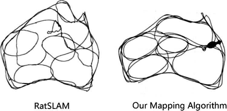
The comparison of result running 15 min between RatSLAM (left) and our mapping algorithm (right). SLAM: simultaneous localization and mapping.

Figure 9.

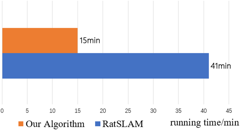
The comparison of running time between RatSLAM and our algorithm. SLAM: simultaneous localization and mapping.

Conclusion

In this article, we present a bioinspired cognitive map-building system based on episodic memory recognition. Inspired by the achievements of biophysiological research, we apply the motion information obtained from the front-end visual input system to neuron fire activities cells (place cells, grid cells, and so on). After obtaining the place unit of the spatial cell fire field, we integrate it with visual bag of word algorithm based on ORB feature and form an episodic memory recognition unit. The episodic memory recognition unit contains place cells fire information, position information in the corresponding environment, pose information of the robot at the next moment and the previous moment, topological information relative to the cognitive map, and episodic information in the environment. At last, an accurate cognitive map, which represents real physical space, is built. Compared to traditional SLAM, our algorithm uses spatial cells found in biology. Comparing with RatSLAM, our algorithm has a better performance in environmental adaptability and robustness; the whole algorithm framework is more consistent with the fact of biophysiological research. Instead of RatSLAM using fictitious cells, the cognitive map-building method proposing in this article is based entirely on the biophysiological mechanism, which lays the foundation for further research on bioinspired navigation of robots.