Sage Journals: Discover world-class research

Abstract

The proposed study presents an original concept for the design of a walking robot with a minimum number of motors. The robot has a simple design and control system, successfully moves by walking, avoids or overcomes obstacles using only two independently controlled motors. Described are basic geometric and kinematic dependencies related to its movement. It is proposed optimization of basic dimensions of the robot in order to reduce energy losses when moving on flat terrain. Developed and produced is a 3-D printed prototype of the robot. Simulation and experiments for overcoming an obstacle are presented. Trajectories and instantaneous velocities centers of links from the robot are experimentally determined. The phases of walking and the stages of overcoming an obstacle are described. The theoretical and experimental results are compared. The suggested dimensional optimization approaches to reduce energy loss and experimental determination of the instant center of rotation are also applicable to other walking robots.

Keywords

Walking robot robot design obstacle

Introduction

There is a great variety in the design of walking robots. Solutions are often sought through the analogies with nature, which implies the use of a large number of degrees of freedom.¹ Their applications are related to work in hazardous environments, for inspection, rescue operations, movement on uneven terrain, and so on.^2,3 Robots are facing a variety of problems, such as detecting and avoiding obstacles, climbing stairs, and others.^4,5

Effective solutions are investigated for walking robots with a small number of degrees of freedom that fulfill the conditions of a particular task. This reduces the number of motors and simplifies the mechanical and control system. There exist two-legged robots that allow for movement while maintaining static stability.^6
–8 Design solutions with a minimum number of mechanical components are considered.^9,10 In Jeon et al.,¹¹ a low-budget two-legged robot with three degrees of freedom and static stability is presented. Simple solutions are considered, such as passive-dynamic two-legged walking¹² and various designs inspired by nature.^13,14 The purpose of these studies is to have simple and robust design which is capable of moving in a complex environment.

Despite the development of walking robots, energy efficiency in their movement is significantly behind that of biological systems. In Kashiri et al.,¹⁵ various approaches to reduce the energy losses in robotics associated with their mechanical and control systems are discussed. The kinetics of the walking robots is more complex than that of the stationary ones because of multiple factors; possibility to realize various walks, change of the fixed and moving links during the movement, and so on.¹ There is a wide variety in the number of legs and the way of walking.² The researches examine movements of the foot or leg when the body is stationary and movements of the leg when the body is also moved. In Huzaifa et al.,¹⁶ the synthesis of different gaits and their validation using a biped planar robot is presented.

The state of contact between the foot and the ground is important because it determines the stability and mobility of the robot. It is determined by the friction and is divided into two groups: stationary and sliding with relative displacement—stationary and sliding phase. The sliding properties between the robot and the ground are still not well studied.^17,18

Rapid prototyping technology with 3-D printing enables the creation and testing of innovative mobile robot models. This process allows users to create lightweight, accessible, and versatile robots for a short period of time.¹⁸ There are various simulation and movement planning approaches. The movement is divided into two stages; search for a contact and generate a trajectory. However, discussions on the simultaneous contact and movement are critical to generating the complicated behavior of the walking robot. The solution to the problem usually implies that the robot has a fixed gait and the terrain is flat. In case of unevenness, simulations take a large amount of time. Different options are discussed for exploring and modeling of mobile robots to overcome an obstacle.¹¹

It is presented a walking robot with a simple mechanical design. It has only two motors and yet it is very maneuverable and overcomes obstacles.^19,20 The robot can move back and forth by walking, rotate at a random angle, avoid obstacles or overtake them, and even climb stairs according to its size. The control system is also simple. Optimum dimensions of the robot are investigated so as to reduce energy when moving on flat terrain. Simulation and experiments with a 3-D print model when overcoming an obstacle are carried out. A model of the considered robot finds a practical application for developing specialized games for children with special needs.²¹

Design of the robot and phases of walking on flat terrain

The robot consists of a circular base {1}, on which the body {2} is mounted so as to allow 360° rotation about a vertical axis R1 (Figure 1). This movement changes the orientation of the robot. It is carried out by means of a gear motor {6}, whose stator is fixed to the body {2}, and the rotor rotates the circular base {1}. The second rotary motion about axis R2 is designed to perform walking. The mechanism realizing it consists of an electrical motor {7} fixed to the body {2} by means of a transmission mechanism, rotates the shaft {8}, which moves the arms {3}. At the end of arms {3}, the feet {4} are mounted. Gear mechanism with gear ratio of i = 1 is located in arms {3}, so that the feet maintain constant orientation relative to the robot’s body {2}. The model is powered by a pair of EUNICELL 523450 Li-polymer batteries, with a capacity of 1000 mAh, nominal voltage 3.7 V, connected in series. Control is provided by an Arduino Nano board, hosting the ATmega328 microprocessor. Communication is achieved by a TinySine Serial Bluetooth 4.0 BLE Module. The motors are GM22 with built-in gear reducer with a gear ratio of 298:1. The no-load RPM at 6 V is 79 s⁻¹. The stall torque at the same voltage is 3.444 × 10⁻² kg·m. Motor position is monitored by a opto-couples. This setup allows direct torque control for each motor by using the Arduino’s built-in pulse width modulation (PWM) capabilities. By using the signal from the opto-couples, position-based or velocity-based control (or a combination of the two) is also possible. The robot was designed as a learning tool, and the components are chosen with this in mind. This setup offers low cost and ease of assembly and use.

Figure 1.

Prototype created with a 3-D printer and scheme of the robot Big Foot.

The two rotations R1 and R2 can realize arbitrary angles of rotation and are reversible, making the robot extremely maneuverable. Turning can be accomplished only when the feet {4} are not in contact with the ground. Then the rotor of motor {6} is stationary and its stator rotates the body of the robot.

The components that are important for the realization of walking are body {2}, arms {3}, and feet {4}. The movement on a flat terrain takes place in succession through two phases:

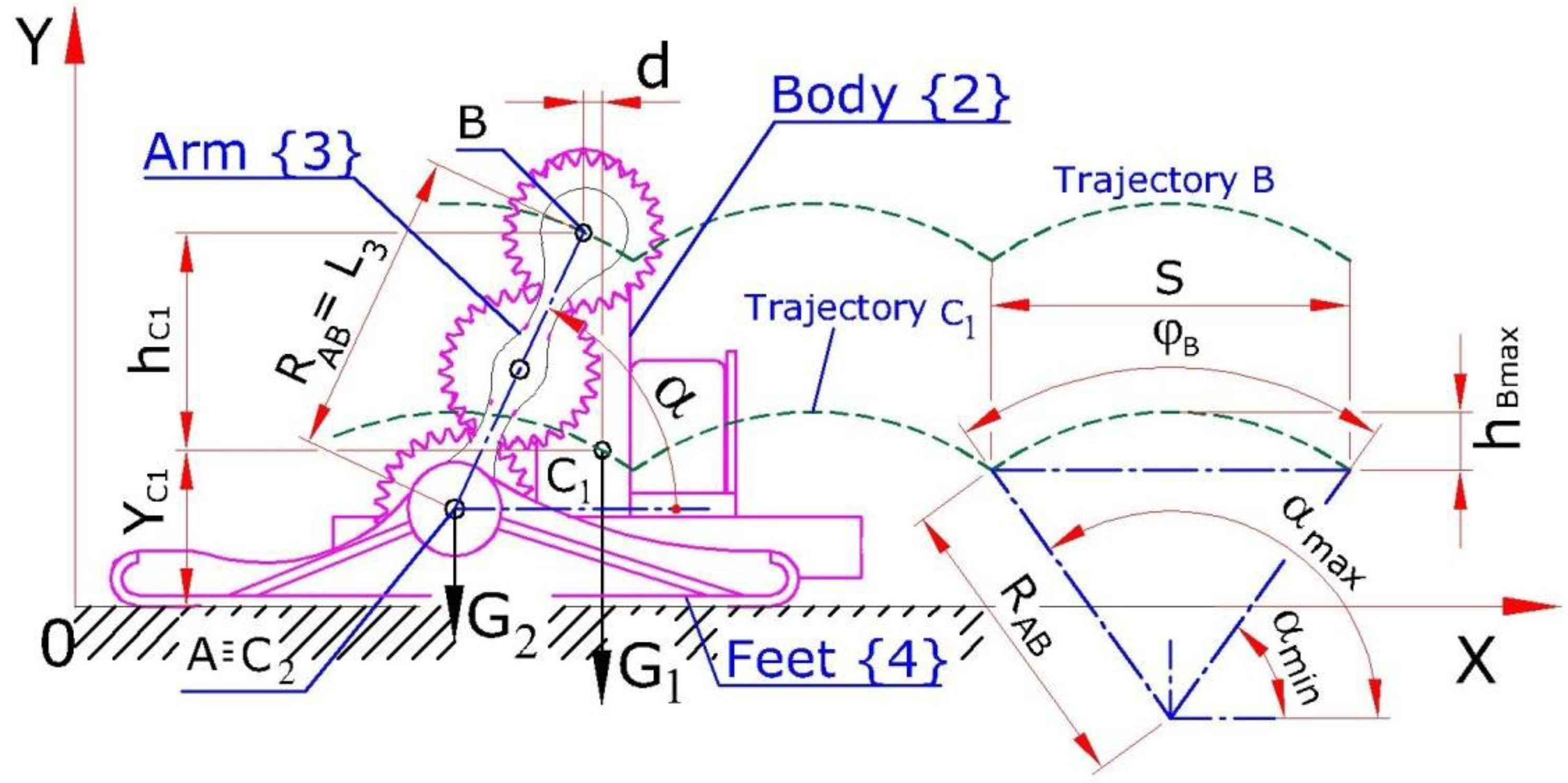
First phase—the support are the two feet {4}. Then the arm {3} is rotated at an angle $ϕ_{B} = α_{max} - α_{min}$ , where $α_{min} < α (t) < α_{max}$ (Figure 2). The body moves forward and all of its points move along parallel trajectories—arcs of a circle with a radius $R_{A B} = \bar{A B} = L_{3}$ . Thanks to the friction forces between the feet and the terrain, the robot moves one step S further. The instant center of rotation of the arm AB is at point A.

Figure 2.

Phase of support feet and geometric parameters.

It is assumed that during this phase, the mass m ₁ of the robot without the feet and the arms AB is concentrated in point C ₁. This point is displaced (at a distance d) from the axis of rotation B due to the large mass of the battery. Point C ₁ is as low as the design constraints allow, in order to increase the robot’s stability.

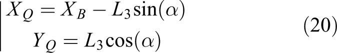
The distance the robot travels is determined by Figure 2 (trajectories C ₁ and B)

X_{C_{1}} = X_{B} + d = X_{A} + L_{3} cos (α) + d

where X_A is the current coordinate of point A from the fixed foot, $α = α (t)$ is the current angle of rotation of link AB relative to the horizon. The lifting of the center of gravity C ₁ of the body is

Y_{C_{1}} = Y_{B} - h_{C_{1}} = Y_{A} + L_{3} sin (α) - h_{C_{1}}

where $h_{C_{1}}$ is the vertical distance from axis B to point C ₁, which does not change when the robot moves. The movement is slow, so the inertial forces can be neglected. For the torques in axes A and B from the static laws can be written

M_{A_{1}} = [L_{3} cos (α) + d] G_{1}

M_{B_{1}} = d \cdot G_{1}

where $G_{1} = m_{1} g$ is the weight of the robot without the feet and arms AB, g is the Earth’s gravitational acceleration.

If (1) and (2) are differentiated are obtained the projections of the speed of the robot’s body during phase 1

| \begin{array}{l} V_{x} = {\dot{X}}_{C_{1}} = \dot{α} L_{3} sin (α) = ω L_{3} sin (α) \\ V_{y} = {\dot{Y}}_{C_{1}} = - \dot{α} L_{3} cos (α) = - ω L_{3} cos (α) \end{array}

where $ω = \frac{d α}{d t}$ is the angular velocity of the arm AB and it is set by the controllable motor {7} (Figure 1). The magnitude of the velocity is $V = \sqrt{V_{x}^{2} + V_{y}^{2}} = ω L_{3}$ , and its direction is along the tangent of the trajectory. When the body reaches the ground, it stops moving and a second phase begins. At higher velocities, an impact stress occurs in the transition between the phases.

Second phase —robot is standing on the circular base {1}. During this phase, the body {2} is stationary and only the arms {3} and feet {4} move. The mass m ₂ of the feet and the arms is considerably smaller than that of the robot’s body. It is assumed that it is concentrated in a point $C_{2} \equiv A$ , which is in the axis of rotation between the feet {4} and arms {3}. The arm revolves again, but this time its center of rotation is in point B. It rotates at an angle $ϕ_{S} = 2 π - ϕ_{B}$ . The feet move progressively and all their points describe arcs of a circle with radius $R_{A B} = L_{3}$ . The law of motion for C ₂ is obtained with similar reasoning as in phase 1. This movement does not lead to displacement of the robot, so it is not examined in detail. The torques in axes A and B in this phase of the motion are

M_{A_{2}} = 0 \cdot G_{2} = 0

M_{B_{2}} = [L_{3} cos (α)] G_{2}

$G_{2} = m_{2} g$ is the weight of the feet. From equations (3) to (7) and the big difference between G ₁ and G ₂, it is noticed that the loading in the shafts A and B is cyclic, with the shaft A being more loaded. The velocities of the feet can be determined from (5), taking into account the range of change of angle α for this phase. The phase ends when the feet make contact with the ground. At a constant angular velocity, impact loads at this phase are smaller than the first phase, because of the smaller moving mass m ₂. equations (3), (4), (6), and (7) do not take into account the impact loads during the transition between the two phases.

Geometric proportions of the links of the robot

This chapter addresses the problems associated with optimal proportions of the basic dimensions of the robot and minimizing energy losses during movement. Proportions are determined in which movement by walking is possible, the robot has a maximum step length and can attack an obstacle with maximum height.

In Figure 3 are presented the basic dimensions of the 3-D printed prototype. Five lengths ( $L_{1}, L_{2}, L_{3}, L_{4}, L_{5}$ ; Figure 3) and their proportions determine the qualities of the robot and its capability to walk and overcome obstacles. Obviously, the larger the model, the higher the obstacles that it can overcome. Therefore, the height of the obstacle h_o should be compared with the height—H_R and the length—B_R of the robot. Thus can be compared objectively different designs of one robot, and even a variety of different robots.

Figure 3.

Basic dimensions of the 3-D printed prototype.

As a generalized measure, is introduced a dimensionless index $K_{r o}$ , to compare a robot with the height of an obstacle—h_o , that it overtakes

K_{r o} = \frac{h_{o}}{\sqrt{H_{R} B_{R}}}

Thus, the index is typically in the range of $0 < K_{r o} < 1$ , and values above 1 would result in climbing and jumping robots.

Walking is possible only for a certain area of the robot’s dimensions— $L_{2}, L_{3}, L_{4}$ . It is necessary for the feet and the body to reach the ground. This condition is represented by the system of inequalities

| \begin{matrix} L_{2} \leq L_{3} + L_{4} \\ L_{4} \leq L_{2} + L_{3} \end{matrix}

Dimensions L ₁ and L ₅ are important for increasing the robot’s stability, but their excessive increase reduces the maneuverability of the robot and increases its overall dimensions.

From Figure 4 can be determined the step S, at which the robot moves

Figure 4.

Scheme for determining the geometric parameters for walking on flat terrain.

S = 2 \sqrt{L_{3}^{2} - {(L_{2} - L_{4})}^{2}}

Maximum lift height of the body $h_{B_{max}}$

h_{B_{max}} = L_{3} - L_{2} + L_{4}

Maximum lift height of the feet $h_{S_{max}}$

h_{S_{max}} = L_{2} + L_{3} - L_{4}

Angle $φ_{B}$ at which the arms are rotated during the phase of stationary feet

φ_{B} = 2 arctan (\frac{S}{2 (L_{2} - L_{4})})

and the angle $φ_{s}$ at which the arm is rotated during the phase of stationary base is $φ_{s} = 2 π - φ_{B}$ . From Figures 3 and 4, it can be determined that when attacking an obstacle with a height h_o with the robot’s body, in order to step on, it is necessary that $h_{o} < h_{B_{max}}$ , and in the case when attacking with the feet the condition is $h_{o} < h_{S_{max}}$ .

The dimension L ₄ cannot be less than the radius of the gear. L ₃ is also dependent on the parameters of the gear mechanism. These two parameters are determined from the mechanical design and can be changed in some way. If the lengths L ₃and L ₄ (constants) are known, after differentiating (10) in respect to L ₂ it is obtained

\frac{d S}{d L_{2}} = - \frac{2 (L_{2} - L_{4})}{\sqrt{L_{3}^{2} - L_{2}^{2} + 2 L_{4} L_{2} + L_{4}^{2}}}, L_{3}^{2} - L_{2}^{2} + 2 L_{4} L_{2} + L_{4}^{2} > 0

which shows that when $L_{2} = L_{4}$ , the function has an extreme, in this case it is a maximum (Figure 5).

Figure 5.

Change in the step S when changing L ₂.

This corresponds to the largest step $S_{max} = 2 L_{3}$ , the angle $ϕ_{B} = ϕ_{S} = π$ and $h_{B_{max}} = h_{S_{max}}$ . In this case, the robot moves at a maximum speed. An example of the variation of $S (L_{2})$ , when $L_{3} = 55 (mm)$ and $L_{4} = 17 (mm)$ , is given in Figure 5. The allowable area for variation of L ₂ is determined by (9) and is $0 < L_{2} < L_{3} + L_{4} = 72 (mm)$ .

Unlike wheeled robots, movement by walking has the disadvantage of losing a significant amount of energy to lift the legs and, in some cases, the body. This calls for a solution to minimize these losses. Since the body has a mass m ₁, significantly greater than m ₂, it is preferable to have less lift of the body than the feet— $h_{B_{max}} < h_{S_{max}}$ , which means movement with smaller steps but also better energy distribution during the two phases of walking. A reasonable compromise is sought between the lifting height of the body $h_{B_{max}}$ and the length of the step S. The idea is to equalize (equation (17)) the potential energies of the robot from the two phases (equations (15) and (16)) of walking on flatter terrain, in order to determine the appropriate dimensions in search of this compromise. Equalization of energies also indirectly results in a more favorable loading on the elements of the structure. Impact loads on flat terrain decrease because the vertical component of the velocity V_y is reduced, equation (5), see Figure 4.

The potential energy $E_{p_{1}}$ that is overcome by the motor when lifting the body is

E_{p_{1}} = m_{1} g h_{B_{max}}

and the energy during the phase of stationary body is

E_{p_{2}} = m_{2} g h_{S_{max}}

The equalized energies are as follows

E_{p_{1}} = E_{p_{2}} \Rightarrow m_{1} g h_{1} = m_{2} g h_{2}

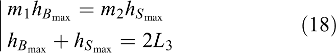
From (17) and geometrical considerations from Figure 4 $(h_{B_{max}} + h_{S_{max}} = 2 L_{3})$ , the following system is obtained

| \begin{array}{l} m_{1} h_{B_{max}} = m_{2} h_{S_{max}} \\ h_{B_{max}} + h_{S_{max}} = 2 L_{3} \end{array}

From (18), the height at which the body is lifted when the maximum potential energies, for the two phases are equalized, is as follows

h_{B_{max}} = \frac{2 L_{3} m_{2}}{(m_{1} + m_{2})}

The weights of the robot’s components are $m_{1} = 245 (g)$ and $m_{2} = 30 (g)$ . For the specific example from (19) is obtained $h_{B_{max}} = 12 (mm)$ . At $L_{3} = 55 (mm)$ , this corresponds to point R from the graph in Figure 5. Such a ratio between body lift height $h_{B_{max}}$ , feet lift height $h_{S_{max}}$ , and step S is embedded in the robot’s design and corresponds to the dimensions given in Figure 3. This energy-equalizing approach leads to the advantage of the feet being lifted at a significantly higher height $h_{S_{max}}$ than the heavy base. As a result, the robot can attack and overcome high obstacles with the feet. Such optimization of the dimensions of the robot also improves the dimensionless coefficient K_ro (8), because by preserving the size of the robot the possibility of overcoming a higher obstacle $h_{0} < h_{S_{max}}$ is increased.

Overcoming an obstacle

In this chapter is described the overcoming of an obstacle by the robot through analyzing trajectories of points from the robot and the alteration of the instantaneous center of velocities of the arm L₃ . The aim is to distinguish between different stages of movement and to determine the nature of the change of the instantaneous center of velocities.

Small obstacles with height $h_{0} < h_{B_{max}}$ are overcome easily. When attacking an obstacle with $h_{0} \geq h_{B_{max}}$ with the robot’s body, it cannot be overcome immediately. A process of passive adaptation of the robot with respect to the obstacle is observed, in which it “prepares to attack” with the feet. When the robot moves on flat terrain and a smooth vertical obstacle, the robot’s body slides along the vertical section (parallel to the Y axis) of the obstacle, the feet slide parallel to the X axis (Figure 6), and the arm AB performs a planar motion. With respect to the absolute coordinate system [O,X,Y], the coordinates of point Q—the instantaneous center of velocities for the arm (AB), can be defined as a function of the angle a(t) defined by the motor R2

Figure 6.

Instantaneous velocity center and adaptive movements in case of collision between the robot’s body and the obstacle.

| \begin{matrix} X_{Q} = X_{B} - L_{3} sin (α) \\ Y_{Q} = L_{3} cos (α) \end{matrix}

The instantaneous velocity center of the arm jumps from point A ₀ to point Q ₁ and starts to move along an arc of a circle (Figure 6). The equation of this circle with radius L ₃ and center $C_{Q} [- X_{B}, 0]$ is derived from (20), excluding the angle α, and is

{(X_{Q} + X_{B})}^{2} + Y_{Q}^{2} = L_{3}^{2}

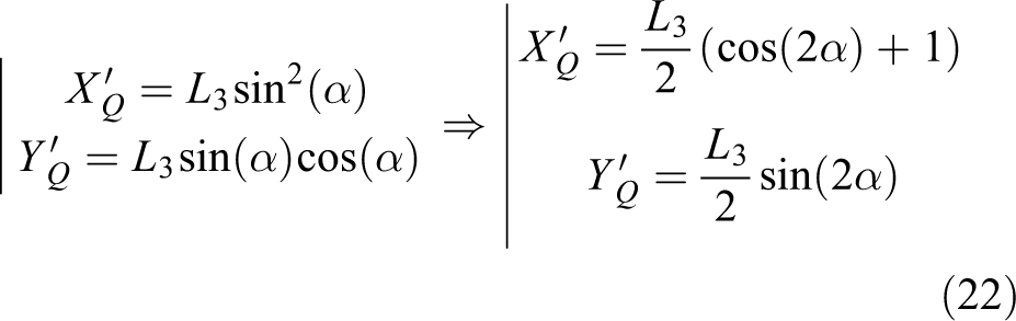
The relative instantaneous velocity center relative to the coordinate system $[A_{0}, X^{'}, Y^{'}]$ , and connected to the arm AB, is defined by the system of equations

| \begin{matrix} X_{Q}^{'} = L_{3} {sin}^{2} (α) \\ Y_{Q}^{'} = L_{3} sin (α) cos (α) \end{matrix} \Rightarrow | \begin{matrix} X_{Q}^{'} = \frac{L_{3}}{2} (cos (2 α) + 1) \\ Y_{Q}^{'} = \frac{L_{3}}{2} sin (2 α) \end{matrix}

The relative trajectory of the instantaneous velocity center is also an arc of a circle, and its equation is derived from (22) after excluding α

{(X_{Q}^{'} - \frac{L_{3}}{2})}^{2} + {(Y_{Q}^{'})}^{2} = {(\frac{L_{3}}{2})}^{2}

In Figure 6, the arc of the red circle is the trajectory (TMCa) relative to the absolute coordinate system OXY, and the blue arc is the trajectory (TMCr) in respect to the relative (movable) coordinate system associated with the arm AB. In this case, the robot’s body and feet are moving along axes X and Y, respectively, and the arms perform a planer motion. After the body touches the horizontal terrain, the instantaneous velocity center changes again and jumps to a point $B_{1}^{′}$ .

The case where the robot attacks the obstacle with the feet is more favorable. If the height of the obstacle h ₀ is less than the height $h_{S_{max}}$ at which the feet can be lifted, three scenarios are possible: climbing the obstacle; loss of stability—the robot rolls over; or multiple slippage, where the obstacle cannot be overcome. From the point of view of kinematics and determination of the instant center of rotation, five different stages of climbing the obstacle are of interest.

Stage 1. Overcoming an obstacle begins with the feet touching the obstacle and lifting the robot (Figure 7). In this case, the robot’s base {1} is in contact with the ground, and the feet {4} with the obstacle. The movement of the robot is possible only if there is slippage between the base {1} and the ground and/or the slippage between the feet {4} and the obstacle. The distance L ₀ is changing. All links of the robot perform planar motion.

Stage 2. After rotation of the arm {3}, a stage 2 is reached where the feet {4} are in contact simultaneously with the ground and the obstacle. Here the feet are stationary, the arm {3} rotates, and the body moves forward. The distance L ₀ does not change. The instant center of rotation of the arm {3} is at point A. At very high obstacles, it is possible to get the entire robot slipping.

Stage 3. Arm {3} continues to rotate until the base {1} reaches the obstacle. The base is in contact with the obstacle, and the feet {4} with the ground. The situation is similar to stage 1. The robot performs a planar motion and there is slippage between the feet, the base, the ground, and the obstacle. The distance L ₀ is changing.

Stage 4. It is reached a stage where the base {1} is in contact with both the obstacle and the ground simultaneously. The base is stationary and the arm {3} rotates with a center of rotation at point B. The feet {4} move progressively.

Stage 5. Depending on the height of the obstacle, the shape and materials of the base, the masses of the links and the feet, a stage can be reached in which the robot rotates around the edge of the obstacle at point C. The center of rotation of the base is at point C, and the arm and the feet perform a planar motion. The robot overcomes the obstacle. When descending, the robot goes through similar stages of motion.

Figure 7.

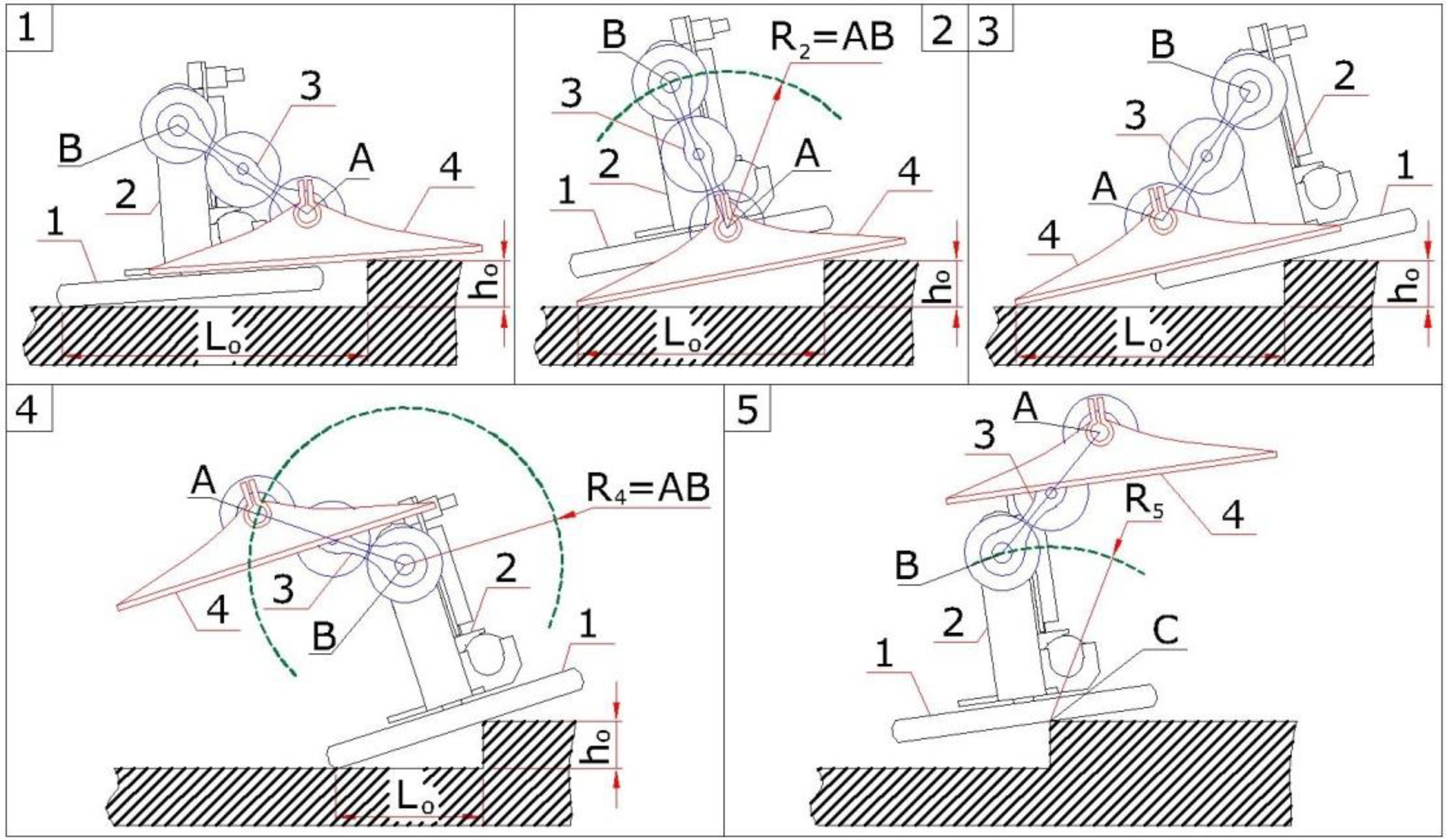
Five consecutive stages when climbing an obstacle.

Simulation of overcoming an obstacle

Description of the simulation

The purpose of the simulation is to generally identify the behavior of the robot when moving in a complex environment as well as the nature of the load on its main components. This will help in finding the optimal design and control strategies.

With the help of specialized software—MSC.visualNastran 4D—was made a simulation of the robot’s movements when overcoming an obstacle. It is developed a 3-D model of the robot with a round smooth base and flat feet. The angular velocity of the drive shaft (8) (Figure 1) is determined using the catalogue data of the used GM22 gearmotor with gear ratio i = 298 and the gear ratio of the gear mechanism i = 4. The resulting angular velocity 60 (°/s) is set as the velocity constant of the virtual motor. The toothed gears are modeled in the simulation with the corresponding constraints in such a way that the feet maintain a constant orientation relative to the base. Collisions between the robot, the ground, and the obstacle are taken into account. The restitution and friction coefficients are respectively 0.2 and 0.1. The simulation uses the integration method of Kutta-Merson with a variable integration step. The obstacle is modeled as a parallelepiped with a height of 10 (mm) and a length of 150 (mm). The simulation is done for 30 (s), with the robot climbing the obstacle, making two steps on it and descending it.

Results from the simulation

In Figure 8 are presented the simulation results. Given are graphs for the change of the horizontal displacement and horizontal velocity of the robot’s body, as well as the load (torque) of shaft {8}, which drives the walking mechanism.

Figure 8.

Results from the simulation of overcoming an obstacle.

Position 1 corresponds to the movement of the robot’s feet before reaching the obstacle.

In position 2, there is contact between the feet and the obstacle which corresponds to stage 1—here is observed slippage of the robot in the negative direction, as well as an abrupt change in the speed and torque. In this position, there is a maximum load on the motor and on the components of the robot.

Position 3 corresponds to stage 2—the robot’s body moves smoothly forward, the horizontal velocity changes smoothly going through the maximum and then decreasing. Change in loading of the motor is observed from positive to negative.

Position 4 corresponds to stage 3 when the body comes into contact with the obstacle—a negative slip begins, the velocity changes abruptly almost to zero and there is a jump in the loading of the motor.

Position 5 corresponds to stage 4—it is observed negative slippage, velocity close to zero and smooth change in the loading of the motor.

Position 6—the feet come into contact with the obstacle (phase 1), slippage and high torque values.

Position 7—corresponds to phase 2, and then to stage 5, positive displacement of the body, abrupt change in velocity and torque. The robot stands horizontally on the obstacle. It has climbed on the obstacle.

Position 8—the robot’s body is on the obstacle. Positions 9 and 10 correspond to a supporting body and supporting feet when moving on flat terrain. It is observed a non-slip movement and an abrupt change in velocity and torque when the support changes.

Position 11—the robot loses stability and begins to descent the obstacle. The velocity increases to the maximum before establishing contact with the ground. There is slippage in the positive direction.

Position 12—impact load on the robot, the velocity becomes zero.

Position 13—the feet touch the ground and begin a movement similar to stage 4, but on a slope.

Position 14 corresponds to supporting feet and position 15 to a supporting body. The obstacle is overcome.

From the simulation, it is concluded that slipping and impact loading are the most significant problems when overcoming an obstacle. The behavior of the robot corresponds to the theoretically described phases of motion.

Experiment

Experimental setup

Experiments are carried out to determine the trajectories of characteristic points from the robot’s links during its movement. Points A and B from the robot arm {3} are highlighted in a contrasting color to distinguish them from the other elements. The camera is stationary and is positioned perpendicular to the movement of the robot (Figure 9).

The following sequence is used to construct the instant centers of rotation of the arm {3}:

Figure 9.

(a) Experimental setup for determination trajectories when overcoming an obstacle. (b) Instantaneous center of velocity Q_i .

Capture the motion with a video camera.

A sequence of frames is generated from the resulting video.

Vector information about the coordinates of the highlighted points is obtained for each frame. In this case—the trajectories of points A and B from the arm {3}.

The centroid is constructed by connecting every two consecutive adjacent points A_i and A_i+1 with a segment. At a sufficient number of points, these segments are close to the tangent of the trajectory at this point. It is then constructed a perpendicular to the segments A_iA_i+1 , as well as to B_iB_i+1 , so that the lines pass through the points A_i and B_i , respectively. The intersection point Q_i of these lines is the instantaneous center of rotation. Points Q_i are connected to obtain the centroid. See Figure 10(b). When segments $\bar{A_{i} Q_{i}}$ and $\bar{B_{i} Q_{i}}$ are parallel (or close to parallel) and Q_i is at infinity then the link performs instantaneous translation. In the case when $\bar{A_{i} Q_{i}}$ and $\bar{B_{i} Q_{i}}$ are coinciding, there is not enough information to determine the instantaneous velocity center because the velocities of the points A_i and B_i are not known.

Figure 10.

(a) Trajectories of points A and B and (b) intersection points Q_i when attacking the obstacle with the base.

Using the proposed algorithm, the absolute instant centers of rotation are determined when climbing an obstacle. The camera that is used shoots at 25 frames per second. Two experiments are conducted: when the robot attacks the obstacle with its body (passive adaptation); and with its feet. The obstacle is 0.02 (m) high and has a horizontal and vertical sections.

A maximum height that a robot with given parameters can overcome is sought by using a 3-D printed model. Experiments are carried out with two variants of the robot’s base and feet: the first one from polylactic acid (PLA) only and for the second one is added a thin pad (the dimensions of the feet and the base do not change) from FilaFlex, rubber-like material.

Results from the experiment

From each frame is taken a pair of points corresponding to the position of points A and point B from link {3}. A graph with the trajectories of motion during passive adaptation to an obstacle is given in Figure 10(a). A sequence of points (frames) from 1 to 34 is presented. The trajectories of points A and B are denoted with a and b, respectively (Figure 10(a)). R ≈ 0.055 (m) is the radius of arcs approximating the trajectory of points A and B. The instant center of rotation of the link {3} is given in Figure 10(b). equation (21) determines the theoretical trajectory of motion of the instantaneous velocity center in case of contact with the obstacle and adaptive movements of the robot. The experimental results in this case are presented on Figure 10(b). Points 1–18 correspond to the movement of the robot’s body until it comes into contact with the obstacle. The instant centers—points 19–21 reflect the impact of the robot with the vertical section of the obstacle. It can be seen that the change in the instantaneous velocity center is abrupt and does not correspond to the theoretical one derived from equation (21), because the impact loads and the friction between the components are not taken into account. There follows a relatively smooth sliding of the body and the robot’s feet—points 22–25, which can be approximated by an arc of circle. At this point, there is a correlation between the theoretical trajectory and the experimental. The maximum deviation of these points of the theoretical arc is less than 1.6 (mm)). Follows a jump across points 26 and 27, then the stage of attacking the obstacle with the feet begins.

In Figure 11 is presented a graph with the trajectories of points A and B as well as the instant centers of rotation when climbing an obstacle.

Figure 11.

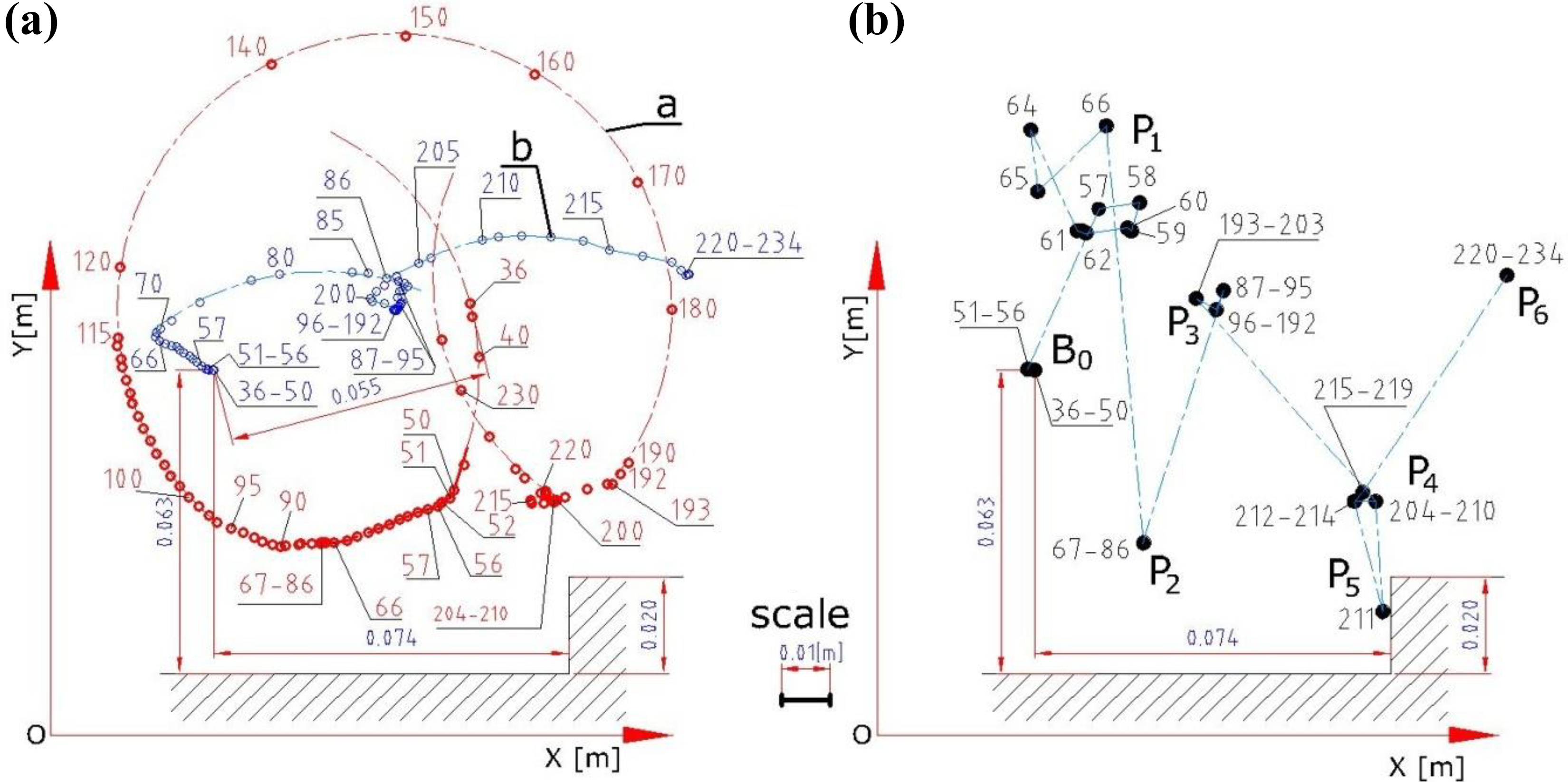
(a) Trajectories of points A and B and (b) intersection points Q_i when climbing an obstacle.

In Figure 11(a) are presented the trajectories of points A and B, and in Figure 11(b) the instantaneous centers of velocities obtained using the proposed algorithm. The dashed line in Figure 11(b) shows abrupt displacement of the instantaneous center of velocities. The graphs are obtained by using feet and base from PLA material only.

When the robot overcomes an obstacle, attacking it with its feet (Figure 11), the trajectories of points A and B are complex. The moment of contact between the feet and the obstacle occurs in frame (point) 51. After minor slippage of the center of velocity—51–56 (point B ₀) about 1.5 (mm), the instantaneous center of velocity abruptly changes to 57 and moves in a cluster P ₁ of points 57–66, during this time the robot slips in respect to the terrain and the obstacle. The feet touch the ground, the robot starts moving with fixed feet and its body describes a trajectory very close to an arc of a circle. This corresponds to P ₂—points 66–86 for the instantaneous centers of velocities. There follows a jump (contact of the base with the obstacle) to cluster P₃ —points 87–203. In this period (P ₃), the robot’s feet move and the body slides. (The diameter of cluster P ₃ is approximately 6 (mm).) There follows a jump-like displacement of the center of rotation into P ₄ and again the robot’s body moves along a trajectory close to an arc of a circle. (The diameter of cluster P ₄ is approximately 5 (mm).) For a very short time, just one frame, the instantaneous center of velocities passes through P ₅ and goes into cluster P ₆. This corresponds to rotation of the robot around point P ₅, very close to the edge of the obstacle which is key to overcoming it. Reaching P ₆ means that the obstacle has already been overcome.

The instantaneous center of rotation changes smoothly or abruptly. The abrupt change of the instantaneous center of rotation corresponds to an impact load on components of the robot. In the case of a smooth change of the center of rotation, there is slippage between the base and/or the feet with respect to the ground. Another situation that is observed corresponds to a fixed element (body or feet) from the robot with respect to the terrain. Such are, for example, positions 36–56 and 67–86 from Figure 11, where the instantaneous center of the velocities changes insignificantly.

The slippage in most cases is an undesirable effect because it reduces the speed of the robot and increases the energy loss. Experiments are carried out in which the robot and the obstacle are at a different starting distance. As a result, it is determined that there are situations where slippage leads to passive adaptation of the robot to the obstacle and facilitates climbing. The proposed algorithm can be applied to obstacles of varying heights and when moving on slopes, as well as when using different materials for the robot’s feet.

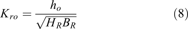
When the model has smooth feet and base made from PLA only, the maximum height it can overcome is 19 (mm), this corresponds to a factor of K_ro = 0.17 calculated from equation (8). The same model but with FilaFlex pads on the feet and the base overcomes a height of 37 (mm) which corresponds to K_ro = 0.34.

Conclusions

It is presented an original design of a walking robot with two degrees of freedom. The basic dimensions of the robot are analytically optimized to reduce energy losses when moving on flat terrain. Developed and produced is a 3-D printed model consistent with the obtained results.

Compared to the other walking robots that can overcome obstacles and climb stairs, the walking robot described in this study has a simple construction and only two controllable motors. It can overcome very high obstacles compared to its size, with a coefficient K_ro = 0.34. The robot is very maneuverable and can turn 360° around the vertical axis. The robot overcomes obstacles without the use of sensors and also maintains static stability during movement even without corrective control signals. It also adapts passively during overcoming an obstacle. Because of its simple design, the robot does not require complex control system which increases the reliability and robustness compared to other walking robots.

The stages of overcoming an obstacle are described. Simulation and experiments are carried out, which confirm the described robot behavior. The obtained results show the moments of impact loads and slippage of the robot.

It is proposed an algorithm for experimental determination of the instantaneous centers of rotation for different links of the robot, using sequential frames from a video. The obtained results are presented graphically. Based on the experiments, different phases of movement can be easily distinguished. Three types of movement are defined—motion with fixed feet with respect to the ground and the obstacle; movement in which there is slippage and a transient process during which the robot’s components are subjected to impact loads.

Experiments with various shapes and materials for the feet and base are carried out, which enhances its ability to overcome higher obstacles. The usage of FilaFlex material for the feet and the base reduces slippage which leads to the overcoming of significantly higher obstacles compared to the use of PLA only.

Part of the future work is the development of the sensor and control system of the robot is forthcoming. A specialized control algorithm is under development to reduce the dynamic loads described in another work.

Disadvantage of the design is the low speed of movement. With significantly high obstacles, the robot tries to overcome them, but there is a possibility of rolling over.

Footnotes

Declaration of conflicting interests

The author(s) declared no potential conflicts of interest with respect to the research, authorship, and/or publication of this article.

Funding

The author(s) disclosed receipt of the following financial support for the research, authorship, and/or publication of this article: These research findings are supported by the National Scientific Research Fund, Project N H17/10—12.12.2017.

ORCID iD

Ivan Chavdarov

References

Siegwart

Nourbakhsh

. Introduction to autonomous mobile robots, a Bradford book. Cambridge, MA; London, England: The MIT Press, 2004.

Akai

Kakigi

Yoneyama

, et al. Development of autonomous mobile robot that can navigate in rainy situations. J Rob Mech 2016; 28(4): 441–450.

Focchi

Orsolino

Camurri

, et al. Heuristic planning for rough terrain locomotion in presence of external disturbances and variable perception quality. Springer, Advances in Robotics Research: From Lab to Market 2018; 132: 165–209.

Sarmaha

Boruaha

Kalitaa

, et al. A bio-inspired implementation of walking and stair climbing on a quadruped robot. Procedia Comput Sci 2018; 143: 671–677.

Kanajar

Caldwell

Kormushev

. Climbing over large obstacles with a humanoid robot via multi-contact motion planning, 2017. In: 26th IEEE international symposium on robot and human interactive communication (RO-MAN), Lisbon, Portugal, August 28–September 1 2017, Portugal: IEEE.

Vázquez

Velasco-Villa

. Design and real-time control of a 4-DOF biped robot. Int J Adv Robot Syst 2013; 10(8): 1–11.

Ali

Shukor

Miskon

, et al. 3-D biped robot walking along slope with dual length linear inverted pendulum method (DLLIPM). Int J Adv Robot Syst 2013; 10(11): 1–12.

Omer

Hashimoto

Lim

, et al. Study of bipedal robot walking motion in low gravity: investigation and analysis. Int J Adv Robot Syst 2014; 11(9): 1–14.

Gao

Cui

Guo

, et al. Dynamics and stability analysis on stairs climbing of wheel–track mobile robot. Int J Adv Robot Syst 2017; 14(4): 1–13.

10.

Sudheer

Vijayakumar

Mohanda

. Stable gait synthesis and analysis of a 12-degree of freedom biped robot in sagittal and frontal planes. J Automat Mobile Robot Intell Syst 2012; 6(4): 36–44.

11.

Jeon

Yeo

Jeong

, et al. Bio-mimetic articulated mobile robot overcoming stairs by using a slinky moving mechanism. In: Proceedings of ICAD2009, The fifth international conference on axiomatic design, 25–27 March 2009, Campus de Caparica, pp. 173–179.

12.

Liu

Zang

Zhu

, et al. System overview and walking dynamics of a passive dynamic walking robot with flat feet. Adv Mech Eng 2015; 7(12): 1–10.

13.

Šimšaj

Kelemen

Virgala

, et al. Design of two legged robot. AM J Mech Eng 2013; 1(7): 355–360.

14.

Kwon

Park

. Kinesiology-based robot foot design for human-like walking. Int J Adv Robot Syst 2012; 9(6): 1–10.

15.

Kashiri

Abate

Abram

, et al. An overview on principles for energy efficient robot locomotion. Front Robot AI 2018; 5(129): 1–13.

16.

Huzaifa

Maguire

Viers

. Toward an expressive bipedal robot: variable gait synthesis and validation in a planar model. Int J Soc Robot 2019; 11: 1–13.

17.

Mummolo

Peng

Gonzalez

, et al. Contact dependent balance stability of walking robots. In: Proceedings of the ASME 2017 international design engineering technical conferences & computers and information in engineering conference, IDETC2017, Cleveland, OH, 6–9 August 2017, USA, pp. 1–7.

18.

Carpentier

Prete

Tonneau

, et al. Multicontact, locomotion of legged robots in complex environments—the Loco3D project. In: RSS workshop on challenges in dynamic legged locomotion, Boston, USA, July 2017, p. 3.

19.

Chavdarov

Tanev

Pavlov

. Walking robot. Patent application № 111362. Published summary—Billetin № 6, 30 June 2014, p. 11, in Bulgarian.

20.