Sage Journals: Discover world-class research

Abstract

In this article, a point-wise normal estimation network for three-dimensional point cloud data called NormNet is proposed. We propose the multiscale K-nearest neighbor convolution module for strengthened local feature extraction. With the multiscale K-nearest neighbor convolution module and PointNet-like architecture, we achieved a hybrid of three features: a global feature, a semantic feature from the segmentation network, and a local feature from the multiscale K-nearest neighbor convolution module. Those features, by mutually supporting each other, not only increase the normal estimation performance but also enable the estimation to be robust under severe noise perturbations or point deficiencies. The performance was validated in three different data sets: Synthetic CAD data (ModelNet), RGB-D sensor-based real 3D PCD (S3DIS), and LiDAR sensor-based real 3D PCD that we built and shared.

Keywords

Normal estimation 3-D deep learning 3-D sensor system 3-D indoor LiDAR data set robustness

Introduction

As the usage of point cloud data (PCD) continues to increase, it has been shown that not only PCD’s representation (x, y, z) but also PCD’s properties such as normal and intensity make significant contributions in various applications.^1
–3 Among those properties, this article focuses on the normal property of PCD, which is an orthogonal direction of a local planar patch constituted by multiple points.

Although there are a variety of conventional methods,^4

–7 their substantial layer is principle component analysis (PCA), which generates a local planar patch by sampling a few points in the nearest neighbor sense. As PCA is weak against noises, several variations that adaptively tune the algorithm parameters have been proposed.^8

–11 In the authors’ point of view, these approaches do not pinpoint the essential factors of normal estimation, as their performances drastically drop with increasing noise levels.

An alternative approach is to adopt the deep neural network designed for PCD, such as VoxNet,¹² ShapeNet,¹³ DeepPano,¹⁴ OctNet,¹⁵ and PointNet¹⁶, as a substantial layer. All of the above networks, except PointNet project 3-D PCD to low-dimensional primitives (such as volumetric representations,^12,13,17,18 octree representations,¹⁵ 2-D image projection representations,^14,19 and multiple data representations²⁰), and this projection, in return, makes point-wise normal estimation unavailable. In contrast, PointNet handles 3-D PCD as they are, and we adopt it as a substantial layer of our method.

However, PointNet only extracts local features using multilayer perceptron, which does not use neighboring information. In other words, PointNet has a deficiency in extracting local features. Considering this weakness of PointNet, several variations utilizing neighboring information have been proposed.^21,22

As a normal vector is a type of local information, we need to extract robust and informative local features. Therefore, we adopt the advantages of several methods^4,21
–23 to utilize neighboring information. The proposing network module, “multiscale K-nearest neighbor (K-NN) convolution module,” is shown in Figure 1. The multiscale K-NN convolution module is specially designed for normal estimation. In addition, we adopt the PointNet architecture as the basis model and utilize our proposing module into PointNet. The overall proposed network, NormNet, is shown in Figure 2. This network is trained by a 3-D PCD data set with labels of point-wise segmentation and normal. Here, note that each label of point-wise normal is not the ground truth but an estimation result by the automatic PCA method. This is a natural consequence of the huge amount of points (e.g. one of our data sets consists of 100 million points), and that is why we adopt automatic annotations at the sacrifice of accuracy.

Figure 1.

Multiscale K-NN convolution module. K-NN: K-nearest neighbor.

Figure 2.

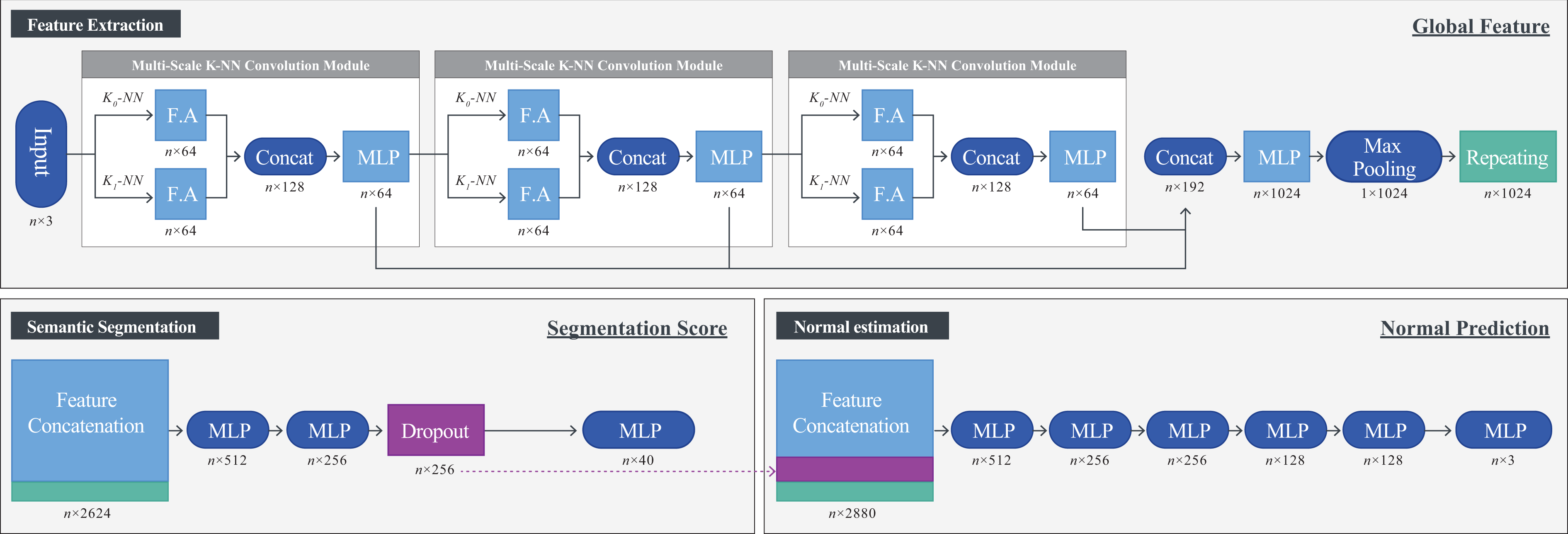
Architecture of the point-wise normal estimation network for 3-D PCD: NormNet. PCD: point cloud data.

The design principle of NormNet is to hybridize local, global, and semantic features simultaneously. The local feature corresponds to a point feature (sky-blue layers in Figure 2) of which the parameters are trained by estimated normal from the multiscale K-NN convolution module. The multiscale K-NN convolution module only use local feature like PCA methods, and it also contains weakness of the local feature that degrade performance near edges. We redeem this problem by using a global feature (the green layer in Figure 2). Also, the problem that local feature-based methods (PCA methods) are weak against noises can be handled by considering semantic information(such as floor and rounded ball) supported by a segmentation feature (the purple layer in Figure 2).

For comparison, the K-NN technique,⁴ PointNet,¹⁶ PointNet++,²¹ DGCNN,²² and PCPNet²⁴ were selected. The K-NN technique⁴ is the most popular one (Matlab, PCL libraries, etc.) among PCA-based methods. Comparing the basic PointNet architecture,¹⁶ PointNet++,²¹ DGCNN,²² and PCPNet²⁴ might show the novelty of the multiscale K-NN convolution module.

For training and testing, three data sets were used: a synthetic data set (ModelNet¹³), a RGB-D sensor-based real dat aset (S3DIS²⁵), and a LiDAR sensor-based real data set (PERL) that we built and shared on a web page.²⁶

The evaluation results show that the proposed method outperforms K-NN, PointNet, PointNet++, DGCNN, and PCPNet in ModelNet data set and tends to estimate more consistent normal in the S3DIS and PERL data sets. Furthermore, it appears that the proposed method captures more essential features than these methods, as its performance is far more robust.

The rest of this article is organized as follows. The proposed method is explained in the second section. Details of data sets are given in the third section. The evaluation results are analyzed in the fourth section, and the conclusion follows.

Methodology

Multiscale K-NN convolution module

Normals are local information, involving relations of neighboring features. Therefore, existing methods^4

–7 utilize K-NNs and PCA algorithm to compute relations of neighboring features. However, PointNet adopts basic multilayer perceptions for local feature extraction. In other words, PointNet only utilizes a point-wise feature as a local feature, so it does not contain information about the neighborhood. However, as a local feature, not only point-wise information but also neighbor information is very important for normal estimation.

To utilize relations of the neighboring information, we propose the multiscale K-NN convolution module which acts like the existing K-NN and PCA methods. The concepts are shown in Figure 1.

To implement our multiscale K-NN convolution module, we used pyramid pooling module,²³ multiscale grouping,²¹ and edgeConvolution²² as guidelines.

Our multiscale K-NN convolution module aggregates different scale of features, which is similar to PointNet++.²¹ We use multiscale feature aggregation because local features from different scale generate more robust and more informative than using only one scale.^21,23

For feature aggregation, there are many methods that can be used

​_{κ} x_{i}' = \sum_{j : (i, j) \in κ} θ_{j} f (x_{j})

​_{κ} x_{i}' = \underset{j : (i, j_{n}) \in κ}{avg} (f (x_{i}), f (x_{j_{0}}),..., f (x_{j_{k}}))

​_{κ} x_{i}' = max_{j : (i, j_{n}) \in κ} (f (x_{i}), f (x_{j_{0}}),..., f (x_{j_{k}}))

where x_i is a central pixel, x_j : (i, j) ∈ κ is a K-nearest neighbor points around it, θ_j are weights of each parameter, and function f indicates multilayer perceptrons.

Here, equation (1) denotes the weighted sum of features. Although PCD are unstructured and unordered data, the weighted sum causes difficulty in training, and not appropriated for a pointcloud data set. Equation (2) is a special case of equation (1), where every weight is equal to one divided by the number of points. Equations (2) and (3) are symmetric functions that resolve problems of pointcloud data set (unordered, unstructured). In particular, PointNet¹⁶ adopts equation (3) so as to extract global features.

In the proposed multiscale K-NN convolution module, we adopt edgeConvolution introduced in DGCNN²² for feature aggregation. The edgeConvolution is given by

​_{κ} x_{i}' = max_{j : (i, j_{n}) \in κ} (f (x_{i}), f (x_{j_{0}} - x_{i}),..., f (x_{j_{k}} - x_{i}))

Thus, given an F-dimensional point cloud with n points, edgeConvolution produces an F′-dimensional point cloud with the same number of points.

Combining multiscale feature aggregation and edgeConvolution as a local feature extraction, our multiscale K-NN convolution module is given by

x_{i}' = f (_{κ_{0}} x_{i}' \oplus_{κ_{1}} x_{i}')

where a function ⊕ denotes the feature concatenate operator.

The multiscale K-NN convolution module aggregates multiscale neighboring features, which enables it to utilize relations of the neighboring information.

Network architecture

The PointNet¹⁶ is an appropriate deep learning network for unordered, unstructured PCD. PointNet combining local feature (point feature) and global feature to predict point-wise classes. This approach is suitable for our problems, so we adopt PointNet as a substantial layer of our method. We integrate Pointnet with our proposed module (multiscale K-NN convolution module).

The proposed network, NormNet is shown in Figure 2, where “F.A” denotes the “feature aggregation” mentioned in the multiscale K-NN convolution module. Specifically, we adopted edgeConvolutions for feature aggregation. We adopt multilayer perceptrons with layer size 64 for the feature aggregation. “Conncat” denotes the feature concatenation that simply concatenates two or more features. “MLP” denotes the multilayer perceptron. “Repeating” denotes tiling the output of “Max Pooling” feature.

The network takes n-point clouds as input. This input passes into three multiscale K-NN convolution modules, one after another. This serially connected module extract local feature hierarchically. After this module, three outputs are concatenated from each multiscale K-NN convolution module, followed by the multilayer perception, and then the features are aggregated by max-pooling. We term this feature as a global feature same as in PointNet. The global feature contains global information of the input data. All of the sky-blue layers in feature extraction are termed local features.

In the semantic segmentation network, all of the local features and global features (sky-blue layers and green layer in Figure 2) are concatenated, followed by multilayer perceptrons and dropout layer, as shown in Figure 2. We term the output of dropout layer (purple layer in Figure 2) as a semantic feature because this feature contains semantic information of input.

Similar to the normal estimation network, concatenate not only all the local and global features but also the semantic feature, followed by multilayer perceptrons to predict normal.

Here, every layer used batch normalization with rectified linear unit (ReLu).

Objective function

In NormNet, a loss function is designed in a way that performs the original task of PointNet (semantic segmentation) as well as normal estimation. For the semantic segmentation, we adopted the cross entropy loss, which gives class-wise segmentation scores in K classes, defined as

L_{seg} (z, y) = - \frac{1}{N} \sum \sum_{i} y_{i} log (p_{i})

with $p_{i} = \frac{e^{z_{i}}}{\sum_{k} e^{z_{k}}}, for k = 1, ..., K$ . z_s and y_s are segmentation prediction and segmentation ground truth, respectively.

For the normal estimation, we designed a loss function of

\begin{array}{l} L_{normal} (z_{n}, y_{n}) = L_{ang} (z_{n}, y_{n}) + L_{1} (z_{n}, y_{n}) + L_{norm} (z_{n}) \end{array}

with $L_{ang} = \frac{1}{N} \sum | 1 - \frac{z_{n} \cdot y_{n}}{‖ z_{n} ‖ y_{n} ‖} |$ , $L_{1} = \frac{1}{N} \sum {| z_{n} - y_{n} |}_{1}$ , and $L_{norm} = \frac{1}{N} \sum {(1 - ‖ z_{n} ‖)}^{2}$ . z_n and y_n are normal prediction and target (ground truth) normal, respectively.

Combining the above two losses, our total loss for our network is as follows.

L_{total} = L_{seg} + L_{normal}

Now, let us describe the physical meaning of these loss functions. The first term L_ang contains cosine distance, which gives low values when the predictions are similar to the ground truth. However, as its derivative tends to drastically decrease from a tipping angle of 30°, an additional term that derives the loss to zero is needed. Thus, we add L ₁, the derivative of which is −1, from the tipping angle to zero. In addition, we adopt a normalization factor L_norm, so that multiple loss values can evenly contribute.

Data set

For the training and validation of networks, we made use of three data sets, including a synthetic CAD data set (ModelNet40¹³ shown in Figure 3), and a real 3-D PCD acquired by RGB-D sensor (S3DIS²⁵ shown in Figure 4). As there is no indoor data set from LiDAR sensor, which is as popular as RGB-D in the robotics field, we built our own data set called PErecptional Robotics Lab (PERL shown in Figure 5). All of these data sets can be downloaded from the web page²⁶ as used in this article.

Figure 3.

Sample images of synthetic data sets: ModelNet40, and generated Pointcloud..

Figure 4.

Sample image of RGB-D data set: Matterport 3-D scanner and S3DIS data set.

Figure 5.

Sample image of 3-D LiDAR data set: sensor system with two LiDARs (Velodyne VLP-16), 9-DoF IMU (3DM-GX3-45), and 360 Camera (Ladybug 5).

Synthetic data set: ModelNet40

ModelNet data set was introduced in 3-D ShapeNet,¹³ the purpose of which is 3-D shape recognition and reconstruction. This data set follows the standard CAD format and consists of edges and vertices. It contains 12,311 models with 40 labels.

However, as there is neither a point cloud nor its normal, we manipulated ModelNet in such a way that 4096 points are uniformly sampled from CAD model. The normals of each point were calculated by the cross product of edges of a face. As this is an ideal data set, we intentionally added Gaussian noise with its mean and standard deviation (σ) of 0 and 0–0.02, respectively. In addition, to minimize the effect of wide range of object’s size (from small chair to huge airplane), we normalized all objects’ size into a unit sphere.

RGB-D data set: S3DIS

The S3DIS data set was introduced by Armeni et al.,²⁵ the purpose of which is a point-wise semantic parsing of 3-D PCD. This data set was constructed using a Matterport scanner which is assembled of multiple RGB-D sensors. It consists of six subsets that cover 271 rooms with 13 categories.

For NormNet, we modified S3DIS in such a way that 4096 points were randomly sampled from a block. Here, a block covers 1 × 1 m², of which half overlaps to the previous block and the other half to the next one.

LiDAR data set: PERL

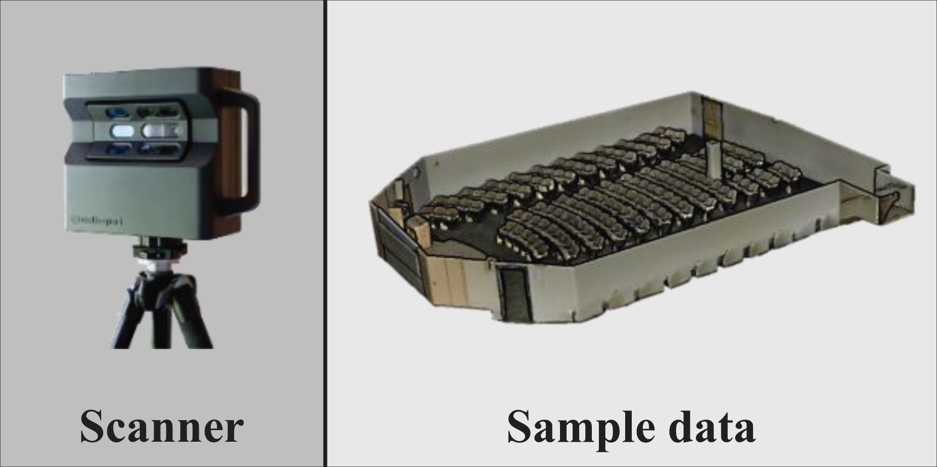
As there is no publicly available Indoor LiDAR PCD data set, we built our own using a sensor system, as shown in Figure 5. This system is composed of two LiDARs (Velodyne VLP-16), 9-DoF IMU (3DM-GX3-45), and 360 Camera (Ladybug 5).

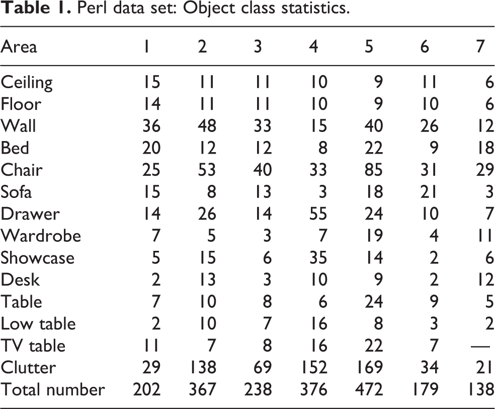
As our interest is objects, we set our target place to furniture exhibition shops. Using the sensor system, we scanned seven shops and conducted pose-optimization with our SLAM algorithm.²⁷ We manually segmented each object in 14 categories, the details of which are presented in Figure 6 and Table 1.

Figure 6.

Images of PERL data set: seven areas with 1972 obejcts in 14 categories.

Table 1.

Perl data set: Object class statistics.

Area	1	2	3	4	5	6	7
Ceiling	15	11	11	10	9	11	6
Floor	14	11	11	10	9	10	6
Wall	36	48	33	15	40	26	12
Bed	20	12	12	8	22	9	18
Chair	25	53	40	33	85	31	29
Sofa	15	8	13	3	18	21	3
Drawer	14	26	14	55	24	10	7
Wardrobe	7	5	3	7	19	4	11
Showcase	5	15	6	35	14	2	6
Desk	2	13	3	10	9	2	12
Table	7	10	8	6	24	9	5
Low table	2	10	7	16	8	3	2
TV table	11	7	8	16	22	7	—
Clutter	29	138	69	152	169	34	21
Total number	202	367	238	376	472	179	138

Experiments

For experiments, three sets of data are used: one synthetic and two real data sets. Considering that labeling point-wise ground truth cannot be realized for the real data set (due to huge amount of points), the synthetic and real data sets are in a complementary relationship as follows. Quantitative analyses can be conducted for the synthetic data (as there is the ground truth), while only qualitative interpretation is available for the real data. By contrast, the effects of the real noises cannot be evaluated for the synthetic data, while those with RGB-D and LiDAR sensors can be verified in the real S3DIS and PERL data set, respectively.

Synthetic data set: ModelNet experiments

In this section, we use K-NN method⁴ PCPNet,²⁴ PointNet,¹⁶ PointNet++,²¹ and DGCNN²² for comparisons. Here, the K-NN method⁴ and the PCPNet²⁴ only use local patches, which estimate normals without global information. However, PointNet,¹⁶ PointNet++²¹ and DGCNN²² can estimate normals with global information (including segmentation feature). To compare with the same conditions, we applied the same loss function and architecture, aside from the local feature extraction module. PointNet uses multilayer perceptions, PointNet++ uses multiscale grouping (MSG), and DGCNN uses edgeConvolutions for local feature extraction.

As the performance of the K-NN-based method depends on the value of k, the physical meaning of which is the number of points to use for local feature extraction, we first conducted a performance test for various k values, as shown in Figure 7. Here, the solid and dashed lines indicate percentages, the estimated angle errors of which are within 25° and 15° (‘accuracy #’ from now on) relative to the ground truth, respectively. Based on this test, k was set to be 27, where the accuracy 25° hits the maximum.

Figure 7.

Accuracy of K-NN as k value varies, where k = 27 shows the best performance. K-NN: K-nearest neighbor.

With these k values, accuracies for various angles (from 25° to 1°) were evaluated as in Table 2. Here, it can be noted that as the judging criteria become strict, NormNet outperforms the K-NN based method, PointNet, PointNet++, DGCNN, and PCPNet. This result is illustrated in Figure 8, which shows a relative accuracy enhancement of NormNet as the judging criteria become strict. Some experimental examples are shown in Figure 9.

Table 2.

ModelNet40 result: Percentage of points of which the estimated angle error is within a certain bound for K-NN, PCPNet, PointNet, PointNet++, DGCNN, and NormNet.

	Accuracy within degree (%)
	25°	20°	15°	10°	5°	3°	1°
K-NN method	74.40	70.61	65.29	57.06	41.43	31.77	21.39
PCPNet	88.71	86.65	83.57	78.11	64.73	51.14	18.30
NormNet (baseline)	87.26	85.57	83.34	79.61	70.56	63.78	54.87
PointNet	77.51	74.74	71.51	66.04	56.42	50.33	39.78
PointNet++	83.83	81.70	78.83	74.13	63.12	53.91	29.63
DGCNN	87.53	85.73	83.17	78.80	69.19	63.02	54.95
NormNet	89.45	87.92	85.84	82.19	73.23	66.56	57.65

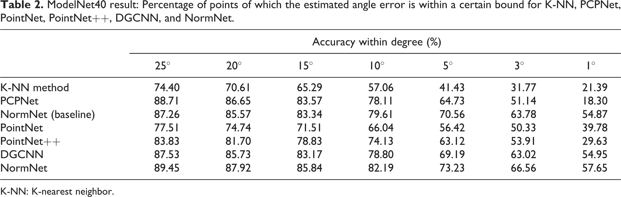
K-NN: K-nearest neighbor.

Figure 8.

Accuracy enhancements of PointNet (purple), PointNet++ (yellow), DGCNN (green), PCPNet (blue), and NormNet (red) relative to K-NN as degree of judging criteria decreases. K-NN: K-nearest neighbor.

Figure 9.

Point normals of ground truth (left), K-NN (center), and NormNet (right) for ModelNet40. Here, green, blue, and red arrows indicate that each normal estimation error is <15°, <25°, and >25°, respectively. K-NN: K-nearest neighbor.

Comparing NormNet with the K-NN-based method, the relative accuracy enhancement is drastic (Figure 8). This result is natural because the K-NN-based method only uses local patch (local information) for normal estimation. This means that K-NN-based methods do not consider the overall shape of features. As a result, point clouds on the edge or sharp inflection points estimate the normal smoothly. Also there exists various estimated normals despite point clouds on the same plane due to noises or effect of points on the neighbor planes. However, NormNet uses not only local feature but also global feature for prediction. As a result, point clouds on the edge or sharp inflection points estimate the normal sharply.

PCPNet also estimates normals without global information. PCPNet extracts local patches and estimates normal using learned features. However, PCPNet contains some problems. First, PCPNet is deeply based on PointNet network, which cannot estimate essential local features. This result is illustrated in Figure 8, which shows PCPNet shows similar accuracy in 25% but shows poor performances when judging criteria become strict. Second problem is computation complexity. PCPNet estimates normal by extracting local patches at every pointclouds, and this takes a lot of time. PCPNet takes 11,626 s for evaluating every ModelNet40 test data set. However NormNet only takes 502.53 s.

Comparing NormNet yield with PointNet, PointNet++, and DGCNN, NormNet estimates more accurate normals than these methods, as represented in Table 2. This result indicates that the multiscale K-NN convolution module captures more essential features than multilayer perceptron, multiscale grouping, and edgeConvolution.

We also evaluate effect of semantic features for normal estimation. We estimate normals using NormNet without segmentation feature. This result is shown in Table 2, under the name of NormNet (baseline). This result shows that segmentation features increase the accuracy about 2%.

Regarding the robustness, two realistic scenarios need to be considered. The first is to consider sensor noises as dynamic factor. By the term dynamic, we mean that even though one tunes a noise level after many trial and errors, it may vary with distance or as the surface materials of the target change. Thus, it needs to be considered that noise levels of training and testing data set could differ.

To test the robustness in this scenario, we first set a reasonable range of sensor noise from σ = 0.00 to σ = 0.02 by referring several research papers.^28
–30 We then trained PointNet, PointNet++, DGCNN, PCPNet, and NormNet for four cases(σ = 0.00, 0.004, 0.01, 0.02) and found the best k values for the K-NN-based method in each case as we did in Figure 7. After these preparations, we tested robustness against different noise levels as they vary in the reasonable range as in Figure 10.

Figure 10.

Accuracy of K-NN (black), PointNet (purple), PointNet++ (yellow), DGCNN (green), PCPNet (blue), and NormNe t(red) for their accuracy 25° (solid) and 15° (dashed) as test noise σ varies. Here, training noise σ was set to be 0.0, 0.004, 0.01, 0.02 for (a) to (d), respectively. K-NN: K-nearest neighbor.

Figure 10(a) is a result of training with zero noise. This result properly shows our intuition work. The NormNet’s graph is similar to the K-NN’s, which means that our multiscale K-NN module extract local features like the K-NN.

Figure 10(b) is a result of training noise σ = 0.004. Figure 10(b) shows that NormNet outperforms K-NN, PointNet, PointNet++, and PCPNet within the 4σ (4 times training noise), and DGCNN within the 3σ (3 times training noise). In other words, NormNet outperforms K-NN, PointNet, PointNet++, DGCNN, and PCPNet in the RGB-D sensor noise level.

Figure 10(c) and (d) shows the results of training noise σ = 0.01, 0.02, respectively. Figure 10(c) and (d) shows that NormNet outperforms not only K-NN but also PointNet, PointNet++, DGCNN, and PCPNet within the RGB-D sensor and LiDar noise level.

The second scenario is to consider that practical users tend to sample a part of PointCloud due to the huge amount of points. Thus it needs to be verified whether normal estimation methods still work well under this point deficiency. For this, for the same four σ and k values as before, accuracies were tested as the missing points increase, as shown in Figure 11. In this test, NormNet consistently works well with up to 85% missing points.

Figure 11.

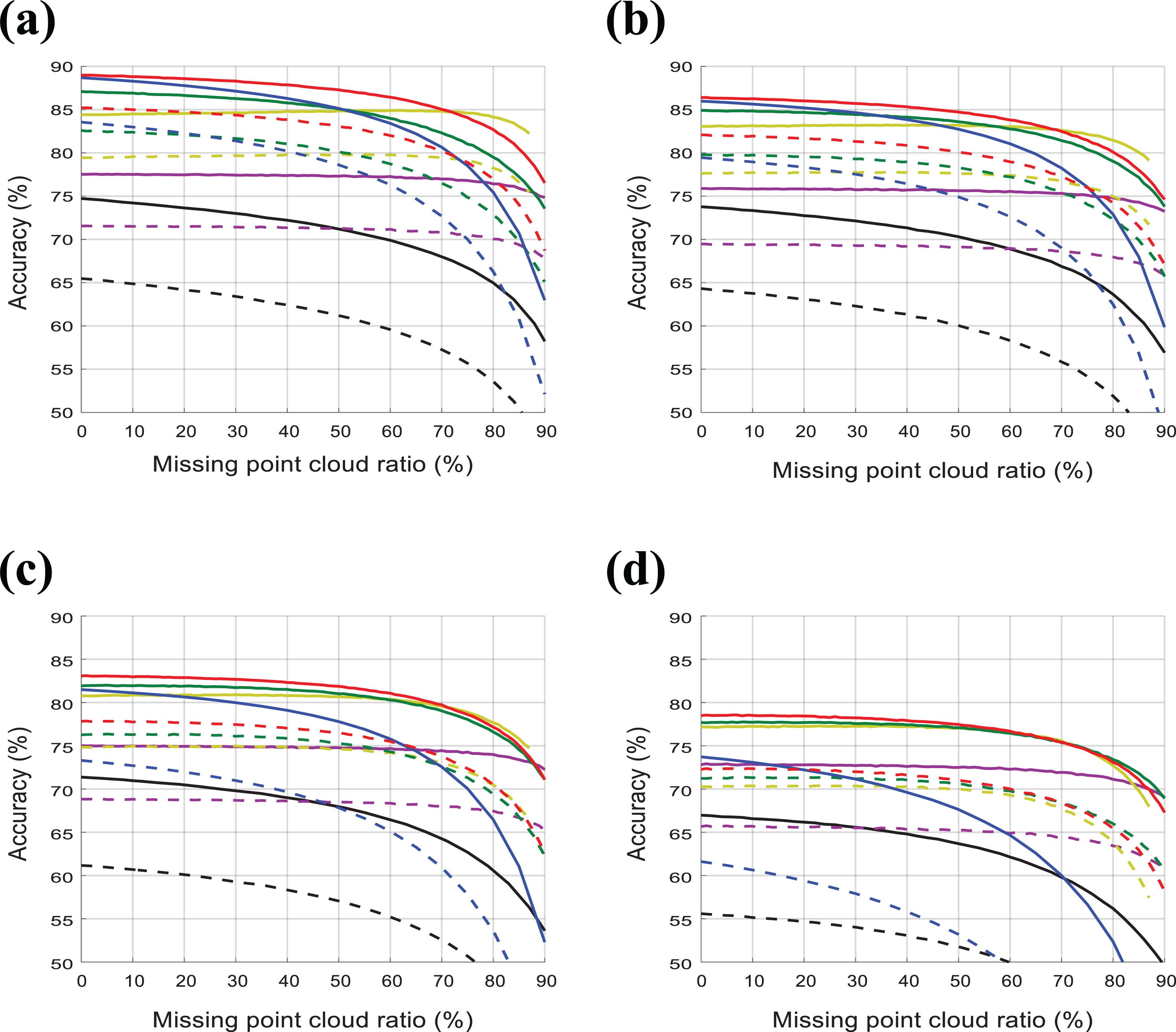
Accuracy of K-NN (black), PointNet (purple), PointNet++ (yellow), DGCNN (green), PCPNet(blue), and NormNet(red) for their accuracy 25° (solid) and 15° (dashed) as test PCD density varies. Here, training noise σ was set to be 0.0, 0.004, 0.01, 0.02 for (a) to (d), respectively. K-NN: K-nearest neighbor.

From this result, we carefully insist that the contributions of the global and the semantic feature are significant as the performances are still consistent in the ranges of up to 85%, where the contribution of local features mostly diminishes.

Real data sets: S3DIS and PERL experiments

For the real data set, we trained the proposed network with two kinds of annotations: point-wise segmentation and normals. Considering the ground truth of these, the segmentation can be manually labeled while that of the normal is beyond human’s labor (as there are billions of points). This indicates that a quantitative comparison can be applied for the segmentation and that we need to adopt a qualitative comparison for normals.

First, as the synthetic analysis in Table 2 shows segmentation features enhances the estimation of normal. Thus, we can implicitly insist that better segmentation yields better normal estimation. The segmentation results are presented in Table 3. Here, the S3DIS result is the mean of a threefold evaluation, as in the original paper, and the PERL result is the mean of a sevenfold evaluation with six areas for training and one area for testing.

Table 3.

S3DIS and PERL result: segmentation accuracy and mean Intersection over Union values for PointNet, PointNet++, DGCNN, and NormNet.

	S3DIS		PERL
	Overall Accuracy	mIoU	Overall Accuracy	mIoU
	(%)	(%)	(%)	(%)
PointNet	78.62	47.71	74.62	34.40
PointNet++	84.80	57.51	79.56	47.45
DGCNN	84.1	56.1	80.66	42.93
NormNet	84.48	57.06	80.86	43.94

mIoU: mean Intersection over Union; K-NN: K-nearest neighbor

Second, regarding the qualitative comparison for normals, we set the result of K-NN-based method as a pseudo-ground truth and trained each method using the same pseudo-ground truth. A qualitative approach that examines tendencies of irregular normals of which estimations from K-NN, PointNet, and NormNet are quite different is adopted. Examples are shown in Figures 12 and 13 for S3DIS and PERL data, respectively. Here, for places of which normals are evident, irregular normals are shown in red arrows. As it can be observed NormNet outperforms than K-NN and PointNet.

Figure 12.

Given S3DIS data set, point-wise normals were estimated using K-NN (top), PointNet (middle), and NormNet (bottom). Here, blue and red arrows indicate point normals within 25° and >25° differences between K-NN respective to NormNet, PointNet respective to K-NN and NormNet respective to K-NN estimations, respectively. Here, red arrows are shown on the surface of corridor (the first column), angled chair (the second column), shiny floor (the third column), rounded desk (the fourth column), and irregular objects (the fifth column). K-NN: K-nearest neighbor.

Figure 13.

Given PERL data set, point-wise normals were estimated using K-NN (top), PointNet (middle) and NormNet (bottom). Similar to the result of S3DIS, red arrows appear either on edges or irregular surfaces. K-NN: K-nearest neighbor.

We attribute the enhancement to three reasons. The first is that the global and semantic features correct locally distorted normal directions. The second is that the multiscale K-NN convolution module extracts essential local features well. The third is that the robustness against a wide range of noise levels enabled consistent estimation for carpets and floor (as shown in the second and fourth row from the top in Figure 12) and sharp edges (Note that time-of-flight sensors such as RGB-D sensor and LiDAR are sensitive on edges where reflection energies significantly drop due to light scatterings.).

Conclusions

This article proposed a NormNet which estimates surface normals. The NormNet not only successfully segments 3-D PCD (as does PointNet) but also accurately estimates normal direction better than the previous method K-NN.⁴ The key contributions are the design of local feature extraction module and the extraction of a surface normal in a hybrid way: global and semantic features from PointNet architecture and local feature from the proposed module, multiscale K-NN convolution module. Although analytic proof is not available due to the complex network structure, the experimental results implicitly support our claim that those three features mutually support each other. As a consequence, normal estimation became not only more accurate but also quite robust against noise perturbations or point deficiencies. In addition, the segmentation performance, which is the main role of PointNet, is increased. Finally, it is worth noting that we for the first time built and shared a LiDAR sensor-based 3D indoor PCD PERL data set.

Footnotes

Declaration of conflicting interests

The author(s) declared no potential conflicts of interest with respect to the research, authorship, and/or publication of this article.

Funding

The author(s) disclosed receipt of the following financial support for the research, authorship, and/or publication of this article: This work was supported by the Brain Korea 21 Plus Project in 2019, National Research Foundation of Korea (NRF) Grant (No. NRF-2011-0031648) funded by the Ministry of Science and ICT (MSIT), a Korean Evaluation Institute of Industrial Technology (KEIT) Grant (No. 10073166) funded by the Ministry of Trade, Industry and Energy(MOTIE), and a Grant (No. 19NSIP-B135746-03) from National Spatial Information Research Program (NSIP) funded by Ministry of Land, Infrastructure and Transport of Korean government.

ORCID iD

Janghun Hyeon

Weonsuk Lee

Joo Hyung Kim

References

Ikehata

Yang

Furukawa

. Structured indoor modeling. Proc IEEE Int Conf Com Vision 2015; 1323–1331.

Kazhdan

Hoppe

. Screened poisson surface reconstruction. ACM Trans Graph 2013; 32(3): 29.

Lafarge

Alliez

. Surface reconstruction through point set structuring. Comput Graphics Forum 2013; 32(2): 225–234.

Hoppe

DeRose

Duchamp

. Surface reconstruction from unorganized points. Assoc Comput Mach 1992; 26(2): 71–78.

Carr

Beatson

Cherrie

. Reconstruction and representation of 3D objects with radial basis functions. In: Proceedings of 28th annual conference on computer graphics and interactive techniques 2001, pp. 67–76. New York, USA: ACM.

Alexa

Behr

Cohen-Or

. Computing and rendering point set surfaces. IEEE Trans Visual Comput Graph 2003; 9(1): 3–15.

Mitra

Nguyen

. Estimating surface normals in noisy point cloud data. In: Proceedings of the 9th annual symposium on computational geometry, San Diego, California, USA, 08–10 June 2003, pp. 322–328. New York, USA: ACM.

Jones

Durand

Zwicker

. Normal improvement for point rendering. IEEE Comput Graph 2004; 24(4): 53–56.

Öztireli

Guennebaud

Gross

. Feature preserving point set surfaces based on non-linear kernel regression. Comput Graph Forum 2009; 28(2): 493–501.

10.

Schnabel

Klein

. Robust normal estimation for point clouds with sharp features. Comput Graph 2010; 34(2): 94–106.

11.

Huang

Zhang

. Consolidation of unorganized point clouds for surface reconstruction. ACM Trans Graph 2009; 28(5): 176.

12.

Maturana

Scherer

. Voxnet: a 3D convolutional neural network for real-time object recognition. In: Proceedings IEEE/RSJ international conference on intelligent robots and systems, 28 September – 2 October 2015, pp. 922–928. Hamburg, Germany: IEEE.

13.

Song

Khosla

. 3D ShapeNets: a deep representation for volumetric shapes. In: Proceedings of IEEE international conference on computer vision and pattern recognition, 7–12 June 2015, pp. 1912–1920, Boston, MA, USA: IEEE.

14.

Shi

Bai

Zhou

. Deeppano: deep panoramic representation for 3D shape recognition. IEEE Signal Proc Let 2015; 22(12): 2339–2343.

15.

Riegler

Ulusoys

Geiger

. Octnet: learning deep 3D representations at high resolutions. In: Proceedings of IEEE international conference on computer vision and pattern recognition, 2017, pp. 3577–3586.

16.

. PointNet: deep learning on point sets for 3D classification and segmentation. In: Proceedings of IEEE international conference on computer vision and pattern recognition, 2017, pp. 652–660.

17.

Sedaghat

Zolfaghari

Brox

. Orientation-boosted voxel nets for 3D object recognition. In: arXiv preprint arXiv:1604.03351, 2016.

18.

Brock

Lim

Ritchie

. Generative and discriminative voxel modeling with convolutional neural networks. In: arXiv preprint arXiv:1608.04236, 2016.

19.

Maji

Kalogerakis

. Multi-view convolutional neural networks for 3D shape recognition. In: Proceedings of the 2015 IEEE international conference on computer vision (ICCV), 7–13 December 2015, pp. 945–953. Washington, DC, USA: IEEE Computer Society.

20.

Hegde

Zadeh

. Fusionnet: 3D object classification using multiple data representations. In: arXiv preprint arXiv:1607.05695, 2016.

21.

. PointNet++: deep hierarchical feature learning on point sets in a metric space. In: Advances in Neural Information Processing Systems (NIPS), 2017, pp. 5099–5108.

22.

Wang

Sun

Liu

. Dynamic Graph CNN for learning on point clouds. CoRR 2018; abs/1801.07829.

23.

Zhao

Shi

. Pyramid scene parsing network. In: Proceedings of IEEE international conference on computer vision and pattern recognition, 2017, pp. 2881–2890.

24.

Guerrero

Kleiman

Ovsjanikov

. PCPNet learning local shape properties from raw point clouds. In: Computer Graphics Forum. Vol. 37. Wiley Online Library, 2018, pp. 75–85.

25.

Armeni

Sener

Zamir

. 3D semantic parsing of large-scale indoor spaces. In: Proceedings of IEEE international conference on computer vision and pattern recognition, 2016, pp. 1534–1543.

26.

PERL Dataset: 3D Indoor point cloud dataset, Velodyne VLP-16. http://sites.google.com/site/nakjudoh/normnet.htm. 2017.

27.

Lee

Ryu

Yeon

. Accurate continuous sweeping framework in indoor spaces with backpack sensor system for applications to 3-d mapping. IEEE Robotics and Automation Letters 2016; 1(1): 316–323.

28.

User’s manual and programming guide VLP-16. Morgan Hill, CA: Velodyne; 2017.

29.

Kang

Doh

. Full-DOF calibration of a rotating 2-D LIDAR With a simple plane measurement. IEEE Trans on Robotics 2016; 32(5): 1245–1263.

30.