
Abstract
The k-nearest neighborhoods (kNN) of feature points of complex surface model are usually isotropic, which may lead to sharp feature blurring during data processing, such as noise removal and surface reconstruction. To address this issue, a new method was proposed to search the anisotropic neighborhood for point cloud with sharp feature. Constructing KD tree and calculating kNN for point cloud data, the principal component analysis method was employed to detect feature points and estimate normal vectors of points. Moreover, improved bilateral normal filter was used to refine the normal vector of feature point to obtain more accurate normal vector. The isotropic kNN of feature point were segmented by mapping the kNN into Gaussian sphere to form different data-clusters, with the hierarchical clustering method used to separate the data in Gaussian sphere into different clusters. The optimal anisotropic neighborhoods of feature point corresponded to the cluster data with the maximum point number. To validate the effectiveness of our method, the anisotropic neighbors are applied to point data processing, such as normal estimation and point cloud denoising. Experimental results demonstrate that the proposed algorithm in the work is more time-consuming, but provides a more accurate result for point cloud processing by comparing with other kNN searching methods. The anisotropic neighborhood searched by our method can be used to normal estimation, denoising, surface fitting and reconstruction et al. for point cloud with sharp feature, and our method can provide more accurate result comparing with isotropic neighborhood.
Introduction
In the field of reverse engineering application, generally, two methods including contact and non-contact scanning devices are used to acquire 3D point cloud of objects, 1 but the collected data is 3D point cloud commonly. It can realize surface reconstruction and product remanufacturing by processing the point cloud. However, there is not any topological structure for scattered point cloud only containing 3D coordinate information.
Most point cloud processing methods depend on the neighborhood structure of point. Efficiency and accuracy of neighborhood searching method directly affect the speed and result of point cloud processing including normal estimation, 2 point cloud registration, 3 denoising 4 and surface reconstruction. 5 For example, estimating normal usually needs to search k nearest neighborhood (kNN) of each point for building the local tangent plane; for most of point cloud denoising and reconstruction algorithms, the normal vector and the kNN are the indispensable input parameter. Thus, neighborhood searching is of great significance to point cloud processing and its application.
The most commonly used neighborhood in point cloud processing is kNN. It is defined as follows: Given a point cloud p including n points in IRd and a positive integer
In recent year, many kNN searching methods have been put forward. The most typical method is to directly calculate the Euclidean distance between current query point
DR6–12 algorithm divides point cloud into multi-layered subspaces that are employed to construct tree nodes based upon different splitting rules. In these algorithms, the point cloud dataset is regard as multi-children whose tree nodes are different than each other because of splitting rules. Thus, splitting rules can decide searching efficiency. For instance, KD _ tree 8 is a widely used nearest neighborhood searching method which is a space-partitioning data structure for organizing points in a k-dimensional space. It employs tree nodes to store space range of partition data. Other tree data structure, such as, Cell _ tree and VP _ tree are also employed for nearest neighborhood searching. Cell _ tree 9 searches nearest neighbors by dividing the data space into cubes of equal size. VP _ tree 11 builds a binary tree using a spherical with distance from the selected advantageous location that is different from Cell _ tree building tree employing cubic cell. The KD _tree is most widely used kNN searching method for point cloud.
SP13–19 algorithm is also called 3D grid partition method. It partitions the bounding box of point cloud into lots of cells. When searching the nearest neighborhood of a point, SP algorithm first locates the cell of a current query point, calculates the distance of each point in the cell to the current query point, and sorts the point in ascending order by distance. If points in the cell are enough, and the k-th shortest distance is smaller than the distance between the current query point, then stop searching. Otherwise, it continues to search more cells until meet conditions. SP algorithm splits the point cloud dataset into a series of cells, and searching the nearest neighborhood in the neighbor cells, thus reducing the searching scope. It is not only searching nearest neighborhood fast, but also with satisfactory accuracy.
Although there are a lot of kNN searching algorithms, most of them mainly focus on how to improve the computational efficiency without considering the accuracy of the neighborhood for point cloud with sharp feature. When the point cloud model is smooth everywhere, kNN can be used to describe local surface information; however, when the point cloud model contains sharp feature, the kNN of feature point are isotropic, which involve points locating at more than one surface patch. 20 Point data processing based on the isotropic neighbors may lead to feature blurring or large processing error. To better preserve the original geometry during data processing, such as normal estimation, denoising and surface reconstruction, the neighbors of point should be anisotropic, located at one continuous surface patch. For feature preserving surface mesh denoising, Wang et al. 21 searched the anisotropic neighborhoods for each vertex by constructing a weighted dual graph, over which biquadratic Bezier surface patches are fitted and projected. Similarly, Zhu et al. 22 segmented the isotropic neighborhood to some anisotropic sub-neighborhoods via local spectral clustering. Although these methods can calculate the anisotropic neighborhood for mesh surface, they could not be directly used for point cloud for neighborhood searching. If the neighbors of points searching by SP and DR are directly applied to point cloud with sharp feature for processing, such as normal estimation and point denoising, it will lead to serious processing error. The motivation of the work was to search appropriate neighborhood differing from the most of algorithms which are reducing searching scope and computational time. Thus, an anisotropic neighborhood searching method for point cloud with sharp feature was proposed. In this work, the KD tree was used to search the kNN, and the isotropic kNN are segmented by mapping the neighbors to Gaussian sphere to form a series of sub-neighbors which is anisotropic.
The rest of the work is organized as follows. Section 2 gives the details of our novel algorithm for neighborhood searching. The experimental results and discussions are presented in Section 3, and the conclusions are drawn in Section 4.
Our method
Normal estimation and feature point detection
The normals of points are estimated and used to map the isotropic neighbors into Gaussian image. Many normal estimation methods can be classified into two classes: local surface fitting (LSF) and Delaunay-based methods. 23 LSF 24 is commonly used method to estimated normal vector for point cloud. It is suppose that the surface of point cloud is smooth everywhere. As mentioned in our previous work, 20 the kNN of point are usually employed for fitting the least square tangent plane and calculating the covariance matrix of local surface. The normal vector of a point is the eigenvector corresponding to the smallest eigenvalue of the covariance matrix. 20 LSF method is also called the PCA method. The estimated normals based on PCA method are accurate in flat regions, but normals of feature points are not accurate enough since neighbors of feature point are isotropic. To accurately estimate the normal vector, many algorithms have been reported,2,23,25–28 but these algorithm are more time-consuming comparing to the PCA method. Compromising efficiency and accuracy, the PCA method is used for normal estimation for point cloud.
The PCA method for normal estimation and feature detection is as follows: For a point set P={p1,p2,…,pn} where n is the total number of a point cloud. Constructing KD tree for point cloud data P, the kNN of point pi is represented as
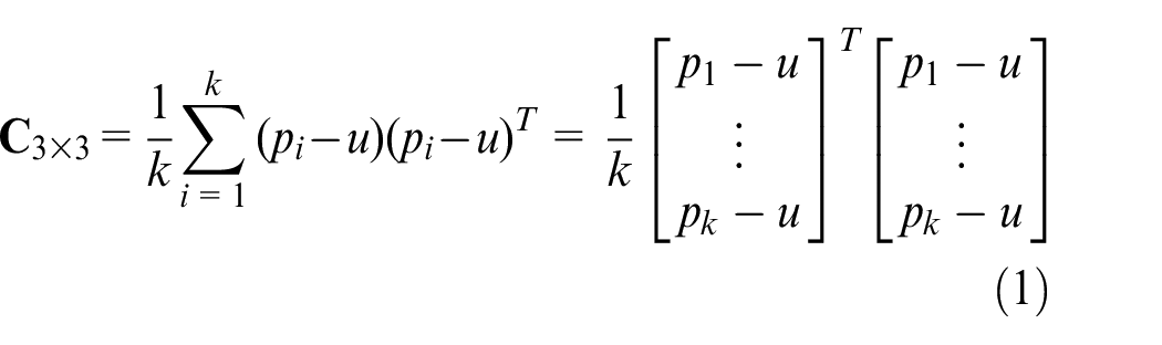
The covariance matrix
The least eigenvalue
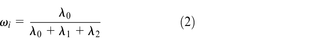
The weight
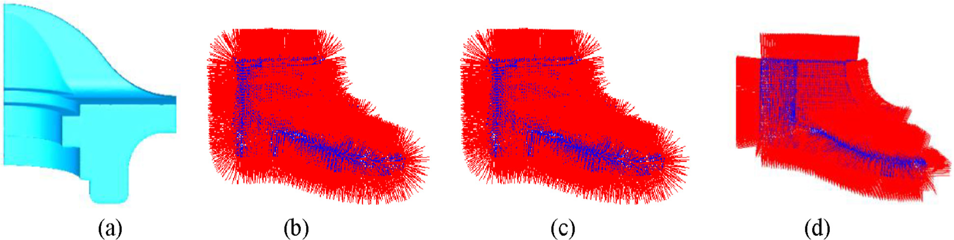
Figure 1(a) is a point cloud model with sharp feature, with the red line representing the intersection of two or more surface patch. Point closes to the intersection areas can be seen as feature points. It can be known that kNN of the feature point located at more than two surface patches. The feature point detection result is shown in Figure 1(b), the red points represent feature points. After the feature point cloud detection, the point cloud can be classified to feature points and non-feature points. The kNN of non-feature points are anisotropic and the kNN of feature points are isotropic. The estimated normal vector based on PCA method is shown in Figure 1(c) with the red line representing normal vector. Since the directions of normal vectors are not consistent, they are adjusted to the same direction for displaying. It can be seen from Figure 1(c), normal vector of feature point in intersection area is not perpendicular to the local planar surfaces because kNN used to fit a local plane are from at least two surface patches. In this case, the estimated normal vectors are inaccuracy, and normal vectors of feature points are regarded as smoothed.
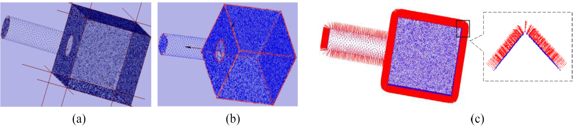
Feature points detection and normal estimating results for point cloud model based on PCA method; (a) point cloud model; (b) feature point cloud estimation result; (c) normalized normal vectors.
The PCA method can be used to estimate normals of points for smooth surface rapidly, that means normals of points are accurate in flat area instead of feature area. To obtain more accurate normal, the normals need to be refined. Lee et al.
29
extend the bilateral filtering to refine the normal of triangular faces of the mesh. Given a triangular face fi with a unit normal
Where
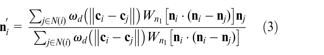
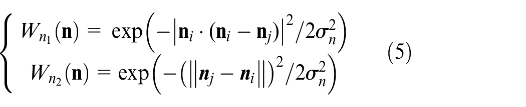
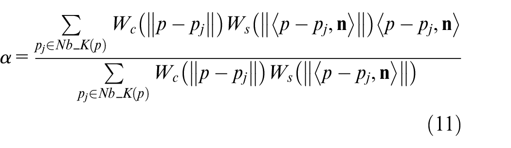
Similarly, in our previous work, 23 we proposed an improved bilateral normal filtering to refine the normal of point cloud as follows:
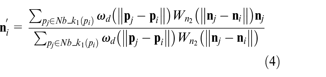
where
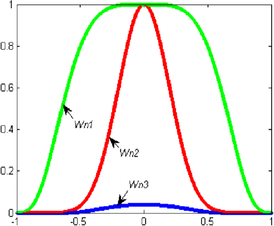
The distribution of three different weights.
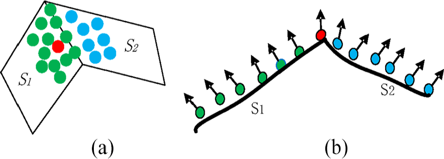
Schematic of point cloud and normal vector; (a) point cloud in two surface patches; (b) normal vector before refining.
Figure 3 is the schematic of point cloud and normal vector before refining in two surface patches, where the red point represents the feature point. The kNN of feature points are located at two surface patches, and the blue points in surface patch S2 can be regard as noise or outlier for point in surface S1 when normal vector refining. Although the kNN of feature point locate at two surface patches at least, most of neighbors of feature points are non-feature points. Normal vectors of non-feature points are similar to each other because some of neighbor points are located at one surface patch. When neighbor points are located at different surface patches, normals of these points are deviated from each other; the surface is sharper; the angle of normal vector between different points is larger.
Even though equation (4) decreases the effect of noise point, it still exists with a certain value. Consequently, more iteration times are required to refine the normal vector. To tackle this problem, we optimize equation (4) as follows:
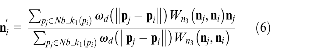
where
where
Essentially, we truncate the normal vectors if the difference between them and
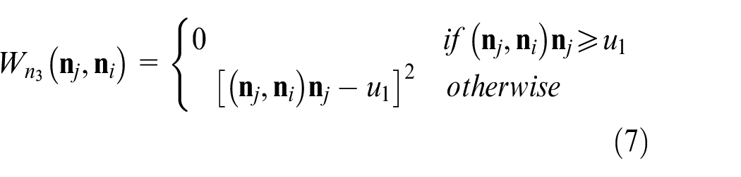
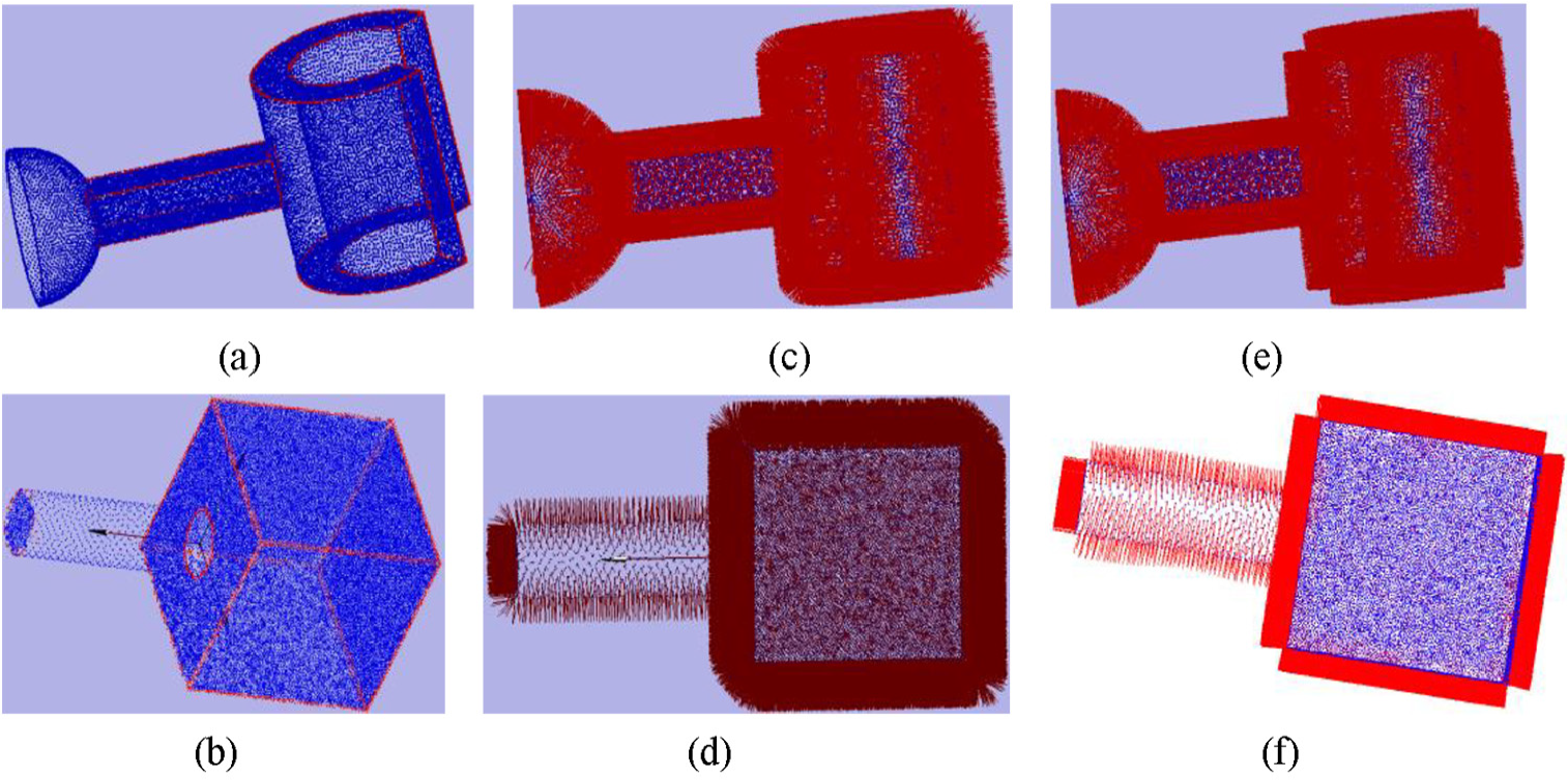
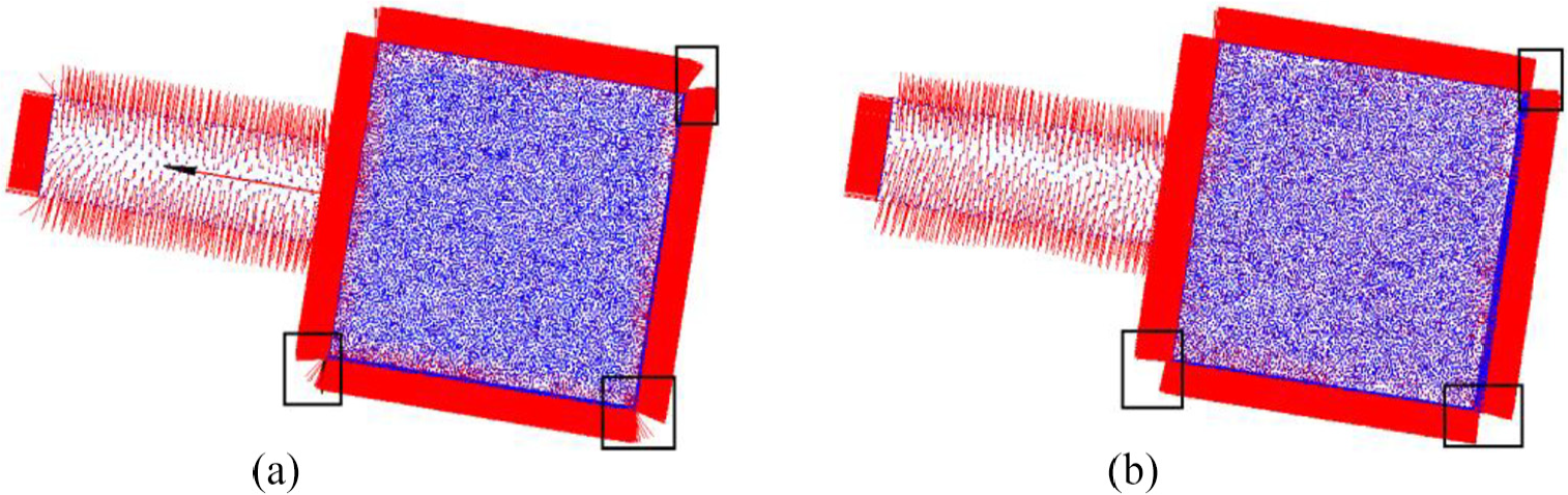
In order to improve the computational efficiency, only normals of feature points are refined. Figure 4 is the normal refine results for two different point cloud model. It can be seen that the refined normal vector is nearly perpendicular to the corresponding local surface. For comparison, the refined normal based on our method and our previous work 23 is shown in Figure 5. Three iterations are performed for both methods when normal refining. The detailed comparison result can be seen the black rectangular area. It can be seen that our method can obtain more precision results for normal refining with the same iteration.
Normal refining result for point cloud; (a), (b) are the point cloud models; (c), (d) are normal estimation results based on PCA method; (e), (f) are normal refining results.
Anisotropic neighborhood seaching
To get the anisotropic neighborhood, the isotropic neighborhood is divided into several sub- neighborhoods by mapping the isotropic kNN into Gaussian image.
Let
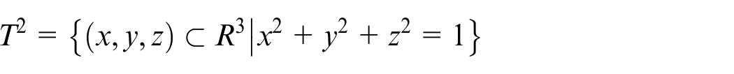
The resulting map
The Gaussian image has very important property: If a connected surface is a plane, the Gaussian image of the point on that surface is a point; Conversely, if the Gaussian image of a connected surface is a point, all the points on that surface are planar points. 20 However, there is always error between estimated normal and ground-truth normal. Therefore, the Gaussian image of point cloud dataset in a planar surface display a cluster where data is in dense distribution. Figure 6(a) shows the sketch map of Gaussian image of planar surface
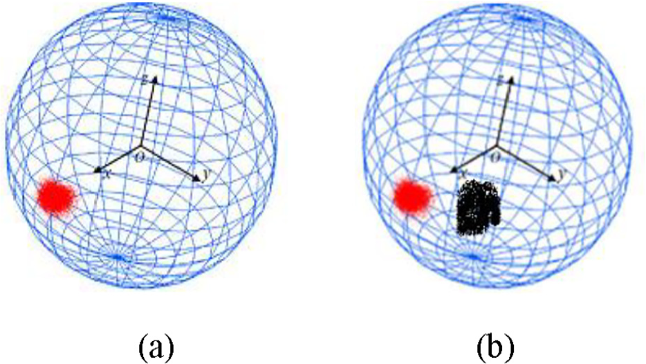
Schmatic plot of Gaussian map; (a) Gaussian map of planar surface; (b) Gaussian map of dihedral surface patch.
If the estimated normal vector is approximated to the ground-truth normal, for a point locating at the surface edge area, its kNN points may be from two surface, that the kNN points in Gaussian map displaying two dense clusters; And for a point locating at the surface corner area, its Gaussian map displays several clusters, and the number of clusters equals to that of surface patches. Figure 6(b) shows the schematic plot of Gaussian image of dihedral surface, where the red and black clusters correspond to points from two different surfaces patches. Therefore, the clustering algorithm is necessary to separate the data into appropriate cluster on Gaussian sphere.
To segment the isotropic neighborhood of feature points pi, a larger neighbors
Mean shift algorithm and hierarchical agglomerative algorithm are non-parameter clustering algorithms to cluster data set without specifying the number of cluster, widely used in data mining and machine vision area. However, it is found that the mean shift algorithm usually classifies one cluster data with too many sub-clusters, some of which may just contain one or two points. The hierarchical agglomerative (”bottom-up”) clustering method 31 was employed to classify data in the work. It begins with each point as a separate cluster, and merges them successively into larger clusters. For the hierarchical agglomerative clustering algorithm, it is an important step to determine the similarity between two clusters.
There are three classic standards, which are single-linkage, complete-linkage and average-linkage measures, to define the distance between two clusters. The average-linkage standard defining the mean distance Dc between elements of each cluster tends to merge two clusters with small difference. It is used to define the distance between two clusters in the work.
The data set
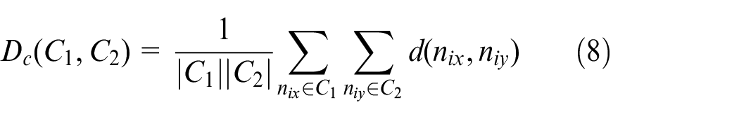
where

where
Results and discussion
Parameter selection
There are five parameters influencing the neighborhood searching result, requiring the user to prepare in the algorithm. They are Thresh, t, k, k2, and
Feature point detection threshold Thresh requires the user to prepare for selecting the feature point where neighbors should be segmented, and normal needs to be modified. The sharpness threshold is related to the “sharpness” of the features of the point cloud. If the surface of point cloud contains very sharp features, it should be a small value; otherwise, it is assigned with a relatively high value. Based on the experimental, the value of Thresh can be 0.001 to 0.1.
t is the iteration time to refining the normal vector. We have the setting in our implementation: t: [1–5].
k is the size of nearest neighborhood, representing the KD tree neighborhood of point data for user to define. After establishing KD tree for point cloud, the kNN of the point cloud are selected by user. When a point is non-feature, the kNN is the final neighbor.
k 2 is the size of nearest neighborhood of feature point, with neighbors mapped into Gaussian image. Usually, the k2-nearest neighbors are isotropic, segmented into several sub-neighbors that are anisotropic. The value of k2 is associated with k. Since the feature point is close to the area of intersection of two or more surface patches, we need to consider the surface complexity to set the value of k2, thus making the neighbor size of feature point close to the neighbor of regular point as much as possible,.
For example, if the feature points are the intersection of two or more surface patches, it can be set as k2 = 2k; if the feature points are the intersection of three or more surface patches, then it can set as k2=3k. It is assumed k2 = 3k, and k = 16 in default in this work.
Parameter
The sharper surface patch leads to the larger angle between normal vectors of points in different surface patch.
Applications of point cloud neighborhood
In order to verify the validity of our algorithm, the anisotropic neighbors of point cloud are applied to point data processing. We compare our proposed method with the state-of-the-art neighborhood searching algorithms, such as KD tree 14 and 3D grid 13 kNN searching method. These algorithms are implemented using Microsoft vision studio 2017 C++, and OpenGL. Since it is hard to visualize neighbors for every point, the neighbors of point are applied for data processing, for example, normal estimation based on local surface fitting, and point data denoising. In the comparison, all the parameters are same except for neighbors.
Normal estimation based on local surface fitting
Normal vector is an important property of a 3D surface. Many effective point cloud processing algorithms depend on the accurate normal as input to produce a precise processing result. The normal estimation can be applied in point cloud denoising, simplification, registration and surface reconstruction. LSF method estimates the normal vector by fitting the least square tangent plane using the local neighborhoods. If neighborhoods of point are anisotropic, the estimated normal is nearly perpendicular to the local tangent plane which means normal are accurate. LSF method is used to estimated normal vector with the KD tree, 3D grid and our anisotropic neighbors as input.
Figures 7 and 8 shows the visualization results of normal vectors based on different neighborhoods as input. Octahedral and fandisk model consists of many continuous surface patches, and feature boundaries can be observed clearly. Normals are normalized and adjusted to the consistent direction for displaying. It can be known that the normal vector of point is nearly perpendicular to the local surface in flat area for 3D grid and KD tree neighbor as input. However, the normal vector of feature point is smoothed, deviated from the local surface because the neighbors of feature point are from at least two surface patches. The estimated normal vectors based on our neighbors are accurate in flat area and feature points because neighbors of feature points are anisotropic, only located at one continuous surface patch.
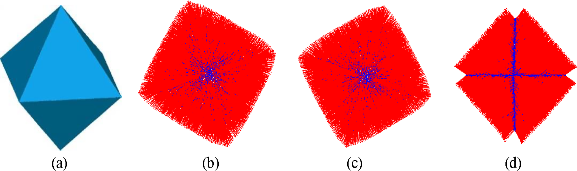
Normal vector estimation results for octahedral model based on different neighbors as input: (a) Triangulated model of octahedral point cloud; (b) KD tree neighbor; (c) 3D grid neighbor; (d) Our neighbor.
Normal vector estimation results for findisk model based on different neighbors as input: (a) Triangulated model of fandisk point cloud; (b) KD tree neighbor; (c) 3D grid neighbor; (d) Our neighbor.
Point cloud denoising
With the development of 3D scanner, it is very convenient to acquire 3D point cloud. However, the collected point cloud data inevitably contains noise due to a variety of internal and external factors interference. Denoising is necessary step to improve the data quality for further data processing. The main problem of point cloud denoising is to remove noise while preserving sharp feature.
Bilateral filtering algorithm
33
can be used to denoise for point cloud and mesh surface while preserving the sharp feature; however, it needs the accurate normal and neighbors as input. Bilateral filtering denosing for point cloud is given as follows: Let

where
Where
To highlight the influence of neighborhood on denoising results, normal of point is estimated by method introduced in the Literature. 26 It can accurately estimate normal vector and robust to noise. Two point cloud which contain sharp feature are employed to test denoising results.
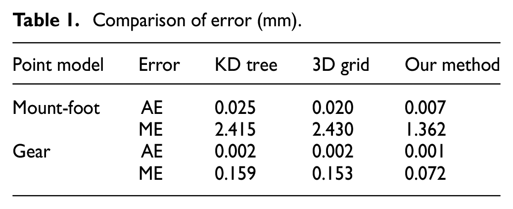
Figures 9 and 10 show the denoising results based on 3D grid, KD tree and our neighbors as input
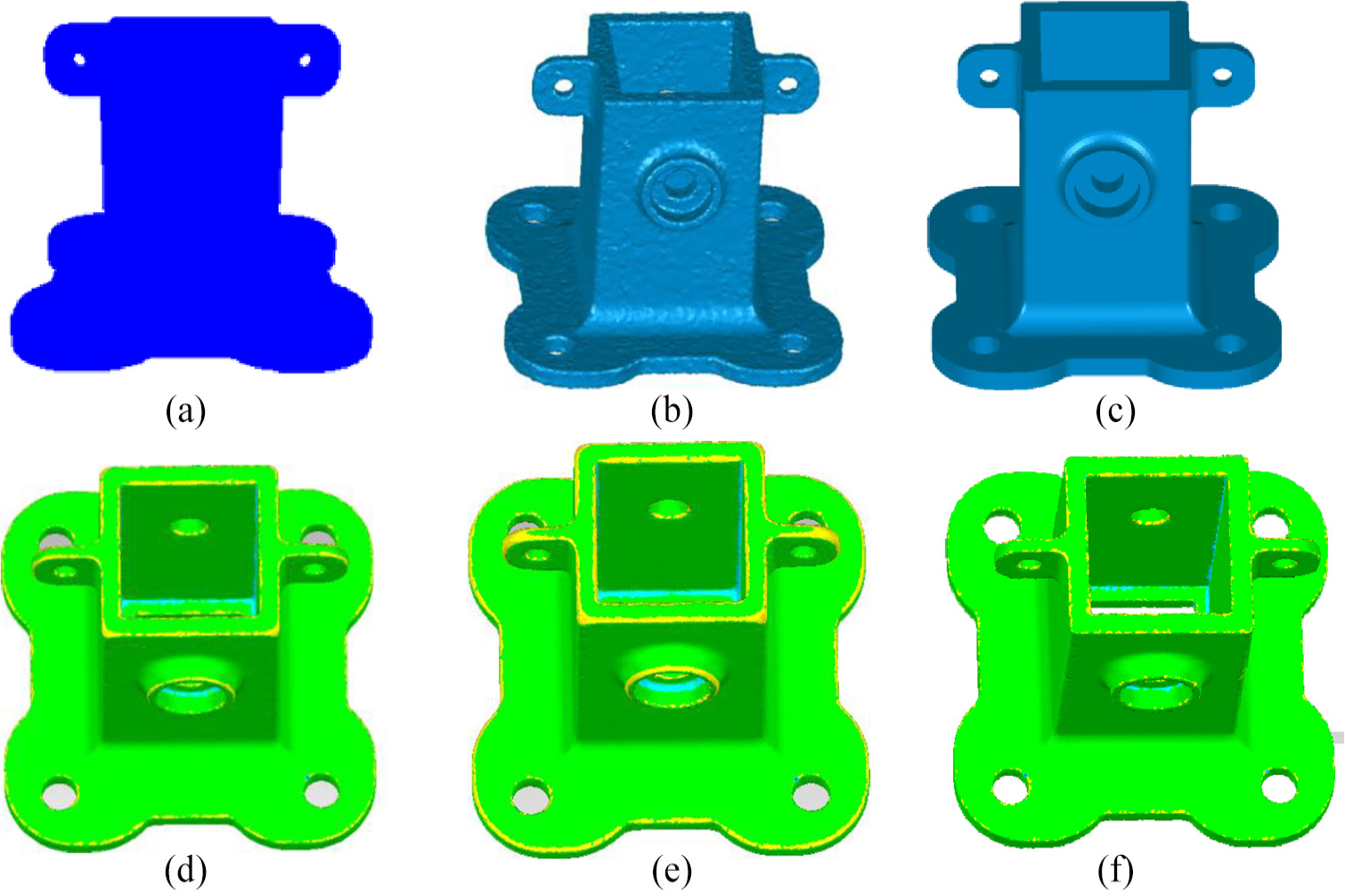
Bilateral filter denoising results for mounting-foot model with KD tree, 3D grid and our neighbors as input; (a) mounting-foot point cloud model with noise; (b) triangulation of Figure 9(a); (c) triangulation of mounting-foot model with noise-free; (d)–(f) Denoising and deviation results based on KD tree, 3D grid and our method, respectively.
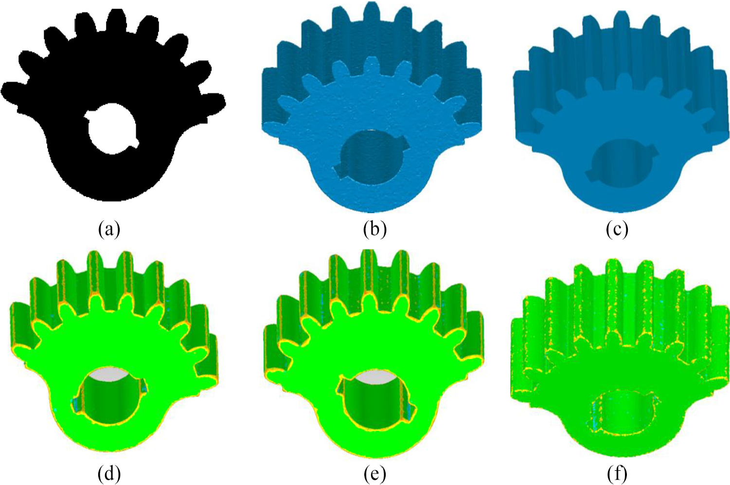
Bilateral filter denoising results for gear model with KD tree, 3D grid and our neighbors as input; (a) gear point cloud model with noise; (b) Triangulation of Figure 10(a); (c) Triangulation of gear model with noise-free; (d)–(f) Denoising and deviation results based on KD tree, 3D grid and our method, respectively.
Comparison of error (mm).
Computational time analysis
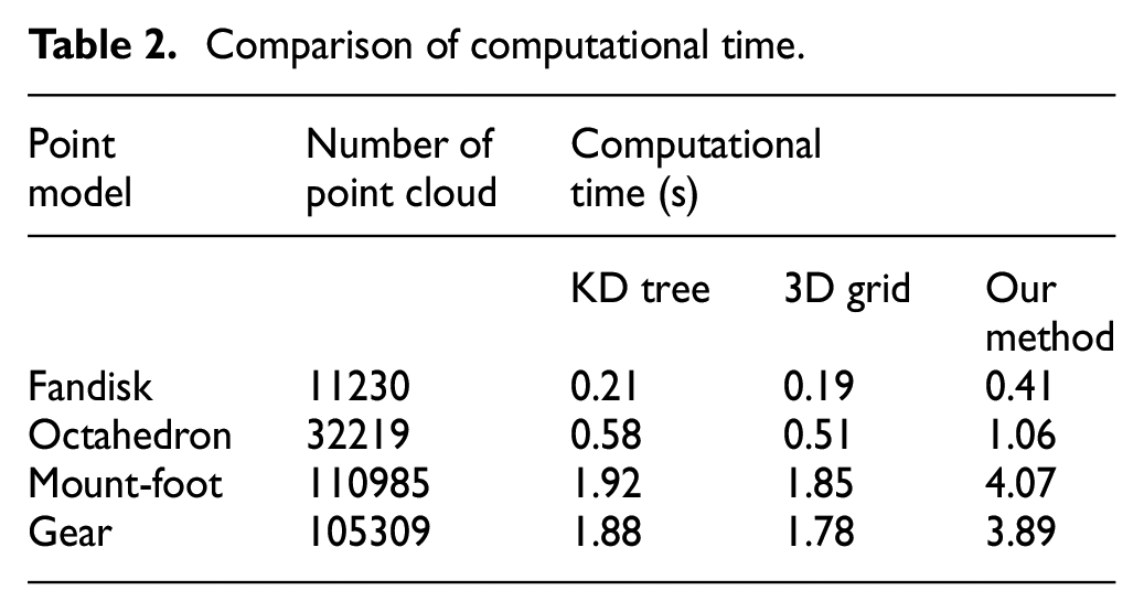
Our proposed method needs to fit a local tangent plane to estimate normal vector and detect feature points, and normal vectors of these points are iteratively refined. After hierarchical clustering in Gaussian sphere, isotropic neighbors are classified into several anisotropic sub-clusters besides constructing KD tree. Therefore, it is more computational than the neighborhood searching method by 3D grid and KD tree. Test computations are implemented on a PC with a 2.5 GHz Intel Core processor and 16 GB RAM. Table 2 shows the results of computational time for different point cloud. Different computers take different amounts of time to execute the algorithm, thus, the computational time in Table 2 just for reference. According to the computational complexity and Table 2, it is obvious that our method is more time-consuming that several times larger than that required by the method of 3D grid and KD tree.
Comparison of computational time.
Conclusion
The neighborhood searching of point data is very import and a basic work for point cloud processing. A large amount of point data processing algorithms need neighbors as input to produce precise processing result, such as normal estimation, denoising, and reconstruction. Since the kNN of feature points is isotropic that may contain points belonging to more than two surface patches, sharp feature of point cloud model are over-smoothed with these neighbors as input for point processing. An anisotropic neighborhood searching method was proposed in the work.
Our method divides a big isotropic kNN of feature points into several anisotropic sub-neighborhoods by mapping the big isotropic kNN neighbors into a Gaussian sphere. The points on Gaussian image formed several sub-clusters corresponding to the anisotropic sub-neighbors. The agglomerative hierarchical clustering algorithm was used to separate the data in Gaussian image into appropriate cluster. The biggest sub-neighborhood corresponding to the biggest sub-cluster was selected as the optimal anisotropic neighbors. Since a large kNN of feature point was segmented into a series of sub-neighbors, the number of neighbors of point is not same everywhere. Neighbors of points are applied to estimate normal and bilateral filtering denoising.
K nearest neighborhood usually is isotropic for point cloud with sharp feature, different from the other k nearest neighborhood search methods, this paper emphasizes on the anisotropic neighborhood searching instead of computational efficiency. Point cloud normal estimation and denoising based on 3D grid, KD tree and our neighbors as input, our method can obtain more precision result for point cloud with sharp feature. The anisotropic neighborhood searching based on our method can be used for point cloud normal estimation, denoising, surface fitting, and reconstruction, et al. It is important to point out that the method in the work is more computational and complex than DR and SP neighborhood searching method. The future work will improve the computational efficiency and reduce complexity for searing anisotropic neighborhood.
Footnotes
Acknowledgements
The authors would like to thank Jiangxi Province Education Department, Jiangxi provincial department of science and technology, National Natural Science Foundation of China and our previous work20 to support this work.
Author contributions
Xiaocui Yuan proposed the idea of this algorithm, and wrote programs to implementation our algorithm and other correlation algorithm. Baoling Liu designed the framework of this paper. Yongli Ma was responsible for data collection and modified paper.
Declaration of Conflicting Interests
The author(s) declared no potential conflicts of interest with respect to the research, authorship, and/or publication of this article.
Funding
The author(s) disclosed receipt of the following financial support for the research, authorship, and/or publication of this article: This work is support by Jiangxi Province Education Department (Grant No. GJJ161122, GJJ161104, GJJ16110), Jiangxi Provincial Department of Science and Technology (Grant No. 20171BAB206037) and National Natural Science Foundation of China (Grant No. 61903176, 62001202).