Sage Journals: Discover world-class research

Abstract

Parametric interpolation for spline plays an increasingly important role in modern manufacturing. It is critical to develop a fast parametric interpolator with high accuracy. To improve the computational efficiency while guaranteeing low and controllable feedrate fluctuation, a novel parametric interpolation method based on prediction and iterative compensation is proposed in this article. First, the feedrate fluctuation and Taylor’s expansion are analyzed that there are two main reasons to reduce the calculation accuracy including the truncation errors caused by neglecting the high-order terms and discrepancy errors between the original curve and the actual tool path. Then, to reduce these errors, a novel parametric interpolation method is proposed with two main stages, namely, prediction and iterative compensation. In the first stage, a quintic polynomial prediction algorithm is designed based on the historical interpolation knowledge to estimate the target length used in the second-order Taylor’s expansion, which can improve the calculation accuracy and the convergence rate of iterative process. In the second stage, an iterative compensation algorithm based on the second-order Taylor’s expansion and feedrate fluctuation is designed to approach the target point. Therefore, the calculation accuracy is controllable and can satisfy the specified value through several iterations. When finishing the interpolation of current period, the historical knowledge is updated to prepare for the following interpolation. Finally, a series of simulations are conducted to evaluate the good performance in accuracy and efficiency of the proposed method.

Keywords

Parametric interpolation feedrate fluctuation length prediction historical interpolation knowledge iterative compensation second-order Taylor’s expansion

Introduction

Parametric interpolation for spline plays an increasingly important role in modern manufacturing including computer numerical control machining and robots.^1,2 Compared with the traditional linear and circular interpolation, parametric interpolation has a lot of advantages in surface quality, execution efficiency, memory consumption, and motion smoothness and is especially suitable for the high-speed and high-accuracy occasions.^3,4 Therefore, it is critical to develop a reasonable parametric interpolator to realize fast and accurate calculation.

There are two main steps to conduct the parametric interpolation. The first and the key step is to determine the parameter $u_{i + 1}$ of target point in the ith interpolation period based on the step size L_i . Then, in the second step, the position $C (u_{i + 1})$ of target point can be calculated by $u_{i + 1}$ . However, it is more difficult to obtain $u_{i + 1}$ precisely because there is no analytical relation between the arc length and the parameter of spline, which causes feedrate fluctuation and affects the motion smoothness. On the other hand, the real-time performance is another key factor to consider when increasing the calculation accuracy. Therefore, both the feedrate fluctuation and computational time should be regarded as the criteria of an efficient algorithm.

The first- and second-order Taylor’s expansion (STE) are the widely used approximate methods with low computational load^5

–9 and can satisfy the accuracy requirement of general situations. However, the high-order terms are neglected to improve the real-time performance, which causes the truncation errors. Hence, the calculation accuracy is limited and not suitable for the higher requirement. To improve the accuracy, the remapping interpolation methods (RIMs) are developed. The main idea of RIM is to establish the inverse length function (ILF) between the arc length and parameter. The polynomial functions with different orders are widely used to construct ILF. Liu et al.¹⁰ and Lei et al.¹¹ used the cubic polynomial function for interpolation. To further improve the calculation accuracy, quintic polynomial function was employed in the study by Erkorkmaz and Altintas¹² and Jeong.¹³ Moreover, Heng and Erkorkmaz,¹⁴ Yang et al.,¹⁵ and Yang and Altintas¹⁶ adopted the seventh- and ninth-order polynomials to avoid wiggle. With the ILF of each curve segment, the computational load is lower. However, a large amount of polynomial functions are constructed, which needs considerably large memory to store the coefficients. Meanwhile, both the Taylor’s expansion and the RIM cannot control the calculation accuracy to reach the specified value.

To cope with these problems, some feedback interpolation methods, which employed the feedrate feedback schemes to compensate for the feedrate fluctuation in an iterative manner, have been developed. Cheng et al.,¹⁷ Cheng and Tsai,¹⁸ and Cheng et al.¹⁹ proposed the real-time predictor–corrector interpolator with two stages, which reduces the feedrate fluctuation significantly. The predictor stage is to estimate the initial parameter. Then, in the corrector stage, the parameter can be approached through iteration until the feedrate fluctuation satisfies the specified value. To reduce the iteration number, Zhao et al.²⁰ developed the chord-tracking algorithm (CTA). Similarly, CTA has two stages. In the first stage, the arc-length compensation scheme is proposed according to the curvature of the curve, and the STE is employed to predict the parameter. In the second stage, the Newton–Raphson algorithm is used for the iterative correction.

To further improve the computational efficiency while guaranteeing controllable accuracy, a novel parametric interpolation method based on prediction and iterative compensation (PIC) is proposed in this article. First, the feedrate fluctuation and Taylor’s expansion are analyzed that there are two main reasons to reduce the calculation accuracy including the truncation errors caused by neglecting the high-order terms and discrepancy errors between the original curve and the actual tool path. Then, to reduce these errors, a novel parametric interpolation method is proposed with two main stages, namely, PIC. In the first stage, the target length used in the STE is estimated by the proposed prediction algorithm where a quintic polynomial prediction model is established based on the historical interpolation knowledge. The modeling and prediction processes have low computational load because the coefficient matrix in parameter identification is constant. After that, in the second stage, an iterative compensation algorithm based on the STE and feedrate fluctuation is designed to approach the target point. Therefore, the convergence rate can be increased by the length prediction. Meanwhile, the calculation accuracy is controllable and can satisfy the specified value through several iterations. When finishing the interpolation of current period, the historical knowledge is updated to prepare for the following interpolation.

The remainder of this article is organized as follows. In the second section, the analysis of the feedrate fluctuation and Taylor’s expansion is illustrated. The third section describes the proposed parametric interpolation method including PIC. Simulation results are analyzed and compared with previous works in the fourth section. The conclusions are given in the fifth section.

Analysis of feedrate fluctuation and Taylor’s expansion

The typical procedures of spline interpolation are given in the study by Xinhua et al.,²¹ which can be described briefly as follows. In the ith interpolation period, the feedrate scheduling module is implemented firstly to obtain the desired step size L_i . Then, the parametric interpolation module is performed to calculate the position of the target interpolation point. Finally, the motion controller conducts the real-time servo control and drives the motion axes to track the target trajectory. Therefore, the actual tool path in each interpolation period is a small line segment. When conducting the parametric interpolation, there is no relation between the arc length and parameter of the spline, which makes it difficult to realize a fast and accurate interpolation. As shown in Figure 1, where A, B, and C are the start, target, and actual points in the ith interpolation period, the feedrate fluctuation ε is inevitable with the approximate calculation, which can be expressed as follows

ε = | \frac{V_{i} - V_{i}^{*}}{V_{i}} | \times 100 %

V_{i}^{*} = \frac{‖ C (u_{i + 1}) - C (u_{i}) ‖}{T_{s}}

where $V_{i} = \frac{L_{i}}{T_{s}}$ is the desired feedrate, $V_{i}^{*}$ is the actual feedrate obtained by the start point $C (u_{i})$ , the calculated target point $C (u_{i + 1})$ , and the interpolation period T_s . The following equation can be established if the feedrate fluctuation is fully eliminated

L_{i} = ‖ C (u_{i + 1}) - C (u_{i}) ‖

Figure 1.

Feedrate fluctuation in parametric interpolation.

Among the various interpolation methods, the Taylor’s expansion is widely used especially in the first- and second-order expansion for their low computational load, which can be expressed by equations (4) and (5),²² respectively

u_{i + 1} = u_{i} + \frac{\overset{⌢}{L_{i}^{T}}}{‖ C^{'} (u_{i}) ‖} + high order terms

u_{i + 1} = u_{i} + \frac{\overset{⌢}{L_{i}^{T}}}{‖ C^{'} (u_{i}) ‖} - \frac{〈 C^{'} (u_{i}), C ″ (u_{i}) 〉 {\overset{⌢}{L_{i}^{T}}}^{2}}{2 {‖ C^{'} (u_{i}) ‖}^{4}} + high order terms

where $\overset{⌢}{L_{i}^{T}}$ is the length corresponding to the sampling step size L_i , $C^{'} (u_{i})$ and $C ″ (u_{i})$ are the first and second derivatives of the parametric curve at u_i , respectively. However, the calculation accuracy of the first- and second-order expansion is lower with serious and uncontrollable feedrate fluctuation. As shown in Figure 2(a), there are at least two main reasons to reduce the calculation accuracy as follows:

Truncation errors: The use of Taylor’s expansion can be seen as reconstructing a curve $\overset{⌢}{A D}$ to approach the original curve $\overset{⌢}{A B}$ , and the approaching accuracy depends on the order of expansion. Considering the computational load, the high-order terms in equations (4) and (5) are neglected. Therefore, the truncation errors between $\overset{⌢}{A D}$ and $\overset{⌢}{A B}$ are generated, especially for the high-order parametric curves.

Discrepancy errors: Corresponding to the arc-length $\overset{⌢}{A C}$ of the target parametric curve, the actual tool path is $\bar{A C}$ which is a line segment. Hence, the discrepancy errors between straight line and curve with nonzero curvature are always existing.

In most literatures, L_i is used directly to replace $\overset{⌢}{L_{i}^{T}}$ in equations (4) and (5), which cannot consider these two kinds of errors. Some researchers did some improvements to predict the arc length $\overset{⌢}{L_{i}}$ of the target curve corresponding to L_i to replace $\overset{⌢}{L_{i}^{T}}$ , which aims to reduce the discrepancy errors. However, the two kinds of errors are still obvious. For example, the length of $\bar{A B}$ and $\overset{⌢}{A B}$ corresponds to L_i and $\overset{⌢}{L_{i}}$ in Figure 2(a). When $\overset{⌢}{L_{i}}$ is predicted and used in equation (4) or (5), the reconstructed curve by Taylor’s expansion is $\overset{⌢}{A D^{'}}$ , where $\overset{⌢}{A D^{'}} = \overset{⌢}{L_{i}}$ . Then, the point $C^{'}$ on the curve which has the same parameter $u_{i + 1}$ with point $D^{'}$ can be obtained and the actual tool path is $\bar{A C^{'}}$ . It can be seen that the difference between $\bar{A C^{'}}$ and $\bar{A B}$ is still large with the two kinds of errors. Hence, even if ${\overset{⌢}{L}}_{i}$ can be calculated precisely, the accuracy might not be able to satisfy the requirement. However, as shown in Figure 2(b), the accuracy can be improved obviously if $\overset{⌢}{L_{i}^{T}}$ corresponding to L_i can be predicted, which will be given in the third section.

Figure 2.

Analysis of the interpolation accuracy by Taylor’s expansion.

Parametric interpolation method based on PIC

In this section, the proposed parametric interpolation method is described. The prediction algorithm is given in “Quintic prediction algorithm according to historical knowledge” section where a quintic prediction model is established according to the historical knowledge. “Iterative compensation algorithm based on the STE and feedrate fluctuation” section illustrates the iterative compensation algorithm. Finally, the proposed PIC algorithms are combined to construct the parametric interpolation method in “Parametric interpolation method” section.

Quintic prediction algorithm according to historical knowledge

As described in the second section, it is effective to improve the interpolation accuracy by predicting the length $\overset{⌢}{L_{i}^{T}}$ for Taylor’s expansion. However, $\overset{⌢}{L_{i}^{T}}$ relates to many factors including the order and curvature of the target curve, the order of the employed Taylor’s expansion, and the desired L_i by feedrate scheduling. It is difficult to build their analytical relations. In addition, the computational load should be considered to guarantee the real-time performance. Therefore, other forms of prediction algorithm should be designed with fast calculation.

As can be seen from Figure 3, for a definite parametric curve interpolated by Taylor’s expansion with definite order, the curvature and feedrate profiles change gently between the adjacent interpolation periods. Therefore, $\overset{⌢}{L_{i}^{T}}$ can be predicted by the previous interpolation experience which is called historical knowledge.

Figure 3.

Historical knowledge of the interpolation process.

The polynomial functions with different degrees are good at modeling the unknown system and performing the prediction. Hence, the quintic polynomial function is employed to build the prediction model and to predict $\overset{⌢}{L_{i}^{T}}$ . When conducting the interpolation of L_i , the data of previous six periods including the desired length $L_{i - n}$ ( $n = 6 - k$ , $k = 0, 1, 2, 3, 4, 5$ ) and the corresponding length in Taylor’s expansion $\overset{⌢}{L_{i - n}^{T}}$ are used to establish the prediction model. In addition, to decrease the effect from the changes of $L_{i - n}$ and to reduce the number of independent variables, the ratio $R_{i - n}$ of $\overset{⌢}{L_{i - n}^{T}}$ to $L_{i - n}$ is used as the output of the prediction model and k is the input. Therefore, the quintic prediction model can be expressed as follows

R_{i - n} = a_{0} + a_{1} k + a_{2} k^{2} + a_{3} k^{3} + a_{4} k^{4} + a_{5} k^{5}

where a ₀∼a ₅ are the unknown parameters and can be identified as follows

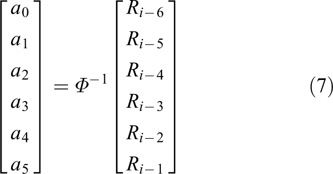
[\begin{matrix} a_{0} \\ a_{1} \\ a_{2} \\ a_{3} \\ a_{4} \\ a_{5} \end{matrix}] = Φ^{- 1} [\begin{matrix} R_{i - 6} \\ R_{i - 5} \\ R_{i - 4} \\ R_{i - 3} \\ R_{i - 2} \\ R_{i - 1} \end{matrix}]

Φ = [\begin{matrix} 1 & 0 & 0 & 0 & 0 & 0 \\ 1 & 1 & 1 & 1 & 1 & 1 \\ 1 & 2 & 2^{2} & 2^{3} & 2^{4} & 2^{5} \\ 1 & 3 & 3^{2} & 3^{3} & 3^{4} & 3^{5} \\ 1 & 4 & 4^{2} & 4^{3} & 4^{4} & 4^{5} \\ 1 & 5 & 5^{2} & 5^{3} & 5^{4} & 5^{5} \end{matrix}]

When predicting $\overset{⌢}{L_{i}^{T}}$ , it only needs to take $k = 6$ and bring it to equation (6). Then, $\overset{⌢}{L_{i}^{T}}$ can be calculated as follows

\overset{⌢}{L_{i}^{T}} = {\hat{R}}_{i} L_{i}

where ${\hat{R}}_{i}$ is the predicted ratio of ith period. Hence, the parameter of target point can be calculated with the STE and $\overset{⌢}{L_{i}^{T}}$ . In order to guarantee the accuracy, the quintic prediction model is used for one-step prediction. Therefore, when the interpolation of ith period is finished, the length $\overset{⌢}{L_{i}^{T}}$ and R_i should be calculated based on equation (5) and used to update the historical knowledge for the prediction of next period.

It should be noted that although equation (6) is a quintic model, the coefficient matrix Φ is constant and its inverse matrix can be obtained in advance. Hence, the parameter identification process given in equation (7) has low computational load. In addition, for the situations that there is no enough historical knowledge such as the beginning part of interpolation process, lower polynomial prediction models can be established similar to equation (6). In particular, the prediction ratio is set to 1 in the first calculation.

Iterative compensation algorithm based on the STE and feedrate fluctuation

The calculation accuracy can be improved by the prediction algorithm given in “Quintic prediction algorithm according to historical knowledge” section. However, the feedrate fluctuation is still uncontrollable and cannot be guaranteed to reach the specified value. Therefore, an iterative compensation algorithm is proposed to cooperate with the prediction algorithm and further reduce the feedrate fluctuation.

Since the computational load of the STE is little larger than the first-order, the second-order method is employed with the feedrate fluctuation to construct the iterative compensation algorithm. Figure 4 illustrates the iterative calculation process in one interpolation period, where E is the start point,F is the desired target point, and F_j is the actual point obtained by the jth iteration. Based on Figure 4, the procedures of the proposed iterative compensation method are described as follows and its flowchart is shown in Figure 5.

Figure 4.

The iterative compensation algorithm.

Figure 5.

The flowchart of the proposed iterative compensation algorithm.

(1) Step 1: initialing iterative parameters

After the feedrate scheduling, the iterative parameters need to be initialed firstly to $j = 1$ , $L_{j} = L_{i}$ , where j is the number of iteration, L_i is the desired sampling step size of the ith period, and L_j is the desired step size in jth iteration.

(2) Step 2: calculating the target point by the STE and L_j .

The parameter u_j of target point can be calculated based on L_j and the STE given in equation (5). Then, F_j can be obtained according to u_j . Hence, the actual length $\bar{E F_{j}^{}}$ can be calculated.

(3) Step 3: calculating the feedrate fluctuation

Based on L_j , $\bar{E F_{j}^{}}$ , and the interpolation period T_s , the feedrate fluctuation ε_j can be calculated by equations (1) and (2). Then, the following judgments should be performed:

If $ε_{j} \leq ε_{d}$ , where ε_d is the specified value, it means that the interpolation calculation of current period is finished. Then, $i = i + 1$ and go to step 1 for the next period.

If $ε_{j} > ε_{d}$ , it means the accuracy should be further improved by iteration. Then, go to step 4.

(4) Step 4: updating j and recalculating the step size L_j based on ε_j

j should be updated by $j = j + 1$ . As can be seen from Figure 4, the step size L_j in next iteration should be equal to $\bar{F_{j - 1}^{} F}$ . However, it is difficult to obtain $\bar{F_{j - 1}^{} F}$ , because F is unknown. Since L_i is small and the curvature of the target curve changes gently in one interpolation period, $∠ F E F_{j - 1}$ is small and $\bar{F_{j - 1}^{} F}$ can be approximated as follows

L_{j} = \bar{F_{j - 1}^{} F} \approx L_{i} ε_{i}

Then, back to step 2.

Through several iterations, the feedrate fluctuation can be reduced to reach the specified value.

Parametric interpolation method

By combining the PIC algorithms, the whole parametric interpolation method can be described as follows and its flowchart is shown in Figure 6. In one interpolation period, there are two main modules.

Figure 6.

The flowchart of the parametric interpolation with prediction and iterative compensation.

Prediction module: Before the interpolation calculation, the quintic polynomial prediction model is established according to the historical knowledge. Then, the ratio ${\hat{R}}_{i}$ for current interpolation period can be predicted and $\overset{⌢}{L_{j}^{T}}$ can be obtained by ${\hat{R}}_{i}$ and L_j .

Iterative compensation module: Based on $\overset{⌢}{L_{j}^{T}}$ , the target point and the corresponding feedrate fluctuation can be calculated by the STE. If the feedrate fluctuation is acceptable, the interpolation of current period is finished. Else, the iterative compensation should be continued. In the following iteration, the compensated L_j can be obtained by equation (10). Because the recalculated L_j is much smaller than L_i , the predicted ratio ${\hat{R}}_{i}$ is no longer used and $\overset{⌢}{L_{j}^{T}} = L_{j}$ for $j > 1$ . After several iterations, the target interpolation point can be obtained with the acceptable feedrate fluctuation.

Simulation validation

In this section, analytical simulations of two nonuniform rational B-spline (NURBS) curves are conducted to evaluate the good performance of the proposed interpolation method with PIC. Analysis and comparisons are also performed with three representative methods including the STE, CTA, and RIM.

Test cases and simulation environment

NURBS is one of the most widely used parametric curve as it offers a common mathematical form for the precise presentation of standard analytical shapes.²³ Therefore, two NURBS curves which are the butterfly-shaped curve and ∞-shaped curve, which are shown in Figure 7 with their curvature curves, are selected as the cases studies. The degree, control points, knot vector, and weight vector of the test curves are given in the study by Ni et al.²⁴ The feedrate scheduling method given in the study by Ni et al.²⁵ is used in this article with the interpolation parameters illustrated in Table 1.

Figure 7.

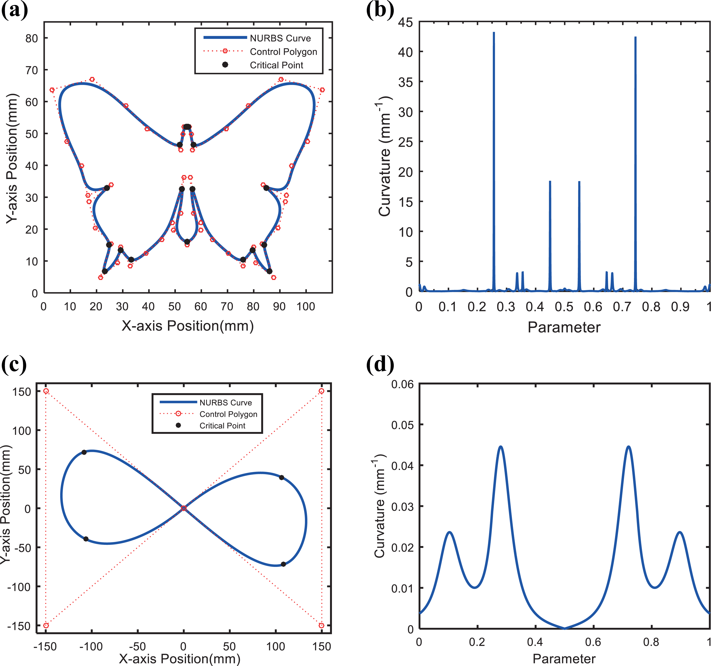
Test curves and their curvature curves. (a) Butterfly-shaped curve, (b) curvature of butterfly-shaped curve, (c) ∞-shaped curve, and (d) curvature of ∞-shaped curve.

The simulations are conducted on a personal computer with Intel(R) Core(TM) i5-4460 3.20-GHz CPU, 4.00-GB SDRAM, and Windows 7 operating system. And all the algorithms for the simulations are developed and implemented on Microsoft visual studio 2008 by C++ language.

Simulation results and comparisons

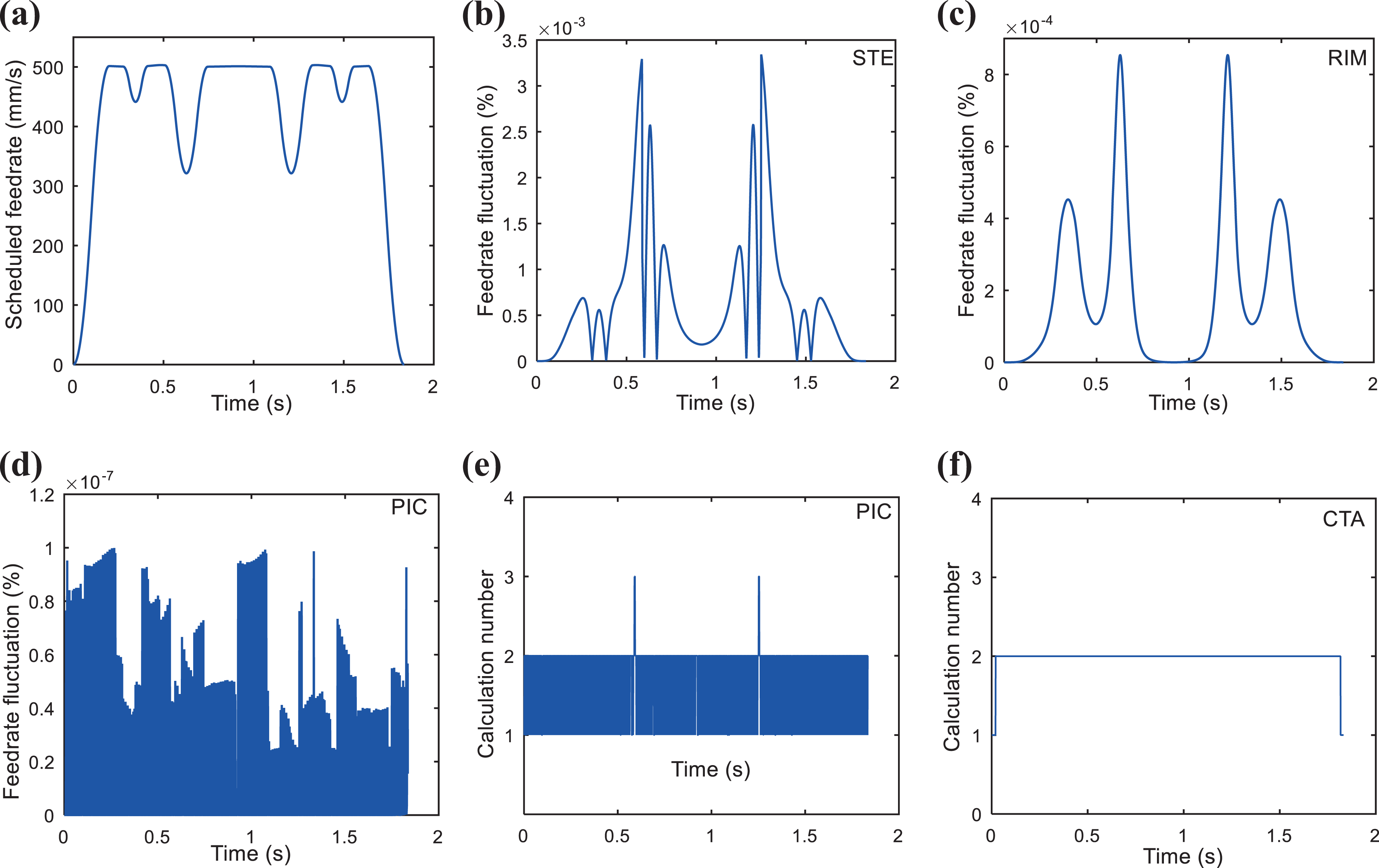
The simulation results of the two NURBS curves are shown in Figures 8(a) to (f) and 9(a) to (f), respectively. As can be seen from Figures 8(b) and (c) and 9(b) and (c), the RIM method has lower feedrate fluctuation than the STE. Meanwhile, the accuracy of these two methods for the ∞-shaped curve is higher than the butterfly-shaped curve owing to the small curvature. However, both of them can only satisfy the low requirement of feedrate fluctuation. In addition, the accuracy cannot be controlled to reach the specified value. Therefore, these methods are only suitable for the parametric curves with small curvatures and low accuracy requirement.

Figure 8.

Simulation results of the butterfly-shaped curve. (a) Scheduled feedrate, (b) feedrate fluctuation by STE, (c) feedrate fluctuation by RIM, (d) feedrate fluctuation by the proposed PIC method, (e) calculation number in one interpolation period by the PIC method, and (f) calculation number in one interpolation period by CTA. STE: second-order Taylor’s expansion; RIM: remapping interpolation method; PIC: prediction and iterative compensation; CTA: chord-tracking algorithm.

Figure 9.

Simulation results of the ∞-shaped curve. (a) Scheduled feedrate, (b) feedrate fluctuation by STE, (c) feedrate fluctuation by RIM, (d) feedrate fluctuation by the proposed PIC method, (e) calculation number in one interpolation period by the PIC method, and (f) calculation number in one interpolation period by CTA. STE: second-order Taylor’s expansion; RIM: remapping interpolation method; PIC: prediction and iterative compensation; CTA: chord-tracking algorithm.

There is no doubt that both the PIC and CTA methods can satisfy the requirements of feedrate fluctuation given in Table 1 through iterative calculation. The calculation numbers in one interpolation period are shown in Figures 8(e) and (f) and 9(e) and (f) and summarized in Table 2. As can be seen, for both the butterfly-shaped and ∞-shaped curves, the calculation numbers by the PIC method are mainly concentrated for one or two times. For the CTA method, the calculation numbers are concentrated for two or three times of butterfly-shaped curve and two times of ∞-shaped curve. The average computational time during each interpolation period is also tested and illustrated in Table 2. As can be seen, the computational time of the butterfly-shaped curve obtained by the PIC method is 3.007 µs which is 24.66% smaller than 3.991 µs obtained by the CTA method. Similarly, for the ∞-shaped curve, PIC method with 2.383 µs is 30.20% faster than the CTA method with 3.414 µs. Therefore, the proposed PIC method has higher computational efficiency and can satisfy the real-time requirement of typical applications.

Table 1.

Interpolation parameters.

Parameters	Butterfly-shaped curve	∞-shaped curve
Interpolation period, T_s (ms)	1	1
Arc length tolerance, δ _arc (mm)	10⁻⁶	10⁻⁶
Maximum chord error, δ _cho (μm)	1	1
Numerical method tolerance, δ _num	10⁻⁴	10⁻⁴
Command federate, F (mm/s)	100	500
Maximum centripetal acceleration, $a_{max c}$ (mm/s²)	3000	4600
Maximum tangential acceleration, $a_{max t}$ (mm/s²)	3000	4600
Maximum jerk, J _max (mm/s³)	55,000	51,000
Feedrate fluctuation tolerance, ε_d	10⁻⁷	10⁻⁷

Table 2.

Static comparisons of the computational efficiency.

Test case	Methods	Ratio of the calculation number				Average computational time (µs)
Test case	Methods	One time (%)	Two times (%)	Three to five times (%)	Greater than five times	Average computational time (µs)
Butterfly-shaped curve	PIC	13.39	78.40	8.21	0	3.007
Butterfly-shaped curve	CTA	0.04	86.71	13.25	0	3.991
∞-shaped curve	PIC	17.27	82.29	0.44	0	2.383
∞-shaped curve	CTA	1.97	98.03	0	0	3.414

PIC: prediction and iterative compensation; CTA: chord-tracking algorithm.

Conclusion

In this article, a novel parametric interpolation method based on PIC is proposed to reduce the computational load while guaranteeing low and controllable feedrate fluctuation. The main conclusions of the study are as follows:

The Taylor’s expansion and feedrate fluctuation are analyzed where there are two main errors, namely, truncation and discrepancy. It is concluded that the calculation accuracy can be improved obviously by predicting the length used in Taylor’s expansion.

To predict the length used in Taylor’s expansion, a quintic polynomial prediction algorithm is proposed based on the historical interpolation knowledge, which can improve the calculation accuracy and increase the convergence rate of iterative process.

An iterative compensation algorithm is designed based on feedrate fluctuation and STE to approaching the target point.

By combining the PIC algorithms, the parametric interpolation method is proposed. Therefore, the convergence rate is increased by the length prediction while the accuracy is guaranteed by iteration.

A series of simulations are performed with previous works to validate the good performance of the proposed method in accuracy and efficiency.

Footnotes

Declaration of conflicting interests

The author(s) declared no potential conflicts of interest with respect to the research, authorship, and/or publication of this article.

Funding

The author(s) disclosed receipt of the following financial support for the research, authorship, and/or publication of this article: The work was supported by the National Key Research and Development Program of China (Grant No. 2017YFB13041102) and the National Natural Science Foundation of China (Grant No. 51875323).

ORCID iD

Chengrui Zhang

Chao Chen

References

Yang

Yuen

. An analytical local corner smoothing algorithm for five-axis CNC machining. Int J Mach Tools Manuf 2017; 123: 22–35.

Huang

Zhu

. A complete S-shape feed rate scheduling approach for NURBS interpolator. J Comput Des Eng 2015; 2(4): 206–217.

Liu

Yuan

. High accurate interpolation of NURBS tool path for CNC machine tools. Chin J Mech Eng 2016; 29(5): 911–920.

Liu

Sun

. A polynomial equation-based interpolation method of NURBS tool path with minimal feed fluctuation for high-quality machining. Int J Adv Manuf Technol 2017; 90(9–12): 2751–2759.

Xie

. Adaptive parametric interpolation scheme with limited acceleration and jerk values for NC machining. Int J Adv Manuf Technol 2008; 36(3–4): 343–354.

Liu

Guo

. An accurate adaptive NURBS curve interpolator with real-time flexible acceleration/deceleration control. Robot Comput-Integr Manuf 2010; 26(4): 273–281.

Dong

Chen

. An accurate NURBS curve interpolation algorithm with short spline interpolation capacity. Int J Adv Manuf Technol 2012; 63(9–12): 1257–1270.

Lee

Lin

Pan

. The feedrate scheduling of NURBS interpolator for CNC machine tools. Comput-Aided Des 2011; 43(6): 612–628.

Sun

Zhao

Bao

. A novel adaptive-feedrate interpolation method for NURBS tool path with drive constraints. Int J Mach Tools Manuf 2014; 77: 74–81.

10.

Liu

Huang

Yin

. Development and implementation of a NURBS interpolator with smooth feedrate scheduling for CNC machine tools. Int J Mach Tools Manuf 2014; 87: 1–15.

11.

Lei

Sung

Lin

. Fast real-time NURBS path interpolation for CNC machine tools. Int J Mach Tools Manuf 2007; 47(10): 1530–1541.

12.

Erkorkmaz

Altintas

. High speed CNC system design. Part I: jerk limited trajectory generation and quintic spline interpolation. Int J Mach Tools Manuf 2001; 41(9): 1323–1345.

13.

Jeong

Choi

Park

. Parametric interpolation using sampled data. Comput-Aided Des 2006; 38: 39–47.

14.

Heng

Erkorkmaz

. Design of a NURBS interpolator with minimal feed fluctuation and continuous feed modulation capability. Int J Mach Tools Manuf 2010; 50(3): 281–293.

15.

Yang

Liu

. Kinematics model and trajectory interpolation algorithm for CNC turning of non-circular profiles. Precis Eng 2018; 54: 212–221.

16.

Yang

Altintas

. Generalized kinematics of five-axis serial machines with non-singular tool path generation. Int J Mach Tools Manuf 2013; 75: 119–132.

17.

Cheng

Tsai

Kuo

. Real-time NURBS command generators for CNC servo controllers. Int J Mach Tools Manuf 2002; 42(7): 801–813.

18.

Cheng

Tsai

. Real-time variable feed rate NURBS curve interpolator for CNC machining. Int J Adv Manuf Technol 2004; 23(11): 865–873.

19.

Cheng

Tsai

Maciejowski

. Feedrate control for non-uniform rational B-spline motion command generation. Proc Inst Mech Eng Part B: J Eng Manuf 2006; 220: 1855–1861.

20.

Zhao

Zhu

Ding

. A parametric interpolator with minimal feed fluctuation for CNC machine tools using arc-length compensation and feedback correction. Int J Mach Tools Manuf 2013; 75: 1–8.

21.

Xinhua

Junquan

Lei

. A novel approach for NURBS interpolation through the integration of ACC-jerk-continuous-based control method and look-ahead algorithm. Int J Adv Manuf Technol 2017; 88(1–4): 961–969.

22.

Koren

Shpitalni

. CNC interpolators: Algorithms analysis. American Society of Mechanical Engineers, Production Engineering Division, 1993, pp. 83–92.

23.

Piegl

Tiller

. The NURBS Book. Berlin: Springer, 1997, pp. 133–158.

24.

Yuan

. Feedrate scheduling of NURBS interpolation based on a novel jerk-continuous ACC/DEC algorithm. IEEE Access 2018; 6: 66403–66417.

25.

Zhang

. An optimized feedrate scheduling method for CNC machining with round-off error compensation. Int J Adv Manuf Technol 2018; 97(5–8): 2369–2381.

A parametric interpolation method based on prediction and iterative compensation

Abstract

Keywords

Introduction

Analysis of feedrate fluctuation and Taylor’s expansion

Parametric interpolation method based on PIC

Quintic prediction algorithm according to historical knowledge

Iterative compensation algorithm based on the STE and feedrate fluctuation

Parametric interpolation method

Simulation validation

Test cases and simulation environment

Simulation results and comparisons

Conclusion

Footnotes

Declaration of conflicting interests

Funding

ORCID iD

References