
Abstract
Due to the reliable feedrate fluctuation and computation load of the existing parametric curve interpolation, a fast interpolation method by cubic B-spline for parametric curve is presented which results in a minimum feedrate fluctuation and light computation load. As there are many geometry implementation tools and many good properties in the B-spline compared with the polynomial, the relation between the arc length s and curve parameter u can be fitted by the cubic B-spline accurately. Because the feedrate fluctuation of the generally used Taylor approximation method is sensitive to the curvature of the toolpath, its accuracy cannot be controlled. For a given feedrate fluctuation of 0.05%, the proposed interpolation method can guarantee the error requirements by increasing the number of the control points. After the de Boor method is applied in real time, the computation load of the cubic B-spline interpolation is decreased compared with the Taylor approximation method and higher order polynomial-fitting method. In order to save the memory consumption for storing the parameters of the fitted cubic B-spline, an iterative optimization process is applied to obtain the knot vector elements and optimize the control points. Simulations and experiments show that the interpolation method can attain high accuracy and computation efficiency. According to the simulations, for most of the complex curves, the feedrate fluctuation of the proposed interpolation method is decreased by about 50% when the feedrate is scheduled and the computation load of the proposed method is decreased by about 70% compared with the second-order interpolation method.
Introduction
Machining aerospace parts, biomedical components, and optical lens comprising complex sculptured surfaces at high speed motivates many researches in the parametric curve interpolation. In contrast to linear interpolation, the parametric curve interpolation is widely applied for machining the complex sculptured surfaces due to the high precision and efficiency.1,2 In parametric interpolation process, the arc length or the feedrate is obtained from the feedrate scheduling process,3,4 and the interpolator calculates the curve parameter according to the arc length or feedrate in real time. But for most of the parametric curves, there is an analytic function that represented the relationship of the arc length s and curve parameter u. As a result, how to accurately calculate the curve parameter in each interpolation period is a tough and meaningful thing.
Various parametric interpolation methods have been proposed to improve the computational accuracy and to reduce the real-time computation load. These methods can generally be classified into two types: online estimate (OE) method and off-line fitting (OF) method. However, none of these methods can consider all the machining requirements which include the arc-length accuracy, computation robustness, the computation load, and memory consumption. For the OE interpolation method, the memory consumption is less than the OF method and it is also easy to operation. But the robustness, accuracy, and real-time computation complexity of the off-line fitting method (OF) are much better than OE interpolation method.
The OE methods are almost depend on the Taylor’s expansion of the relationship between the arc length s and curve parameter u. Huang and Yang 5 proposed the first Taylor expansion method to compute the approximate curve parameter in the next interpolation period. Due to the truncation error, larger feedrate fluctuation is inevitable. Later, Lin 6 and Zhao et al. 7 proposed a second-order approximation; the feedrate fluctuation is reduced compared with the first-order method, but the robustness of this method is limited for some extreme cases. 8 In recent years, some new methods transformed from the Taylor method are issued in order to improve the robustness and accuracy of the Taylor method. Zhao et al. 9 apply a parametric interpolator tool that uses arc-length compensation instead of the chord length to improve the accuracy. Chen et al. 10 designed an augmented Taylor’s expansion method. The new curve parameter is calculated by Henu’s method and a linear parametric interpolation is carried out to cope with the extreme cases. Liu et al. 11 utilized the Taylor expansion on the numerator and denominator in the non-uniform rational basis spline (NURBS) curves to calculate the new curve parameter. Except the above variants of the Taylor expansion method, the Taylor estimate methods that the derivative is replaced by the difference and the accuracy is improved by prediction-correction iteration are also widely applied.12–16 In order to improve the interpolation accuracy, the computation complexity of the OE interpolation method is increased. But there are still many extreme cases, the feedrate fluctuation error requirement cannot be satisfied for the truncation error and accumulated error. Many OE interpolation methods still require extra off-line calculation to increase the interpolator’s robustness and accuracy.
At the same time, OF methods are also adopted in many cases for its less real-time computational load, higher accuracy, and robustness. The correspondence between the arc length s and the parameter u at some points is calculated by a numerical integration method. Then, the relationship between the arc length s and the parameter u is fitted by analytic equations. Piecewise polynomials as fitted analytic equations are widely used in the OF method interpolation. Erkorkmaz and colleagues17–19 adopt quantic and seventh order polynomial to capture the relationship between the spline parameter and the arc displacement. Its accuracy is enhanced by increasing the number of the polynomials and optimizing the polynomials’ coefficient. Later, Lei and colleagues8,20 proposed an inverse length function (ILF) method using cubic/quantic Hermite spline to fit the relationship. There are still many other literatures21,22 that adopt polynomials by choosing different polynomials order or fitting method. In addition to piecewise polynomials, many other forms of analytic equation are also used to represent the relation. Wu et al. 23 established the analytic expansion between the arc length s and parameter u using the bi-arc guide curve.
As the precise and high-speed manufacture requirement increases, the OF method is widely applied for its high accuracy and robustness. But due to the Runge phenomenon of the higher order polynomial interpolation and the accuracy cannot be guaranteed in the mid-points of the piecewise polynomial, the feedrate fluctuation is difficult to be satisfied using the polynomial fitting methods. For the locality and flexibility of the B-spline,
24
a OF interpolation method is proposed using the cubic B-spline, which is called off-line B-spline (OFB) fitting method. The whole OFB fitting process is shown in Figure 1. As shown in Figure 1, the correspondence between the arc length s and the curve parameter u is computed off-line by a numerical integration method. Then, the s-u relationship is fitted by piecewise cubic B-spline. Because the second-order derivative of the cubic B-spline is continuous in a cubic B-spline, the sampled data points are separated according to the
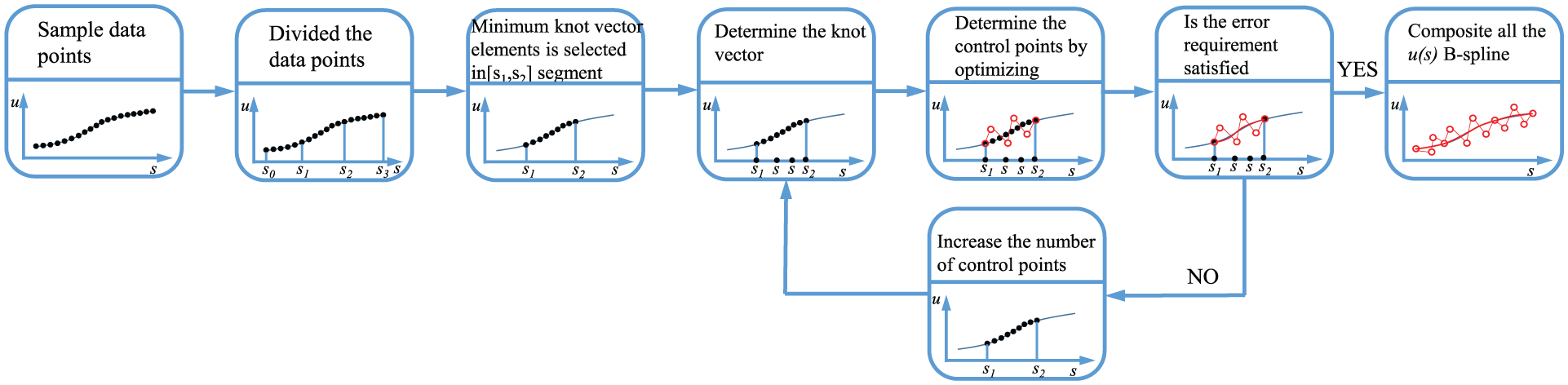
The OFB fitting process.
The B-spline curve and its derivatives
In this article, the relationship between the arc length s and curve parameter u is fitted by cubic B-spline. The definition of a cubic B-spline is given by
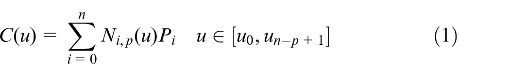
where Pi are the control points and Ni,p(u) are pth degree B-spline basis functions.
The rth derivative of a B-spline can be obtained by de Boor method
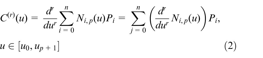
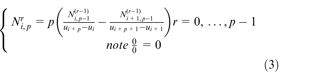
From equation (2), the rth derivative of a pth B-spline is a (p − r)th B-spline. In this article, the cubic B-spline is adopted to fit the relationship between the arc length s and curve parameter u. The third-degree basis function and its nonzero derivatives are shown in Figure 2. As shown in Figure 2, the second derivative of the third basis function is highest order continuous derivative. The third derivative of the third basis function is discontinuous, and it is constant in each knot span. In the following B-spline process, the origin data points are divided according to continuity of the second derivative of the third-degree basis function and the knot vector is distributed by the third derivative of the third-degree basis function.
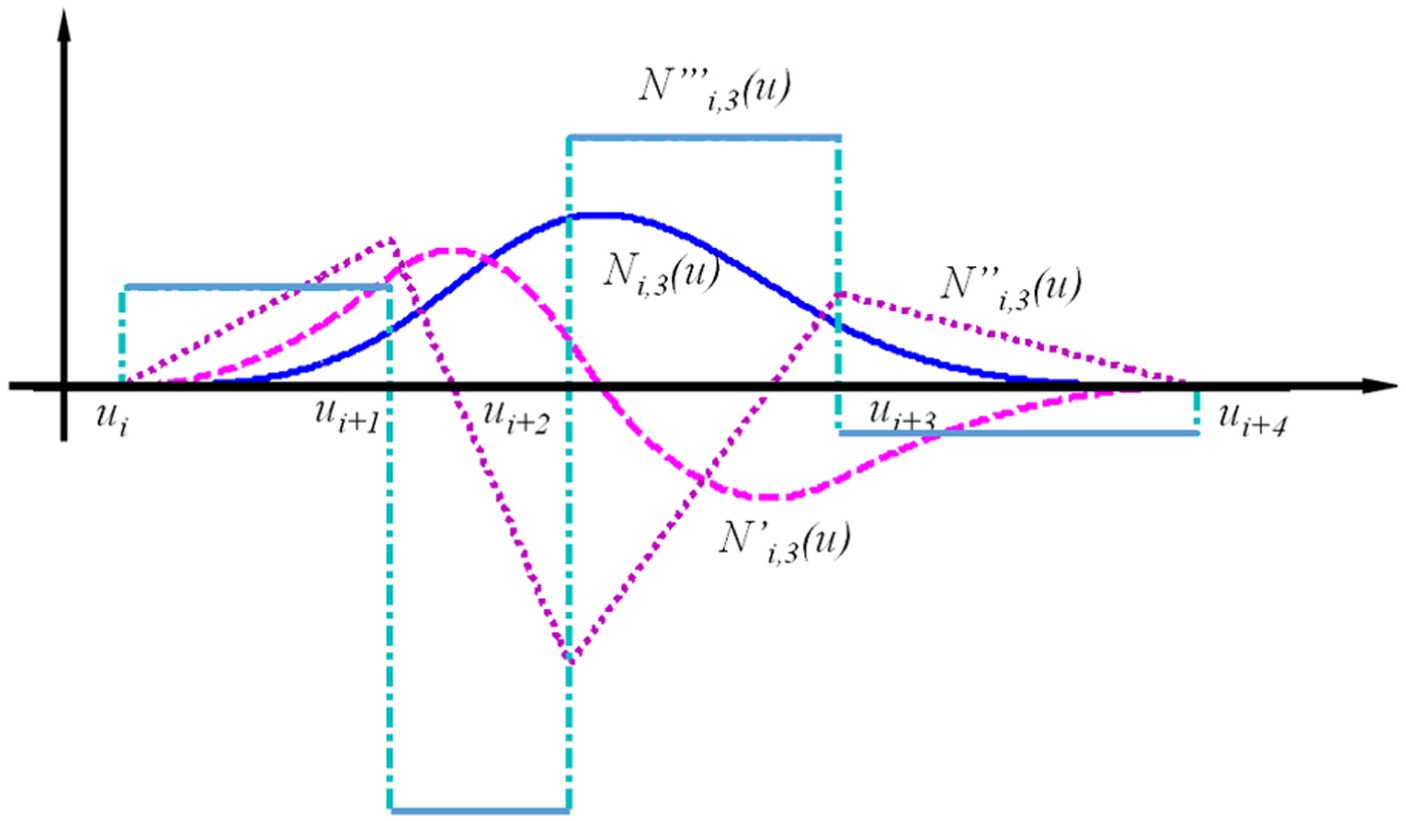
Ni,3 and all its nonzero derivatives.
OF interpolation method by cubic B-spline
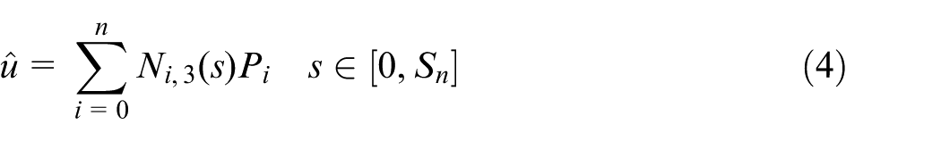
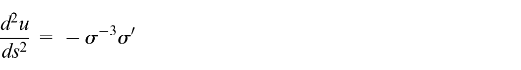
In order to obtain an accurate and robust parameter computation and to lighten the real-time computation burden, an OF interpolation method by cubic B-spline (OFB) is proposed. The relationship between the arc length s and the parameter u is fitted by cubic B-spline
where
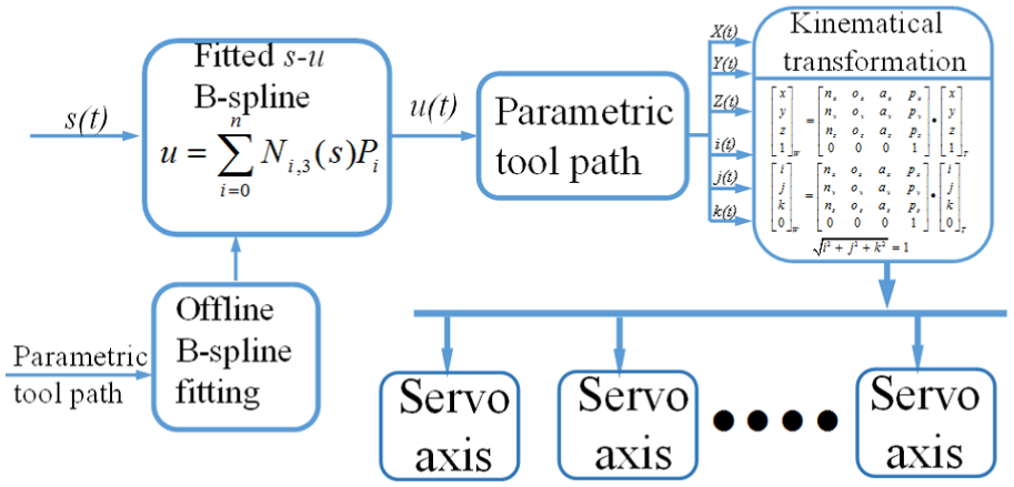
The whole interpolation process.
The arc length calculation of the trajectory
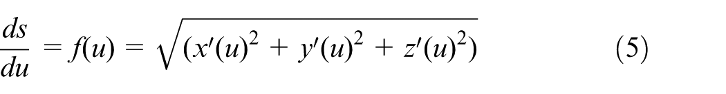
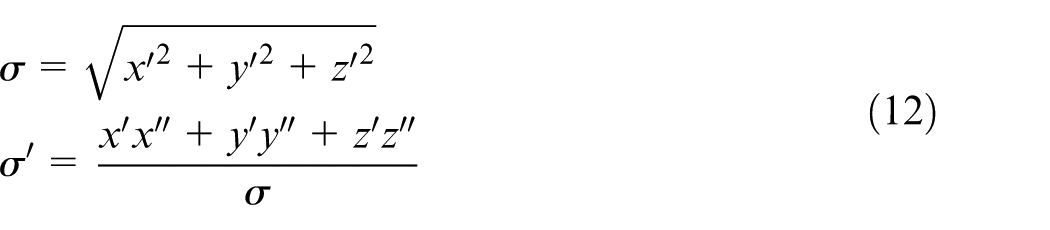
For most of the parametric curves, its relationship between the arc length s and curve parameter u is not analysis but its arc differential can be obtained. The arc differential of the parametric spline can be expressed as follows
The length between u0 and ui can be expressed as follows
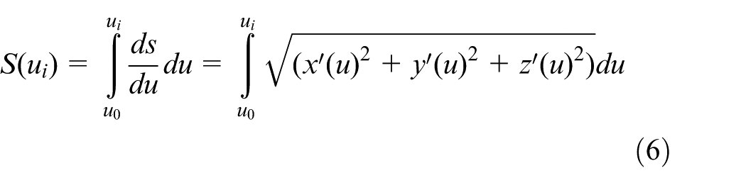
Generally, equation (6) is calculated numerically within a specific tolerance. In this article, the Gauss integration method is used to calculate the arc length for its high precision and calculation efficiency. The Gauss integration with n nodes can be expressed as
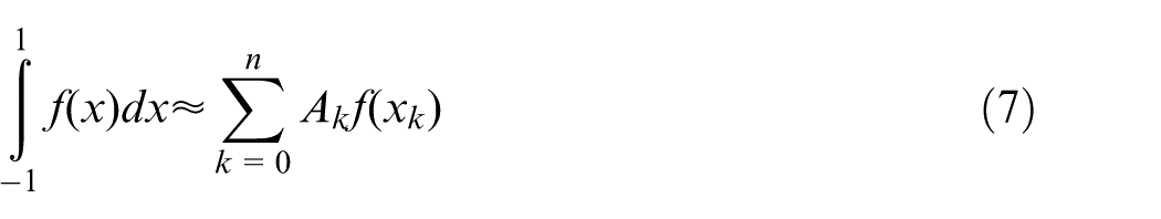
where the value of node xk and weight factor Ak are constant value for a determined n. Here, let n = 3, x1 = −0.7745967, x2 = 0, x3 = 0.7745967, and correspondingly A1 = 0.555556, A2 = 0.888889, and A3 = 0.555556. When the interval range is [a, b], then the Gauss integration is expressed as
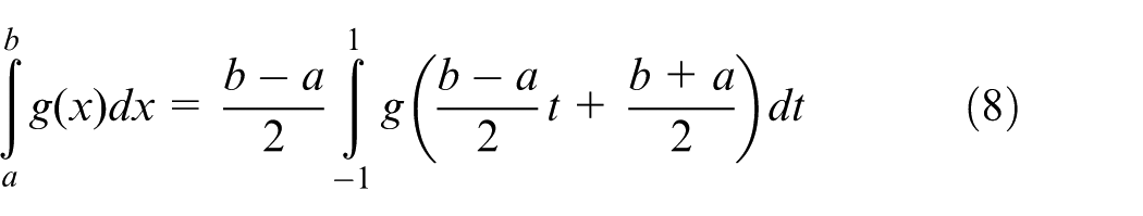
Let
In order to produce the proper curve parameter and arc length pairs (ui, si), a progression calculation process is applied. As indicated earlier, these points are used in fitting u-s B-spline. The progression calculation process is executed by following:
Step 1. A start interval
Step 2. If ui+1 ⩾ 1, let ui+1 = 1. The arc length for the parameter interval range [ui, ui+1] is calculated by
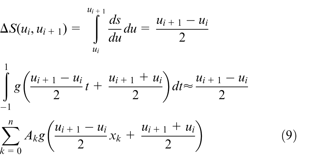
Step 3. The interval [ui, ui+1] is split into two equal sized intervals, denoted as [ui, ui0] and [ui0, ui+1] and Gauss integration is applied on both subintervals to obtain the lengths
Step 4. Determine whether a given tolerance of
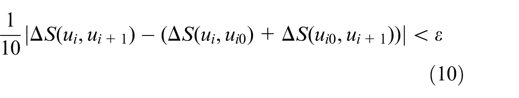
Note that if equation (10) is satisfied, then the approximation is within the given tolerance of the true arc length.
Step 5. If equation (10) is not satisfied, then ui+1 = ui0, then go to step 2.
Step 6. If equation (10) is satisfied, then si+1 = si + ΔS(ui, ui0) si+2 = si+1 + ΔS(ui0, ui+1) and ui+2 = ui+1, ui+1 = ui0. If ui+2 equals to 1, then go to step 8.
Step 7. Let i = i + 2, ui+1 = ui + 2(ui − ui − 2), then go to step 2.
Step 8. A series sample data points (ui, si) are obtained. Then, the vector of curve parameters

Dividing the (s i , u i ) sampled data points
As shown in Figure 2, the second derivative of the cubic basis function is continuous. According to equation (4), the fitted s-u curve is also satisfied that the second derivative
where
So, the sampled data points (si, ui) can be divided in the point where its second derivative
Fit the s-u cubic B-spline in each segment
In approximation process, a feedrate fluctuation bound, E, is proposed along with the sample data (si, ui) to be fitted
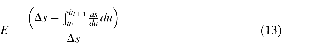
where
As shown in equation (4), the number of control points n required to obtain the desired feedrate fluctuation is usually not known in advance. Hence, the approximation process is generally iterative. The approximate method proceeds as follows:
Step 1. Start with the minimum number of the control points;
Step 2. Fit an approximating curve to the data using a global fit method;
Step 3. Check the feedrate fluctuation of the fitted s-u cubic B-spline;
Step 4. If they satisfy the error requirements, return; otherwise, increase the number of the control points and go back to Step 2.
In each iteration process, the basis function and the control points should be obtained after the number of the control points is determined. To avoid the nonlinear problem, the knots vector is precomputed and the unknown control points are obtained by solving the optimal problem under derivative constraints.
Determining the knot vector of the s-u cubic B-spline
After the number of the control points is determined, the number of the knot vector elements is also obtained. The knot vector VS can be defined as follows
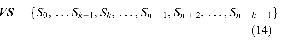
The basis function of equation (4) is constructed by the knots vector and the elements of the knot vector should be determined. According to Figure 2, the third derivative of the basis function is discontinuous in the entire cubic B-spline and it is constant in every knot span. Therefore, the knot elements can be distributed according to the third derivative of the curve parameter respect to the arc length
Optimizing the control points of the s-u cubic B-spline
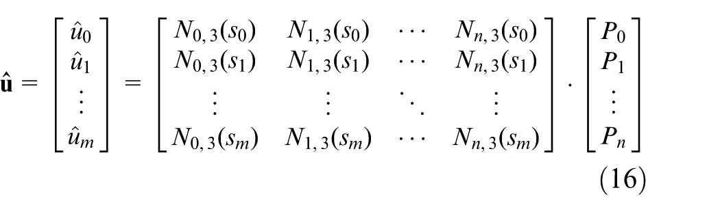
After the knot vector VS is obtained, the basis function of the s-u cubic B-spline as shown in equation (4) is determined. Then, the control points of the s-u cubic B-spline can be obtained by applying a least-squares fit method over the arc length and curve parameter values (

For the arc length vector
Let

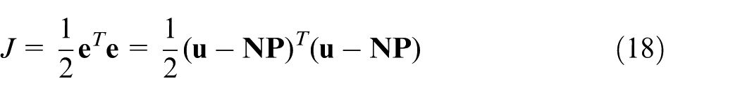
The objective function to be minimized is
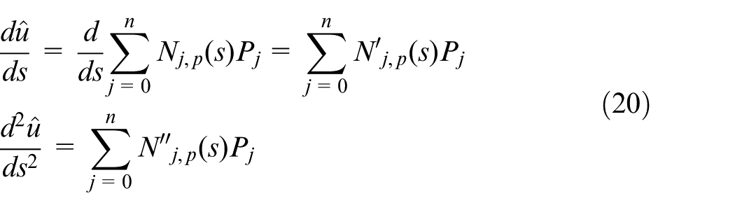
For any parametric curve, its first and second derivatives of the curve parameter with respect to the arc length can be obtained as
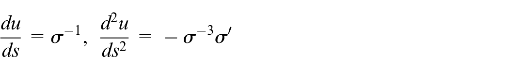
where

The predicted first and second derivatives are obtained as
In order to maintain the fitted s-u cubic B-spline pass through the start point (s,u) start and end point (s,u) end , then

According to equations (20) and (21), the equality constraints can be written as
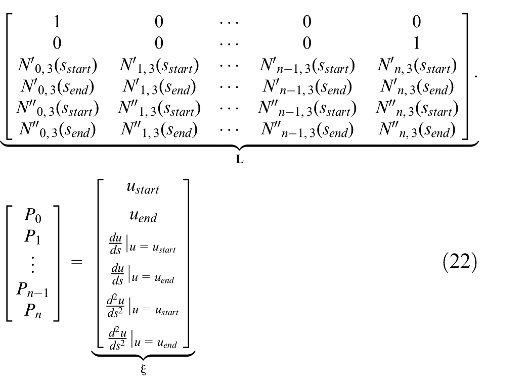
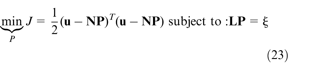
Hence, the control points of the s-u cubic B-spline are obtained by solving the optimization problem
By introducing the vector of Lagrange multipliers
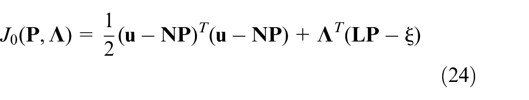
Then, the linear equation can be yielded by equating the partial derivatives to zero, that is,
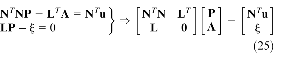
The linear equation (25) has full rank when the segment arc length is nonzero.
Compositing all the s-u B-spline
After each s-u sample data segment is fitted, those divided B-splines are still inconvenient for the parametric interpolation. As the s-u sample data are continuous, they can be composited to a whole cubic B-spline. The fitted s-u B-spline in the ith segment is
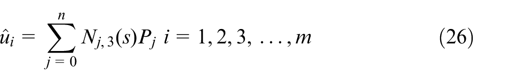
where m is number of the divided s-u sample data according to section “Dividing the (si, ui) sampled data points.”
1. Determine the control points Pj
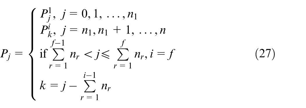
where
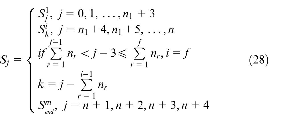
2. Determine the knot vector
Simulations
As shown in Figure 4, two parametric curves are applied to verify the robustness and the accuracy of the proposed OFB method. For the feedrate has great influence in the accuracy of the interpolation, the feedrate scheduled for those curves is shown in Figure 5. Compared with the proposed OFB method, the commonly used OE interpolation methods, for example, the first- and second-order Taylor methods are also applied.
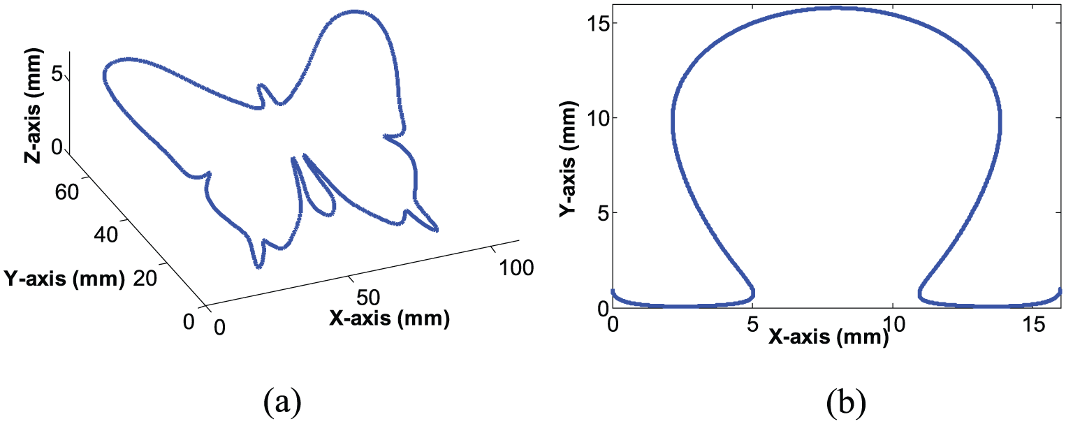
The parametric curves for simulation: (a) the three-dimensional curve and (b) the two-dimensional curve.
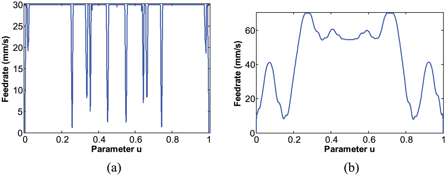
The scheduled feedrate profile: (a) the scheduled feedrate profile for 3D curve and (b) the scheduled feedrate profile for 2D curve.
The feedrate fluctuation proposed in equation (13) is present as a criterion to verify the accuracy of the interpolator. As shown in Figure 6, the first-order Taylor method has poor feedrate fluctuation even the feedrate is scheduled in the sharp corners. Compared with the first-order Taylor method, the feedrate fluctuation of the second-order Taylor method in Figure 7 is eliminated. For a given feedrate fluctuation requirement E = 0.05%, the feedrate fluctuation of the proposed OFB method in Figure 8 satisfies the error requirement and its feedrate fluctuation can be further eliminated by increasing the number of the control points. The feedrate fluctuation is summarized in Table 1 and the accuracy of the proposed OFB method is demonstrated. As shown in Table 1, the feedrate fluctuation is decreased by about 50% compared with the second-order Taylor method and is about 3% of the first-order Taylor method when the feedrate is scheduled for the three-dimensional (3D) curve. For the two-dimensional (2D) curve, the feedrate fluctuation is about 3% of the first-order Taylor method when the feedrate is scheduled.
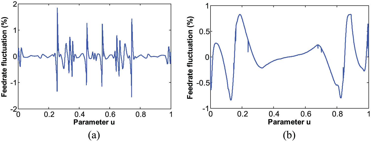
The feedrate fluctuation of the first-order Taylor interpolation method after the feedrate is scheduled: (a) the result of the 3D curve and (b) the result of the 2D curve.
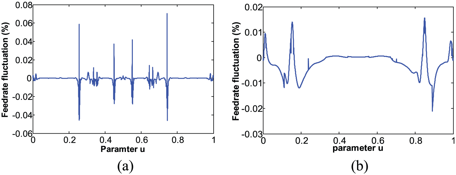
The feedrate fluctuation of the second-order Taylor interpolation method after the feedrate is scheduled: (a) the result of the 3D curve and (b) the result of the 2D curve.
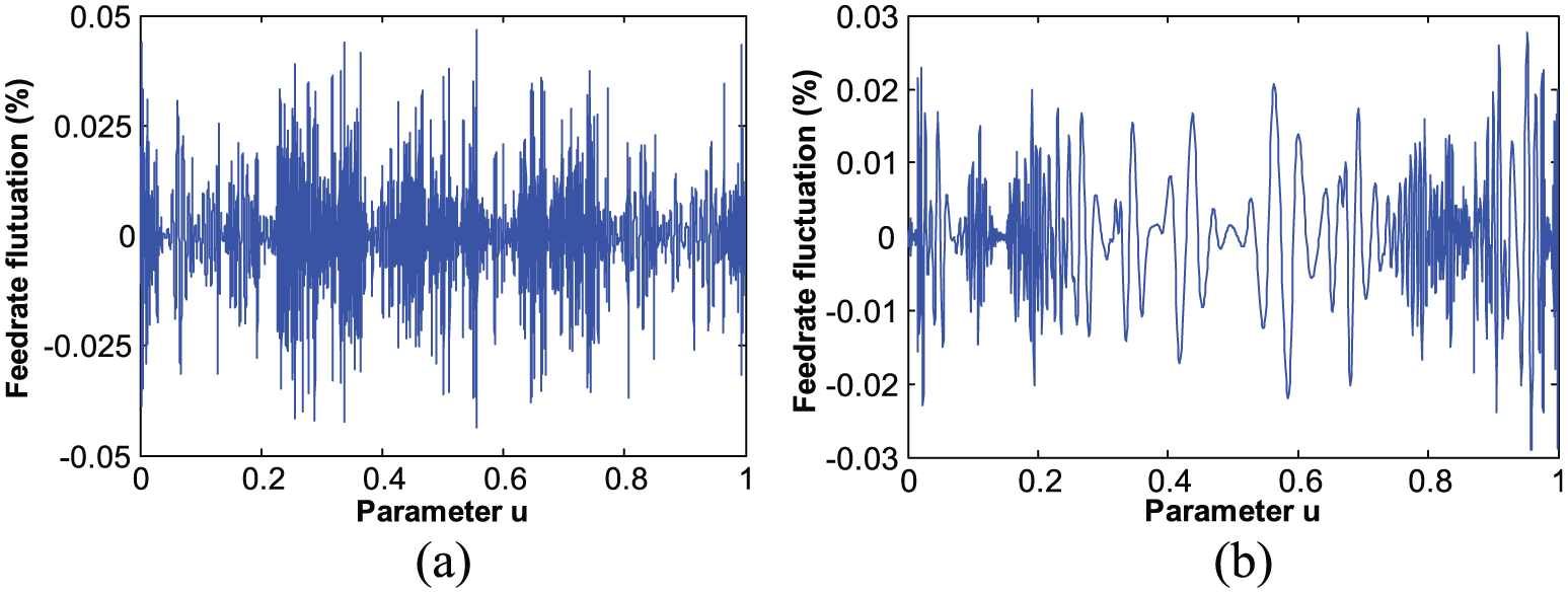
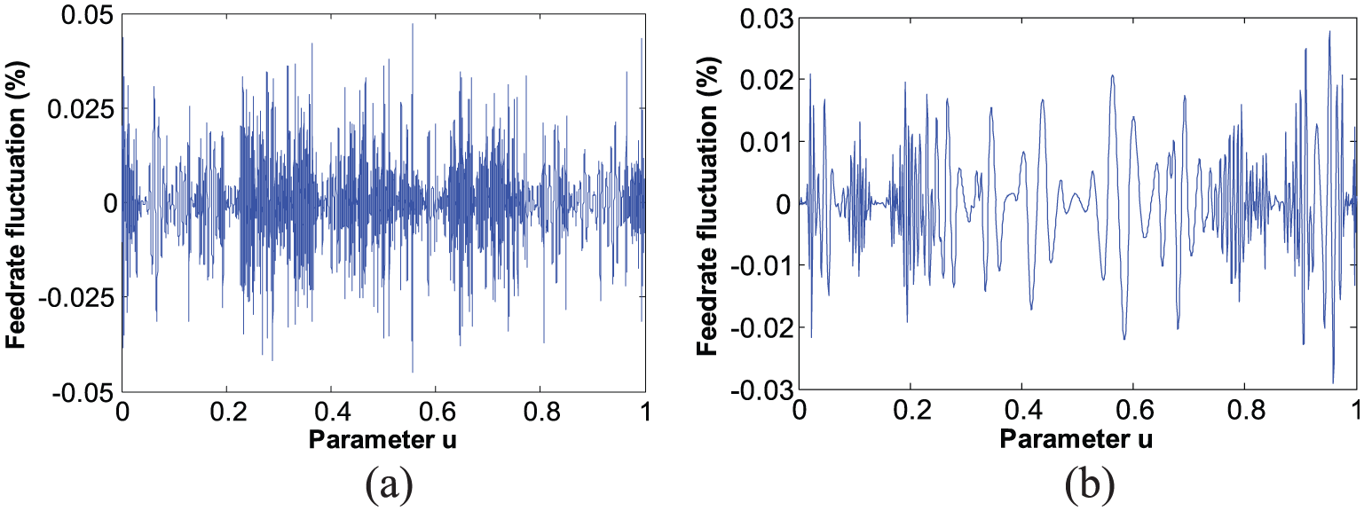
The feedrate fluctuation of the proposed OFB interpolation method after the feedrate is scheduled: (a) the result of the 3D curve and (b) the result of the 2D curve.
Maximum absolute feedrate fluctuation (%).
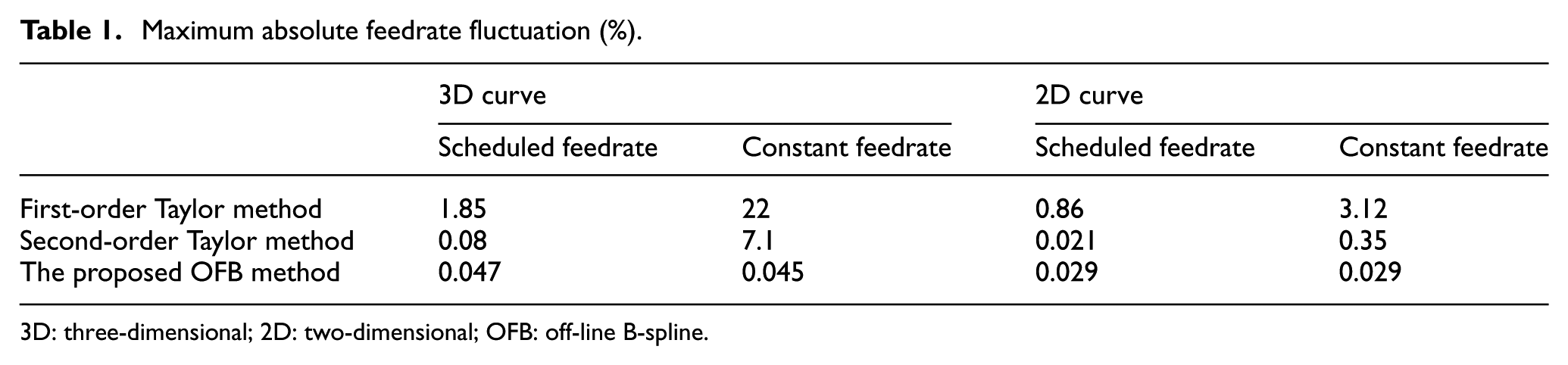
3D: three-dimensional; 2D: two-dimensional; OFB: off-line B-spline.
In order to verify the robustness of the OFB interpolation method, constant feedrate 25 mm/s is applied to the three interpolation methods in the same curves. As shown in Figures 9 and 10, the first- and second-order interpolation methods have great feedrate fluctuation even though the feedrate is 25 mm/s in common curves. So the OE interpolation is not suitable for high speed and precision manufacture due to the low robustness. The feedrate fluctuation of the OFB method in constant feedrate 25 mm/s is shown in Figure 11 and the feedrate fluctuation still satisfies the error requirements E = 0.05% even in the sharp corners. As shown in Table 1, the feedrate fluctuation of the OFB method is less than 1% of the OE method when the feedrate is constant.
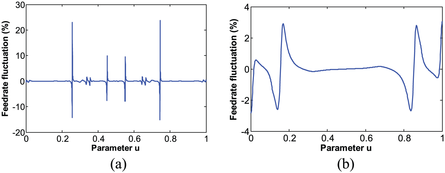
The feedrate fluctuation of the first-order Taylor interpolation method at the feedrate of 25 mm/s: (a) the result of the 3D curve and (b) the result of the 2D curve.
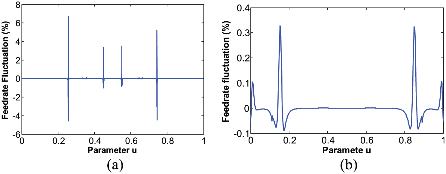
The feedrate fluctuation of the second-order Taylor interpolation method at the feedrate of 25 mm/s: (a) the result of the 3D curve and (b) the result of the 2D curve.
The feedrate fluctuation of the proposed OFB interpolation method at the feedrate of 25 mm/s: (a) the result of the 3D curve and (b) the result of the 2D curve.
In modern manufacture controller, more and more intelligent modules such as thermal compensation module and real-time interference checking module are embedded in. The real-time computation resources become more precious. For OE method, the accuracy and computing efficiency always contradict. In order to obtain high accuracy, complex derivative and iteration calculation in OE method, which means low computing efficiency, is always required. But in the proposed method, the s-u cubic B-spline can be calculated by de Boor method effectively. The arithmetic operations required for different methods are shown in Table 2. As shown in Table 2, the arithmetic operations of the proposed OFB method are much less than the first- and second-order method. As shown in Table 2, the computation load of the proposed method is decreased by about 70% compared with the second-order interpolation method and about 60% compared with the first-order interpolation method.
Arithmetic operations required for different real-time interpolation methods.
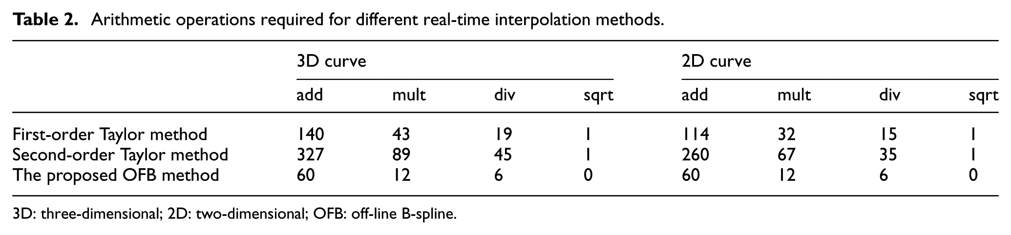
3D: three-dimensional; 2D: two-dimensional; OFB: off-line B-spline.
Experiments
In order to verify the proposed OFB interpolation method, the experiments are carried out. The tool path is shown in Figure 4. The experiment platform is a PC-based open computer numerical control (CNC) (A3200) machine developed by Aerotech. The A3200 controller is performed on the industrial computer with the real-time extension, RTX, embedded in Windows XP and the A3200 controller also provides the lowest level to the position and velocity commands sent to the drives in real time. Then, the proposed OFB interpolator is designed on the open motion controller for our own purpose and the interpolator period is chosen as 1 ms. The translational axes of the platform are driven by the linear motors and the moving bodies are separated by air bearing, so the stiffness of machine is low. For safety consideration, the material of the workpiece is paraffin. The experimental result of the tool path trajectory is shown in Figure 12. The experimental result shows that the proposed OFB interpolation method is feasible and applicable.
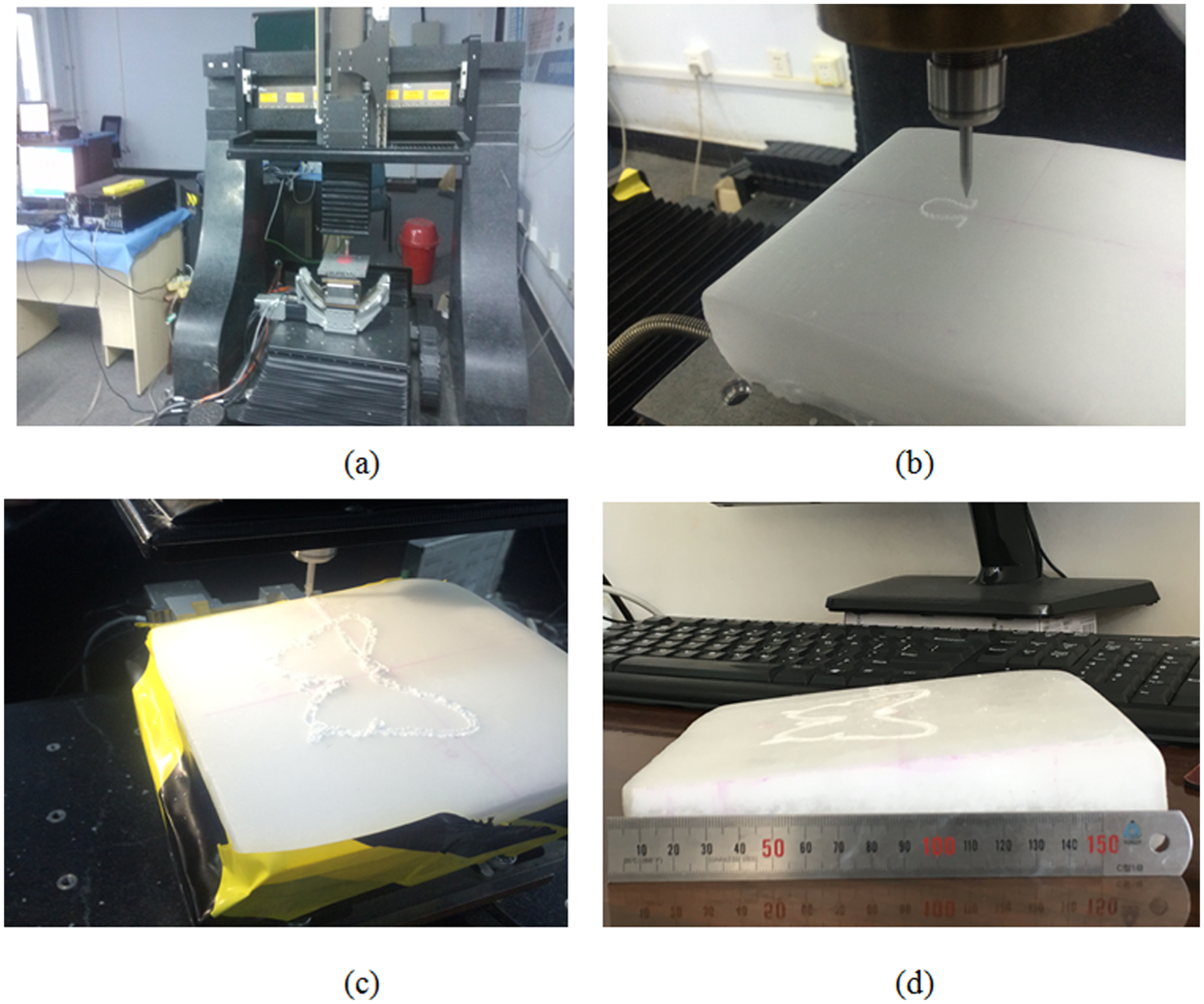
The experimental results: (a) the five-axis polishing machine tool, (b) the 2D machine result by the proposed OFB method, (c), (d) the 3D machine result by the proposed OFB method.
Conclusion
As the requirements of the accuracy, robustness, and computation load of the manufacture process increase, the off-line fitting method interpolation is widely applied especially in high precision and complex free-form surface manufacturing. Compared with the existing polynomial-fitting interpolation method, a cubic B-spline fitting method (OFB) is proposed. For the locality and flexibility of the B-spline, the required feedrate fluctuation of 0.05% is more easily satisfied. The real-time computing consumption of the OF interpolation method is less than that of the OE method, for most of the computations are performed in the off-line process. First, the sampled s-u data points are obtained by adaptive Gauss integration and those sampled points are divided according to the third derivative of the curve parameter with respect to the arc length. In each segment, the proper cubic B-spline is fitted according to the sampled data points by constant iterative. Finally, the fitted s-u cubic B-spline is embedded into the NC code for real-time interpolation. Compared with the second-order interpolation method, the feedrate fluctuation is decreased by about 50% when the feedrate is scheduled and the feedrate fluctuation is about 3% of the second-order interpolation method when the feedrate is constant for the complex 3D curves. The real-time calculation consumption of the proposed OFB method is decreased by about 70% compared with the OE method. The accuracy, robustness, and computation efficiency are demonstrated by the simulation analysis and the experiments verify that the OFB interpolation method can realize high-accuracy complex free-form machining successfully.
Footnotes
Declaration of conflicting interests
The author(s) declared no potential conflicts of interest with respect to the research, authorship, and/or publication of this article.
Funding
The author(s) disclosed receipt of the following financial support for the research, authorship, and/or publication of this article: The authors are grateful for the financial support from the National High Technology Research and Development Program (863 Program) of China (Grant No. 2012AA041304).