Nonanthropomorphic exoskeleton with legs based on eight-bar linkages

Abstract

This article presents the principles upon which a new nonanthropomorphic biped exoskeleton was designed, whose legs are based on an eight-bar mechanism. The main function of the exoskeleton is to assist people who have difficulty walking. Every leg is based on the planar Peaucellier–Lipkin mechanism, which is a one degree of freedom linkage. To be used as a robotic leg, the Peaucellier–Lipkin mechanism was modified by including two more degrees of freedom, as well as by the addition of a mechanical system based on toothed pulleys and timing belts that provides balance and stability to the user. The use of the Peaucellier–Lipkin mechanism, its transformation from one to three degrees of freedom, and the incorporation of the stability system are the main innovations and contributions of this novel nonanthropomorphic exoskeleton. Its mobility and performance are also presented herein, through forward and inverse kinematics, together with its application in carrying out the translation movement of the robotic foot along paths with the imposition of motion laws based on polynomial functions of time.

Introduction

An exoskeleton is a wearable passive or active device, intended to extend and enhance user capability. It also complements or substitutes certain human functions. ¹ Passive exoskeletons of lower limbs are commonly referred to as orthotic devices, with the user applying force to move the limb. In active exoskeletons, actuators on the machine move the leg. ² The history of the design and development of exoskeletons began in the 1960s, when the US army developed a great variety of equipment to increase the ability of soldiers to fulfill their military functions. Later, new applications were given to exoskeletons that included protection and armor for handling radioactive or hazardous materials and the rehabilitation of seriously injured elbows and knees. ^3,4 As an assistive technology, exoskeletons found revolutionary applications concerning human quality of life. Scientific research efforts have focused on the rehabilitation of the lower extremities ⁵ and in recent years, researchers have been looking for ways to assist people that have suffered various degrees of lower limb mobility loss. Because the simple act of walking activates the nerve terminals in the lower limbs, creating the necessary feedback to train the spinal cord, the benefits offered by assistive exoskeletons are undeniable. ^{6 –9}

Most walking exoskeletons are devices designed from traditional mechanical architectures composed of links coupled by either revolute or prismatic joints forming serial chains. These traditional anthropomorphic architectures basically consist of four links, representing the pelvis, femur, tibia, and foot.

However, other architectures present several advantages. A novel wearable robot with a nonanthropomorphic architecture, intended to assist hip and knee flexion/extension, is presented by Accoto et al. ¹⁰ and Sergi et al. ¹¹ The authors explain that this architecture helps to improve ergonomics and optimizes dynamic properties through an intelligent distribution of swinging masses. The resulting wearable robot shows low reflected inertia, high backdrivability, and intrinsic misalignment tolerance.

Sergi ¹² discusses the use of anthropomorphic and nonanthropomorphic wearable robots. On the one hand, the author addresses the issue concerning the intrinsic problems that arise when dealing with anthropomorphic architectures, affirming that the kinematic compatibility between the robotic structure and the user must be guaranteed. The two mechanical systems have to be identical. He states that the problem is defining the exact location and orientation of human joint axes of rotation. In addition, high torques are needed to move those links. ^13,14 On the other hand, Sergi et al. ¹¹ address nonanthropomorphic wearable robots improve ergonomics and performance, due to their intrinsic dynamic properties.

There are several good examples of anthropomorphic exoskeletons. One is the hybrid assistive limb exoskeleton, created by Cyberdyne Inc (Tsukuba, Japan), which represents the latest generation in assistive mechanical exoskeletons. ¹⁵ Another is the Berkeley lower extremity exoskeleton wearable robot, which includes two powered anthropomorphic legs, a power supply, and a backpack-like frame on which heavy payloads can be mounted. ¹⁶ Berkeley Bionics and the University of California at Berkeley developed the eLEGS biped exoskeleton, which is a mobile wearable robot used by patients suffering from spinal cord injuries. ¹⁷

Aim and scope

In the present article, we propose a nontraditional mechanical architecture, arranged in a nonanthropomorphic structure. It is based on the planar Peaucellier–Lipkin (PL) linkage, which has been modified by the addition of two more degrees of freedom (DOFs). Figure 1 shows the PL-based exoskeleton and the initial prototype is shown in Figure 2. We describe the principles upon which this wearable robot has been created and the transformation the basic PL mechanism has undergone at the different stages of the mechanical design process. The detailed design and attributes are found by Juarez et al. ¹⁸

Figure 1.

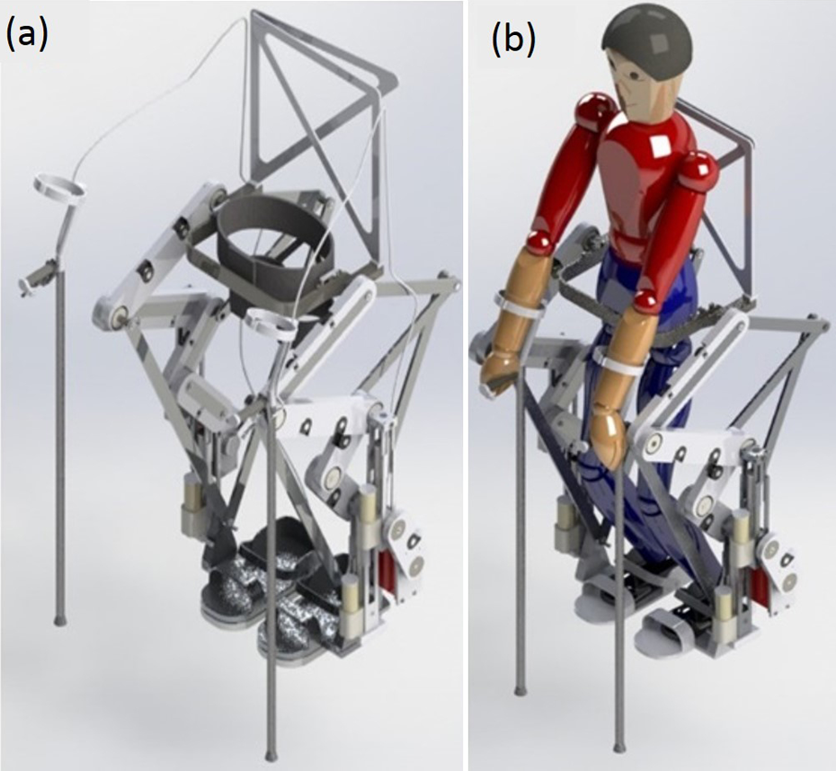
Exoskeleton model based on the PL mechanism (a) without and (b) with a user. PL: Peaucellier–Lipkin.

Figure 2.

Prototype of the PL-based exoskeleton in construction. PL: Peaucellier–Lipkin.

Mobility is one of the most important criteria for evaluating the performance of an exoskeleton, as are weight and stiffness. Therefore, we present herein direct and inverse kinematics, which are tested by tracking two paths governed by two time laws. We focus on the smoothness of motion in relation to function continuity at the path points. On the one hand, we evaluate its mobility by generating a trajectory that is nonreal for human gaits. It is formed by three curves, tangentially connected, and governed by a segmented time function. On the other hand, we consider a trajectory generated by the ankle of a person executing a normal gait.

Description of the nonanthropomorphic exoskeleton leg

The PL linkage has found several applications; Khandelwal et al. ¹⁹ present its use in a linear haptic device. The PL mechanism has been used as a positioning device of teleoperated needle steering systems ²⁰ and as an actuation mechanism of deployable structures, ²¹ among others. However, its use as a wearable robotic leg is nonexistent.

There appears to be scant use of the PL mechanism as a locomotion device in walking machines. Núñez Altamirano et al. ²² present a reptilian five-DOF robotic leg, based on the PL mechanism. It adapts its leg according to a center of rotation, obtained by three points on the path. Due to the ability of the PL mechanism to trace defined paths, including straight lines or circular arcs, ^23,24 the end effector of the five-DOF robotic leg moves parallel to the edge of the road. Núñez Altamirano et al. ²⁵ provide the dynamics of the same robotic leg presented by Núñez Altamirano et al., ²² when it executes a walking gait along a straight line in the transfer phase. The reptilian robotic leg, discussed by Núñez Altamirano et al., ^22,25 is used as a locomotion limb in n-legged walking machines, when $n=4, 6, \text{\hspace{0.17em}or} 8$ .

The PL mechanism, shown in Figure 3, is composed of eight articulated bars connected by six revolute joints, denoted by points A, B, C, D, E, and F, and whose joint axes are orthogonal to the plane formed by those six points. Considering that lengths of links are denoted by L_jk, where j and k are two of those points, the PL mechanism is composed of three sets of links: $\left\{L_{AD}, L_{AE}\right\},\left\{L_{CD}, L_{CE},L_{DF},L_{EF}\right\},\text{ and }\left\{L_{AB}, L_{BC}\right\}$ , restricted to the conditions given in Table 1.

Figure 3.

(a) Rigid links AB and BC form the basic PL mechanism. (b) Variable links in the transformed mechanism. AB and BC change their lengths as necessary. PL: Peaucellier–Lipkin.

Table 1.

Set of link lengths and conditions.

Set of lengths	Condition
$\left\{L_{AD}, L_{AE}\right\}$	$L_{AD}=L_{AE}=L_1$
$\left\{L_{CD}, L_{CE},L_{DF},L_{EF}\right\}$	$L_{CD}=L_{CE}=L_{DF}=L_{EF}=L_2$
$\left\{L_{AB}, L_{BC}\right\}$	$L_{AB}=L_{BC}$
$L_1>L_{AB}+L_{BC}$

Figure 3(a) shows that point F traces a true straight line, as a result of a rotation motion of the input link BC, given by joint variable θ, with respect to the fixed link AB. This final movement is limited by the length of the bars forming the mechanism. ^{26 –30}

To mimic the human gait, the PL mechanism has been modified with the inclusion of two more DOFs. In other words, the former one-DOF PL mechanism has been transformed into a three-DOF exoskeleton leg. This article shows how it has been modified and consequently presents the forward and inverse kinematics, considering the joint variables denoted by L_AB, L_BC, and θ. The position of the foot is obtained in terms of the coordinates of a specific path and linked to polynomial functions of time.

Conceptual design

To reproduce the human gait with the use of a PL-based exoskeleton, it is important to understand that the human gait is a cyclic motion process, characterized by a single support (SS) phase (one foot in contact with the ground) and a double support (DS) phase (two feet on the ground). As shown in Figure 4, the DS phase represents 20% of the total cycle. For each leg, the step is composed of a support phase, representing 60% of the total duration, and an oscillation phase lasting 40% of the total time. ^{31 –34}

Figure 4.

Gait cycle duration, RF, and LF. RF: right foot; LF: left foot.

Thus, four stages are defined in a normal human gait as follows:

double support stage, both feet touching the ground;

lifting stage, one foot starts rising, leaving the other foot as support;

oscillation stage, one foot moves in the air and the other one continues as support;

descent stage, the oscillating foot begins to descend and the other foot still remains as support; and

the sequence is repeated with the other foot.

Due to the nature of the basic eight-bar PL mechanism, it can only perform linear displacements when $L_{AB}=L_{BC}$ . However, the inclusion of two more DOFs enables the resulting robotic leg to execute each of the four stages mentioned above.

The main modifications exerted on the PL mechanism take the rigid bars AB and BC into account, which are replaced by elements of virtual length, as shown in Figure 3. Rigid bars are represented by solid lines (Figure 3(a)), whereas nonrigid elements are drawn in dashed style (Figure 3(b)). In this manner, variable lengths found between points A and B and between points B and C are the new DOFs and are represented by linear actuators, driving two prismatic joints.

We now introduce the pelvis and foot links, which are shown in Figure 5. The first one is joined at F, whereas the second one is positioned at A, firmly fixed to link AB. It is important to note that point A represents the robotic ankle. As shown in Figure 5, the pelvis link can freely rotate an angle μ around an axis passing at point F, orthogonal to the plane formed by points A to F. Considering that the user’s hip is placed at and fixed to this link, it is imperative that the exoskeleton pelvis or hip not rotates freely. Thus, the hip should always maintain the same orientation, avoiding being swung by the user.

Figure 5.

The addition of the pelvis and foot.

To overcome this problematic condition, we introduce an orthogonal stability system (OSS), which prevents this angular fluctuation. The OSS works as a parallelogram mechanism and is a type of four-bar linkage, whose opposite sides have the same lengths and remain parallel to each other. The OSS enables the pelvis to undergo constant orientation at any time, referred to link AB. It is important to note that link AB is fixed to the robotic foot, which is posed on the horizontal ground. That is to say, link AB is always orthogonal to the ground.

Figure 6 shows the OSS, which is composed of several toothed pulleys and timing belts.

Figure 6.

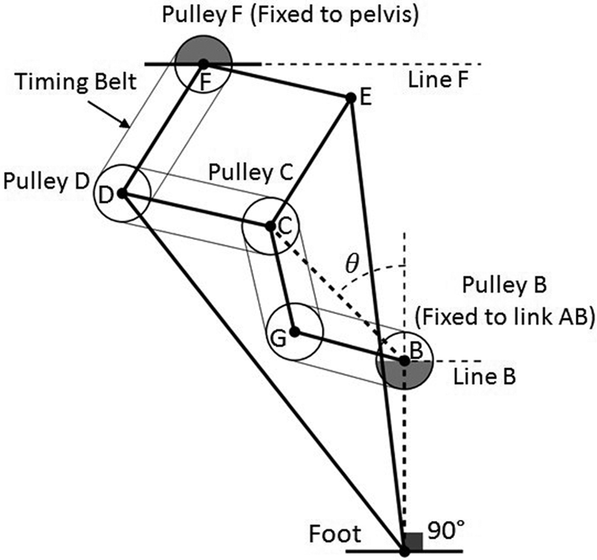
OSS attaches the pelvis to link AB. As a consequence, line F, representing the orientation of the pelvis, is always parallel to line B, which is always horizontal. OSS: orthogonal stability system.

Pulleys are placed at points B, G, C, D, and F. The first and last pulleys are fixed to link AB and the pelvis, respectively, whereas the others can rotate freely around their own axes. Because link BC has variable length, it is not possible to introduce a timing belt between points B and C; consequently, there is a pulley placed at an extra point, denoted by G, and supported by two extra links, connecting points BG and CG. Those two links do not offer support to the total weight of the exoskeleton and user. Their function is strictly to support pulley G and keep the timing belts tight. Consequently, points B, C, and G form a deployable triangle with sides BG and CG and are constant at any time. The length of side BC increases or decreases as required during gait.

Figure 7 presents the exoskeleton, whose legs are based on the modified PL mechanism. Its right foot is in the support or contact phase, because it touches the ground, whereas the left foot oscillates in the air or in the flight phase. The walking gait is obtained when L_AB, L_BC, and θ coordinately evolve. See the arrows in Figure 7.

Figure 7.

Exoskeleton legs driven by two linear actuators and a rotary actuator at B.

The inclusion of two more DOFs and the OSS results in a new mechanism that has the ability to draw more complex paths, allowing the PL-based exoskeleton, with a nonanthropomorphic architecture, to walk in an anthropomorphic manner.

Mathematical analysis

Each PL-based leg has three DOFs, which are capable of transforming the entire linkage; they are L_AB, L_BC, and θ, and the main behavior of the PL-based leg depends on them, according to the next five cases

• Case 1 occurs when $L_{AB}=L_{BC}=K_1$ and θ varies; point F₁ draws a straight line (see Figure 8), where the PL mechanism involved corresponds to subscript 1.

• Case 2 happens when $L_{AB}<L_{BC}$ and θ evolves; point F₂ traces a concave circular arc, with the perspective of an observer placed at A (see Figure 8), and note the PL mechanism corresponds to subscript 2.

• Case 3 takes place once $L_{AB}>L_{BC}$ and θ changes; point F₃ describes a convex circular arc, when an observer is positioned at A (see Figure 8), and consider the mechanism denoted by subscript 3.

• Case 4 refers to $L_{AB}=L_{BC}=K_4,\text{ where }{K}_4>K_1$ , as shown in Figure 9(a). Under this condition, point F₄ draws a straight line, as in case 1. Nevertheless, the shortest distance between point A and the line traced by point F₄ is shorter than the one concerning case 1, as shown in Figure 9(b). It is important to note that the shortest distance between point A and the line traced by point F₄ corresponds to the length of the line that is the common perpendicular between the axis at A and the line traced by point F₄. Subscript 4 helps to identify the PL mechanism concerning case 4. Lines traced by F₁ and F₄ are separated by Δ₄.

• Case 5 $L_{AB}=L_{BC}=K_5,\text{ where }{K}_5<K_1$ . Under this condition, point F₅ draws a straight line, as in case 1. However, the shortest distance between point A and the line traced by point F₅ is larger than the one concerning case 1 (see Figure 9(c)). Lines traced by F₁ and F₅ are separated by Δ₅.

Figure 8.

PL mechanism in cases 1, 2, and 3 corresponding to subscripts 1, 2, and 3, respectively. PL: Peaucellier–Lipkin.

Figure 9.

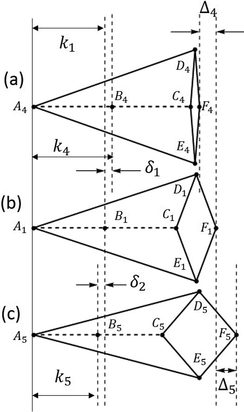
PL in cases 1, 4, and 5, where subscripts 1, 4, and 5 help to identify them. PL: Peaucellier–Lipkin.

Through these five cases, we can understand that each PL-based leg is able to trace complex paths, including the one followed by a human foot, during gait.

Forward kinematics

Let $\Theta ={\left(\begin{array}{ccc}{L}_{AB}& L_{BC}& \theta \end{array}\right)}^T\in {\mathcal{R}}^3$ be called the joint space, and let ${\mathfrak{X}}_{\text{A}}={\left(\begin{array}{cc}{A}_{X_j}& A_{Y_j}\end{array}\right)}^T\in {\mathcal{R}}^2\text{ and }{\mathfrak{X}}_{\text{F}}={\left(\begin{array}{cc}{A}_{F_j}& A_{F_j}\end{array}\right)}^T\in {\mathcal{R}}^2$ be called the task space, defining the vectors describing points A and F, respectively, with respect to the frame $\left\{j\right\},\text{ where }j=0\text{ or }j=F$ . Forward kinematics consists of finding ${\mathfrak{X}}_{\text{A}}=\mathcal{F}\left(\Theta \right)\text{ and }{\mathfrak{X}}_{\text{F}}=\mathcal{G}\left(\Theta \right)$ .

To calculate ${\mathfrak{X}}_{\text{A}}=\mathcal{F}\left(\Theta \right)\text{ and }{\mathfrak{X}}_{\text{F}}=\mathcal{G}\left(\Theta \right)$ , it is necessary to describe frames $\left\{0\right\}=\left\{{\widehat{x}}_0, {\widehat{y}}_0, {\widehat{z}}_0\right\}\text{ and }\left\{F\right\}=\left\{{\widehat{x}}_F, {\widehat{y}}_F, {\widehat{z}}_F\right\}$ , which appear in Figure 10. Note that the origin of frame {0} and A match, whereas the origin of the reference system {F} and F coincide. Vector ${\widehat{y}}_0$ coincides with bar AB, directed from A to B. Vector ${\widehat{z}}_0$ is orthogonal to the plane formed by points A, B, C, D, and F and ${\widehat{x}}_0={\widehat{y}}_0\otimes {\widehat{z}}_0$ . Frame {F} is described in terms of {0}, as shown below

${}_{}{}^0\left\{F\right\}=\left\{I_{3x3}; {\left(\begin{array}{ccc}{F}_{X_0}& F_{X_0}& 0\end{array}\right)}^T\right\}$

1

Figure 10.

Geometry concerning the PL linkage. PL: Peaucellier–Lipkin.

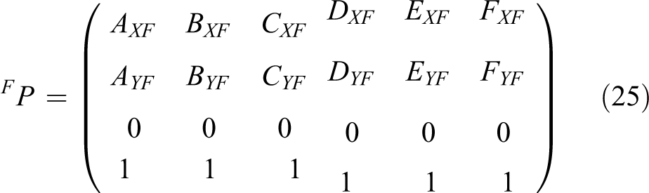
According to the geometry given in Figure 10, coordinates of points A and F, as well as B, C, D, and E, referred to {0}, are denoted by equations (2) to (13).

$A_{X_0}=0$

2

$A_{Y_0}=0$

3

$B_{X_0}=0$

4

$B_{Y_0}=L_{AB}$

5

$C_{X_0}=-L_{BC}S\theta$

6

$C_{Y_0}=L_{AB}+L_{BC}C\theta$

7

$D_{X_0}=L_{AD}S{\epsilon }_1$

8

$D_{Y_0}=L_{AD}C{\epsilon }_1$

9

$E_{X_0}=L_{AE}S{\epsilon }_2$

10

$E_{Y_0}=L_{AE}C{\epsilon }_2$

11

$F_{X_0}=d_{AF}S\alpha$

12

$F_{Y_0}=d_{AF}C\alpha$

13

where C and S mean cosine and sine functions, respectively, and

${∊}_1=\alpha +\beta$

14

$\alpha ={\text{Tan}}^{-1}\left(\frac{-L_{BC}S\theta }{L_{AB}+L_{BC}C\theta }\right)$

15

$\beta =C^{-1}\left(\frac{L_{AD}^2+d_{AC}^2-L_{CD}^2}{2 L_{AD}{d}_{AC}}\right)$

16

$d_{AC}=\sqrt{{\left(L_{AB}+L_{BC}C\theta \right)}^2+{\left(L_{BC}S\theta \right)}^2}$

17

${\epsilon }_2=\alpha -\beta$

18

$d_{AF}=d_{\text{AMR}}+d_{\text{CMR}}$

19

$d_{\text{AMR}}=L_{AD}C\beta$

20

$d_{\text{CMR}}=d_{\text{AMR}}-d_{AC}$

21

Points given by equations (2) to (13) are referred to {0}, but under certain conditions, they could be described with respect to {F}. In this case, it is necessary to transform them with the use of equation (22), where ${}_{}{}^{0}P\text{ and }{}_{}{}^{F}P$ are two point clouds collecting coordinates of points A, B, C, D, E, and F, referred to {0} and {F}, respectively

${}_{}{}^{F}P={T_F^0}^{-1}{}_{}{}^{0}P$

22

where $T_F^0$ is the homogeneous transformation, which maps a point cloud from {F} to {0}, see equation (23)

$T_F^0=\left(\begin{array}{cc}{I}_{3x3}& \begin{array}{c}{F}_{X_0}\\ F_{Y_0}\\ 0\end{array}\\ {\overline{0}}^T& 1\end{array}\right)$

23

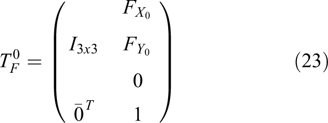
Equation (22) concerns homogeneous point clouds ${}_{}{}^{0}P\text{ and }{}_{}{}^{F}P$ , which are shown below

${}_{}{}^{0}P=\left(\begin{array}{c}\begin{array}{ccc}{A}_{X_0}& B_{X_0}& C_{X_0}\\ A_{y_0}& B_{Y_0}& C_{Y_0}\\ 0& 0& 0\end{array}\\ \begin{array}{ccc}1 & 1 & 1\end{array}\end{array}\begin{array}{c}\begin{array}{ccc}{D}_{X_0}& E_{X_0}& F_{X_0}\\ D_{Y_0}& E_{Y_0}& F_{Y_0}\\ 0& 0& 0\end{array}\\ \begin{array}{ccc}1 & 1 & 1\end{array}\end{array}\right)$

24

${}_{}{}^{F}P=\left(\begin{array}{c}\begin{array}{ccc}{A}_{XF}& B_{XF}& C_{XF}\\ A_{YF}& B_{YF}& C_{YF}\\ 0& 0& 0\end{array}\\ \begin{array}{ccc}1 & 1 & 1\end{array}\end{array}\begin{array}{c}\begin{array}{ccc}{D}_{XF}& E_{XF}& F_{XF}\\ D_{YF}& E_{YF}& F_{YF}\\ 0& 0& 0\end{array}\\ \begin{array}{ccc}1 & 1 & 1\end{array}\end{array}\right)$

25

Inverse kinematics

Considering that (i) the foot link could be placed on the terrain, while the pelvis link could move along a prescribed path, or (ii) the pelvis link could be considered fixed and the foot link could travel, inverse kinematics lets Θ be obtained in terms of ${\mathfrak{X}}_{\text{A}}\text{ or }{\mathfrak{X}}_{\text{F}}$ by means of $\mathcal{H}:{\mathfrak{X}}_{\text{A}}\to \Theta \text{ or }\mathcal{I}:{\mathfrak{X}}_{\text{F}}\to \Theta$ .

Figure 10 describes condition (ii), so {F} is considered fixed, and point A, referred to {F}, moves along a prescribed path. Thus, the inverse kinematics analysis consists of finding $\mathcal{H}:{\mathfrak{X}}_{\text{A}}\to \Theta$ .

According to Figure 10, L_AF, ε_ci, L_AMR, L_AC, and α_ci are obtained by equations (26) to (30)

$L_{AF}=\sqrt{x^2+y^2}$

26

${\epsilon }_{ci}=C^{-1}\left(\frac{L_{AD}^2+L_{AF}^2-L_{DF}^2}{2L_{AD}{L}_{AF}}\right)$

27

$L_{\text{AMR}}=L_{AD}\text{Cos}{\epsilon }_{ci}$

28

$L_{AC}=2 L_{AMR}-L_{AF}$

29

${\alpha }_{ci}=S^{-1}\left(\frac{\left|y\right|}{L_{AF}}\right)$

30

Figure 10 presents the joint variables L_AB, L_BC, and θ. Although L_AB and L_BC can vary independently, this article considers cases 1, 4, and 5, in which $L_{AB}=L_{BC}$ . This means that the number of DOFs is reduced to two. Therefore, the positioning of the exoskeleton foot deals with the description of $L_{AB}=L_{BC}$ and θ in terms of the coordinates of point A, referred to {F}.

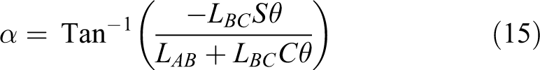
Figure 10 shows the isosceles triangle formed by points A, B, and C, whose equal sides have lengths denoted by L_AB and L_BC. They are described by equations (31) and (32). The side formed between points A and C is defined by equation (29)

$L_{AB}=\frac{L_{AC}{L}_{AF}}{2\left|y\right|}$

31

$L_{BC}=\frac{L_{AC}{L}_{AF}}{2\left|y\right|}$

32

Angle θ is obtained with the aid of equation (34), which depends on equation (33), according to Figure 10

$\phi =C^{-1}\left(\frac{L_{AB}^2+L_{BC}^2-L_{AC}^2}{2L_{AB}{L}_{BC}}\right)$

33

$\theta =\pi -\phi$

34

Inverse kinematics can now be linked to a possible geometric region or path described by parametric coordinates, referred to {F}. ^35,36 Keep in mind that the basic PL mechanism is a planar one, and the addition of two more DOFs does not alter this attribute. Because the plane on which points A, B, C, D, E, and F exist coincides with the one formed by ${\widehat{x}}_F\text{ and }{\widehat{y}}_F$ , only two coordinates are needed.

Simulations

To make the above theoretical framework comprehensible, two simulations are reported herein. In both of them, the legs of the exoskeleton execute a half of a single cycle of the gait and the user’s hip is positioned at a constant height during the travel. According to Lin et al., ³⁷ the human hip does not travel at a constant height during the gait cycle. It oscillates some few centimeters in a sinusoidal manner ³⁸ during a slow travel, as the one performed by the PL-based exoskeleton.

On the one hand, we present the case in which the left robotic leg performs the transfer phase, while the right one executes the support stage. The purpose of this test is to show the advantage of this nonanthropomorphic exoskeleton obtained from the intrinsic nature of the PL mechanism. In this simulation, we consider that point A, coincident with the ankles of both legs, travels according to a particular nontraditional gait. Considering that the PL-based leg is a robotic positioning device, in this simulation we employ a nonhuman-like gait, based on a particular trajectory generation, concerning a straight path and oblige the left leg to execute it. In a common human-like gait, the ankle does not follow a straight line, parallel to the horizontal terrain. We want to emphasize the skill of this exoskeleton to trace a two-coordinate curve with only one DOF. A traditional anthropomorphic exoskeleton requires two DOFs when it performs the same path. We present the evolution of all the joint variables of the left leg in terms of time, when the trajectory generation is formulated by a segmented path and a set of quintic-order interpolating polynomials that are continuous at the path points. ³⁹

On the other hand, we present the evolution of the right leg with respect to the time, when they perform a common human-like gait. In this case, the left leg performs the support stage and the right one provides the transfer phase along a path commonly traced by the human ankle during the gait.

First simulation

Test conditions: Link lengths

Table 1 presents the link lengths of the PL-based exoskeleton, whose dimensions, represented by L₁ and L₂, are defined in Table 2.

Table 2.

Lengths of links defining the PL-based exoskeleton.

Parameter	Value
L 1	70 cm
L 2	34 cm

PL: Peaucellier–Lipkin.

Trajectory conditions

Trajectory planning involves path parameterization, whose parameters are functions of time. In this first simulation, we propose a path compounded by two quarters of a circle and joined by a tangential straight line, as shown in Figure 11. The skeleton foot is supposed to be in the support or contact phase at the beginning of the first quarter of the circle (t = 0 s) and at the end of the second one (t = t_f). It is in the flight phase at any other Cartesian point. The distance traveled by the foot is governed by a time law, formed by a segmented quintic polynomial and a linear one, both with continuity of position, velocity, and acceleration at the path points.

Figure 11.

Path employed in the first example and compounded by two quarters of the circle and an intermediate straight line, r = 10 cm, $d_2=26 \text{cm}$ and the length of the arc ${\mathcal{a}}_{rc}=15.71 \text{\hspace{0.17em}cm\hspace{0.17em}}$ .

Path

In order to travel along the prescribed path, we used three geometric curves, as shown in Figure 11. They are (i) a first quarter of the circle, (ii) a straight line, and (iii) a second quarter of the circle. Table 3 presents the constructive values of the path.

Table 3.

Data regarding the path in the first test.

Concept	Symbol	Value
Radius of the circle	r	10 cm
Half-length of the straight line	d 2	26 cm
Length of the arc	arc	15.71 cm
Total length of the path	${\mathcal{p}}_T$	83.42 cm

Foor trajectory

In this first simulation, we execute a trajectory generation using a quintic smooth function of time. The PL mechanism converts a pure rotational motion, imposed on the input link, into a pure linear or curved one. However, the resulting linear (or curved) motion of the output point is not constant during its travel. Linear velocity increases as the output point moves toward the end of its stroke. ⁴⁰ Our exoskeleton is designed to be wearable, so the user must be transported smoothly, according to a human gait or a programmed rehabilitation session. Thus, the primary aim of this example is to assess the smoothness of the motion of the 3-DOF PL-based leg.

In Figures 12 to 14, we present the abovementioned quintic smooth function of time, accompanied by a constant velocity function, representing the stationary stage. They correspond to the distance traveled by the robotic foot and its first and second derivatives, with respect to time, and are composed of three stages. The first stage deals with the positive acceleration of motion from the resting condition. The second one corresponds to a travel, constant in velocity, and the third is a negative acceleration from the constant velocity to when the robotic foot reaches the resting condition. Each part of the graphics in Figures 12 to 14 is constructed by the polynomials $5°,{}_{\sqcap }{}^{\xi }\mathcal{p}{}_{i_{\mathcal{p}}}\left(t\right)$ , when i = 1, 2, 3, in equations (35) to (37), respectively, where their a_j coefficients are presented in Table 5, which are also used by the functions $5°,{}_{\sqcap }{}^{\xi }\mathcal{v}{}_{i_{\mathcal{p}}}\left(t\right)=\frac{d}{dt}(5°,{}_{\sqcap }{}^{\xi }\mathcal{p}{}_{i_{\mathcal{p}}}\left(t\right))$ and equations $5°,{}_{\sqcap }{}^{\xi }\mathcal{a}{}_{i_{\mathcal{p}}}\left(t\right)=\frac{d}{dt}(5°,{}_{\sqcap }{}^{\xi }\mathcal{v}{}_{i_{\mathcal{p}}}\left(t\right))$ . Symbol ξ represents the proportional parts of the transient and stationary stages. The inclusion of a stationary stage implies that ξ > 2. In our case, ξ = 3; this means that the time of process, t_f, is partitioned into three equal parts, which are $\left[0\text{ s},\frac{t_f}{\xi }\right],\left[\frac{t_f}{\xi },t_f\left(\frac{\xi -1}{\xi }\right)\right],\text{ and }\left[t_f\left(\frac{\xi -1}{\xi }\right),t_f\right]$ ; in Table 4, we present the values of ξ, ${\mathcal{p}}_T$ , and t_f. The first and third stages correspond to the entire transient period, whereas the second one denotes the stationary phase. The symbol ${}_{5°,\sqcap }{}^{\xi }\mathcal{p}{}_{i_{\mathcal{p}}}\left(t\right)$ indicates the length of travel at time t, whereas $\mathcal{v}\text{ and }\mathcal{a}$ are the velocity and acceleration of the foot, respectively, occurring at the same time

$5°,{}_{\sqcap }{}^{\xi }\mathcal{p}{}_{1_{\mathcal{p}}}\left(t\right)={\mathcal{p}}_T\left(\frac{16}{15\xi -14}\right)\left(\sum _{j=3}^5{a}_j {\left(\frac{\xi }{2}\frac{t}{t_f}\right)}^j\right)$

35

$5°,{}_{\sqcap }{}^{\xi }\mathcal{p}{}_{2_{\mathcal{p}}}\left(t\right)={\mathcal{p}}_T\left(\frac{1}{15\xi -14}\right)\left(8+\left(\frac{15\xi }{t_f}\right)\left(t-\frac{t_f}{\xi }\right)\right)$

36

$5°,{}_{\sqcap }{}^{\xi }\mathcal{p}{}_{3_{\mathcal{p}}}\left(t\right)=\frac{{\mathcal{p}}_T}{15\xi -14}\left(16\left(\sum _{j=3}^5{a}_j{\left(\frac{\xi }{2}\frac{t-\frac{\xi -2}{\xi }{t}_f}{t_f}\right)}^j\right)+15\left(\xi -2\right)\right)$

37

Figure 12.

Evolution of length along the prescribed path. [L], [rad], and [T] mean units of length, radians, and time, respectively.

Figure 13.

Evolution of velocity along the prescribed path. [L], [rad], and [T] mean units of length, radians, and time, respectively.

Figure 14.

Evolution of acceleration along the prescribed path. [L], [rad], and [T] mean units of length, radians, and time, respectively.

Table 4.

Data regarding the temporal history of the position.

Concept	Symbol	Value
Proportional parts of the stages	ξ	3
Time of the process	tf	2 s
Total length of the path	${\mathcal{p}}_T$	83.42 cm

Table 5.

a_j coefficients in equations (35) and (37).

j	3	4	5
aj	10	−15	6

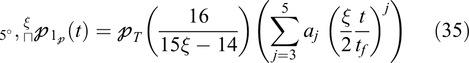
where a_j is shown in Table 5.

Trajectory generation

The duration of the first and second transient stages comprises points of the path belonging to different geometric curves. In this manner, the entire path is divided into five parts: (a) the first one corresponds to the first quarter of the circle during the first transient stage, (b) the second one concerns points on the straight line during the first transient stage, (c) the third one involves points on the straight line during the stationary stage, (d) the fourth one implies points on the straight line during the second transient stage, and (e) the fifth one corresponds to the points on the second quarter of the circle during the second transient stage (see Figure 15).

Figure 15.

Path divisions in terms of the transient and stationary stages.

Equations (38) to (47) present the coordinates at which the foot is positioned, according to the division given in Figure 15.

First quarter of the circle in the first part of the transient is

$x\left(t\right)=r C{\sigma }_1\left(t\right)+d_2$

38

$y\left(t\right)=r S {\sigma }_1\left(t\right)-h$

39

Straight line in the first part of the transient is

$x\left(t\right)=\frac{{\mathcal{p}}_T}{2}-5°,{}_{\sqcap }{}^{\xi }\mathcal{p}{}_{1_{\mathcal{p}}}\left(t\right)$

40

$y\left(t\right)=-h+r$

41

Straight line in the stationary stage is

$x\left(t\right)=\frac{{\mathcal{p}}_T}{2}-5°,{}_{\sqcap }{}^{\xi }\mathcal{p}{}_{2_{\mathcal{p}}}\left(t\right)$

42

$y\left(t\right)=-h+r$

43

Straight line in the second part of the transient is

$x\left(t\right)=\frac{{\mathcal{p}}_T}{2}-5°,{}_{\sqcap }{}^{\xi }\mathcal{p}{}_{3_{\mathcal{p}}}\left(t\right)$

44

$y\left(t\right)=-h+r$

45

Second quarter of the circle in the second part of the transient is

$x\left(t\right)=-r S{\sigma }_2\left(t\right)-d_2$

46

$y\left(t\right)=r C{\sigma }_2\left(t\right)-h$

47

where

${\sigma }_1\left(t\right)=\frac{5°,{}_{\sqcap }{}^{\xi }\mathcal{p}{}_{1_{\mathcal{p}}}\left(t\right)}{r}$

48

${\sigma }_2\left(t\right)=\frac{5°,{}_{\sqcap }{}^{\xi }\mathcal{p}{}_{3_{\mathcal{p}}}\left(t\right)-67.708cm}{r}$

49

In order to obtain the joint variables, L_AB, L_BC, and θ, in terms of time, the coordinates given by equations (38) to (47) are substituted in equations (31), (32), and (34), correspondingly. When t changes from 0 s to t_f, we have joint variable evolution.

Results

The graphics shown in Figures 16 and 17 express the temporal history of the task, whereas Figures 18 and 19 show the joint coordinates.

Figure 16.

Evolution of coordinates referred to ${\widehat{x}}_F$ with respect to time.

Figure 17.

Evolution of coordinates referred to ${\widehat{y}}_F$ with respect to time.

Figure 18.

Variable length for elements formed between AB and BC.

Figure 19.

Angular variation of the actuator at point B, θ.

On the one hand, Figure 16 deals with coordinates referred to ${\widehat{x}}_F$ . This evolution in relation to time was obtained through the use of equations (38), (40), (42), (44), and (46).

On the other hand, the graphics in Figure 17 present the evolution in relation to time of the coordinates dealing with ${\widehat{y}}_F$ . It was obtained when time in equations (39), (41), (43), (45), and (47) varies from 0 s to t_f.

Regarding joint space, the graphics in Figures 18 and 19 deal with $L_{AB}=L_{BC}$ and θ, respectively. In Figure 18, the lengths of L_AB and L_BC increase when the foot moves upward, as time changes from 0 s to 0.57 s, and they decrease, from 1.43 s to 2 s, when the foot descends.

Figure 19 shows the evolution of θ through time during the walking gait. Note the angular variation of link BC with respect to link AB in Figure 20, which presents four postures of the left PL-based leg.

Figure 20.

Four postures of the PL-based leg corresponding to different instants of time, where (a) 0.25 s, (b) 0.7 s, (c) 1.2 s, and (d) 1.72 s. PL: Peaucellier–Lipkin.

With respect to the right robotic leg, the evolution of the horizontal coordinate is shown in Figure 21, whereas Figures 22 and 23 present the evolution of joint variables. Due to the fact that the hip travels at a constant height, and its path is parallel to the floor, and the foot is in contact with the terrain, the linear actuators, concerning L_AB and L_BC, stay motionless (Figures 22 and 24). The only actuator in motion is the revolute one (Figure 23).

Figure 21.

Evolution of coordinates referred to ${\widehat{x}}_F$ with respect to time in the right robotic leg.

Figure 22.

Constant length of linkages AB and BC concerning the right robotic leg.

Figure 23.

Angular variation of the actuator at point B in the right robotic leg, θ.

Figure 24.

Dynamic sequence of four postures of right PL-based legs, where (a) 0.25 s, (b) 0.7 s, (c) 1.2 s, and (d) 1.72 s. PL: Peaucellier–Lipkin.

Figure 24 shows a dynamics sequence of four postures of the right leg, whereas Figure 25 shows a dynamic sequence of four postures of both PL-based legs.

Figure 25.

Dynamic sequence of four postures of both PL-based legs, where (a) 0.25 s, (b) 0.7 s, (c) 1.2 s, and (d) 1.72 s. PL: Peaucellier–Lipkin.

Second simulation

Conditions

In this second simulation, we reproduce an actual human gait. In Figure 26, we show a set of six pictures illustrating a dynamic animation sequence, considering the right leg movement of a person. It shows the path followed by the ankle. As can be seen in Figures 2 and 7, point A coincides with the human ankle, thus the path presented in Figure 26 is the one to be reproduced by point A of the exoskeleton. This path is confirmed by O’Connor et al. ³²

Figure 26.

Path generated by a person’s right leg and ankle.

Trajectory conditions

Table 6 presents the trajectory conditions, which involve the maximum horizontal stroke, maximum vertical stroke, and the time elapsed in the complete flight phase.

Table 6.

Maximum strokes and duration of the flight phase concerning the path generated by the human right leg and ankle shown in Figure 21.

Description	Value
Maximum horizontal stroke	92.7 cm
Maximum vertical stroke	11.16 cm
Duration (tf)	1.7 s

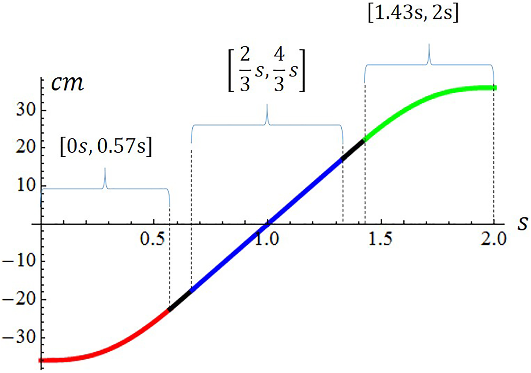
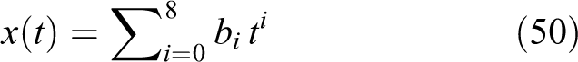
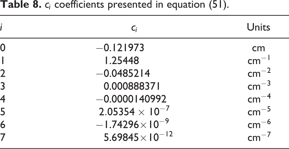
The trajectory generated by the human ankle is adjusted by means of equations (50) and (51), where coefficients b_i and c_i are presented in Tables 7 and 8

$x\left(t\right)={\displaystyle {\sum }_{i=0}^8{b}_i{t}^i}$

50

$y\left(t\right)={\displaystyle {\sum }_{i=0}^7{c}_i{x}^i\left(t\right)}$

51

Table 7.

b_i coefficients in equation (50).

i	bi	Units
0	1.92497	cm
1	−123.463	${\text{cm s}}^{-1}$
2	1379.41	${\text{cm s}}^{-2}$
3	−5772.72	${\text{cm s}}^{-3}$
4	11387.7	${\text{cm s}}^{-4}$
5	−11467.7	${\text{cm s}}^{-5}$
6	6154.24	${\text{cm s}}^{-6}$
7	−1681.99	${\text{cm s}}^{-7}$
8	184.314	${\text{cm s}}^{-8}$

Table 8.

c_i coefficients presented in equation (51).

i	ci	Units
0	−0.121973	cm
1	1.25448	${\text{cm}}^{-1}$
2	−0.0485214	${\text{cm}}^{-2}$
3	0.000888371	${\text{cm}}^{-3}$
4	−0.0000140992	${\text{cm}}^{-4}$
5	$2.05354\times {10}^{-7}$	${\text{cm}}^{-5}$
6	−1.74296 $\times {10}^{-9}$	${\text{cm}}^{-6}$
7	5.69845 $\times {10}^{-12}$	${\text{cm}}^{-7}$

Results

Figure 27 presents the evolution of the horizontal and vertical travel concerning the ankle of the right PL-based leg, and Figures 28 and 29 show the temporal history of the joint variables.

Figure 27.

Horizontal and vertical range of the right ankle during a human gait.

Figure 28.

Evolutions of the variable lengths concerning the joints between points A and B and between points B and C.

Figure 29.

Evolution of the θ variable.

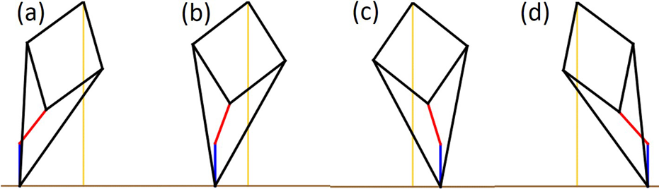
Finally, in Figure 30, we present six postures dealing with the dynamic animation sequence of the right PL-based leg.

Figure 30.

Path reproduced by point A of the PL-based exoskeleton, where (a) 0.1 s, (b) 0.2 s, (c) 0.4 s, (d) 0.6 s, (e) 0.9 s, and (f) 1.1 s. PL: Peaucellier–Lipkin.

Discussions

In the previous simulations, we observe certain attributes that allow clear differentiations with respect to other exoskeletons.

They highlight the fact that the support legs, in both simulations, use only one of their DOFs to perform its task. This is an important advantage in consideration of the control system. Traditional systems require two DOFs to perform the same task. In this way, the control of only one actuator per leg is much simpler than the control of two of them. This advantage is also observed when the ankle of the robotic leg traces the straight line between the two quarters of circles presented in Figures 11, 15, and 20.

When the left leg, in the first simulation, executes the transfer phase, it makes use of its three actuators when it traces the initial and final quarters of the circles; nevertheless, the two linear actuators provide the same displacement in a dependent manner. When one of them increases or decreases its stroke, the other one also does it in the same magnitude. Thus, they become a single DOF, which acts coordinately with the revolute one, concluding that the robotic leg is a two-DOF positioning device. It means that the controller controls the rotary actuator and the equal displacements of both linear motors. According to this argument, we ask the next question: What is the reason in using two linear actuators acting dependently instead of one? It is important to remember that linkages AB and BC have to change their lengths, but there is a revolute joint between them, placed at point B, obstructing the installation of a mechanism capable of modifying both linkage lengths at the same time and at the same rate of motion. Several solutions were proposed, for example, the use of a two-DOF telescopic mechanism, formed by a revolute joint and a prismatic one, installed between points A and C; it seemed to be promising, but the ability to trace exact paths, with the use of a PL mechanism, obliges to conserve the basic mechanical structure, which makes use of only one DOF (the revolute joint installed at B) instead of the two DOFs concerning the telescopic mechanism. Thus, the solution of two linear motors, acting dependently, seems to be the simplest one.

Although the nonanthropomorphic exoskeleton concerning this research uses its three actuators per leg in the mode of two-DOF, because the two linear motors are confined to move dependently, it is possible to move them independently. This attribute provides redundant legs in terms of the conditions of the task. Typically, a robotic leg should have the same number of DOFs for positioning. More than this number is referred to as kinematically redundant leg. ⁴¹ Nevertheless, the extra DOFs found in redundant positioning devices are conveniently exploited to meet a number of additional constraints on the solution of the inverse kinematics, ⁴² to generate an internal joint motion that reconfigures the structure according to given task specifications, ⁴³ and to obtain a more versatile positioning device in terms of its kinematical configuration and its interaction with the environment. ⁴⁴ Thus, redundancy is a source of freedom in task execution, because it provides the robot mechanism with an increased level of dexterity. ⁴⁵ According to this attribute, consider the circular path, traced by the nonanthropomorphic leg presented in Figure 31. Due to the fact that this leg is based on the one-DOF PL mechanism, it easily traces the path with the use of only one DOF, the revolute one. But the mechanism has to be previously configured to provide concave or convex circular paths, according to cases 2 and 3, presented in Figure 8. In front of traditional anthropomorphic exoskeletons, which use two DOFs per leg when they trace circular arcs, it represents an advantage in terms of control (In terms of the user, it could be used for the initial stages of its conditioning training for rehabilitation, allowing a gradual adaptation in the use of the exoskeleton through simple trajectories.

In Figure 31 we show how a PL-based leg performs a circular arc during a transfer phase. Prior to the execution of this task, the robotic leg had to undergo a configuration by means of its two linear actuators; linkage BC must be shorter than linkage AB, according to case 3. The radius of the arc depends on the location of the center of rotation, which is obtained by the correct ratio between the lengths AB and BC. In this manner actuators AB and BC act independently, nevertheless this 2-DOF configuration occurs before the 1-DOF gait, they are decoupled. Once the configuration is achieved, actuators AB and BC remain motionless during the gait.

As it shown in the second simulation, this nonanthropomorphic exoskeleton is able to reproduce common anthropomorphic gaits by the aid of their three motors per leg. As it has been discussed, the displacements of the linear actuators are considered dependent, so the number of DOFs of the joint space coincides with the number of DOFs of the task.

Most anthropomorphic exoskeletons need to have their legs firmly fixed to the user’s legs with their joints precisely coincident, which is a difficult task to achieve. In the case concerning the nonanthropomorphic PL-based exoskeleton, the robotic and human legs are not restricted to coincide precisely. The user is supported by a harness and the tips of her or his toes are fixed to the robotic ones. Furthermore, the human heels and ankles are free to move, providing to the user’s foot certain freedom of rotation; therefore the robotic ankle does not necessarily coincide with the user’s ankle. With respect to the knees, the exoskeleton does not have ones, and then it is not necessary to restrict the motion of the user’s knee.

In consideration of the ability to perform cases 1, 4, and 5, shown in Figure 9, the PL-based exoskeleton is capable of adjusting its size according to the user’s size; this is an advantageous skill in front of other exoskeletons, which are specifically designed according to the user's physical conditions.

The PL-based exoskeleton is a bulky wearable robot. This attribute seems to be nonadvantageous, in front of others. Nevertheless its mechanical architecture has several bars, resulting in a stiff and strong structure with the ability of distributing forces and moments of forces better than traditional exoskeletons. According to this attribute and a particular design, this exoskeleton can be used as the basis of legged forklifts.

Anthropomorphic exoskeletons allow the user to sit down or reach low postures. This nonanthropomorphic exoskeleton is not capable of performing such tasks.

Figure 31.

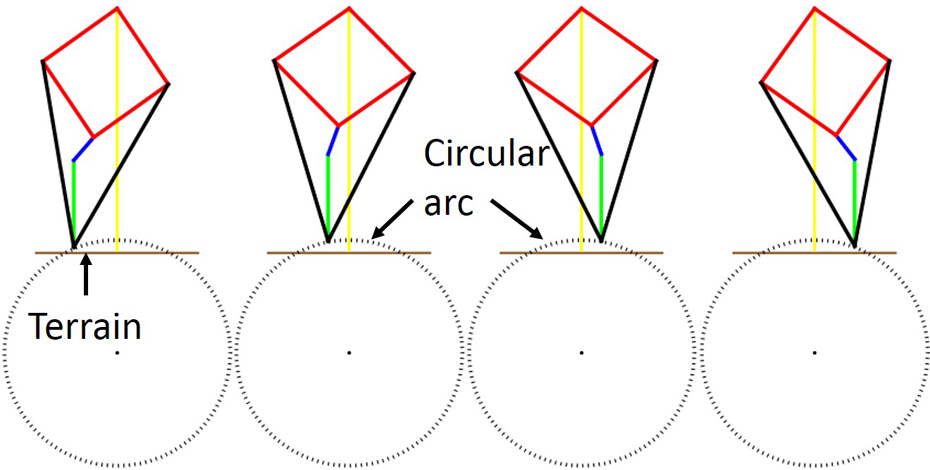
Circular path reproduced by a point using only one DOF after configuration. DOF: degree of freedom.

Conclusions

A new mechanical architecture of exoskeletons, intended for assistance and rehabilitation, is proposed. It is arranged in a nonanthropomorphic way, but is capable of providing complex trajectories, including the one related to actual anthropomorphic gait. Due to the nature of the one-DOF PL mechanism, which is the basis of this exoskeleton, linear translation, resulting from the rotation of the input link, is easily provided. This advantage was considered the strongest attribute in the conceptualization of the novel exoskeleton for lower limbs described herein. When the exoskeleton has a leg in the support phase, on flat and horizontal ground, the leg uses only one DOF, associated with the active revolute joint. The use of the second and third DOFs is considered when the robotic foot ascends or descends, during the transfer phase. Compared with other anthropomorphically arranged exoskeletons, an advantage of this nonanthropomorphic wearable robot is that the joints of the robot and those of the user need not match with precision. The user is mounted on the exoskeleton by means of a harness and his/her feet are fixed to the robotic end effectors. The user’s knees do not match any specific robotic joint, because the wearable robot does not have knees.

To be used as a leg of a nonanthropomorphic wearable robot, the basic PL mechanism has undergone major changes: (a) the addition of two more DOFs, which enhance mobility and are responsible for the ability to trace complex paths, and (b) the inclusion of the OSS, which is responsible for keeping an unalterable description of the orientation between the robotic foot and the pelvic link. The challenge was to find the way to introduce three actuators, two prismatic joints, and the OSS that is composed of four timing belts and eight toothed pulleys, among a tangle of links that cross certain joint axes during their movement, while at the same time maintaining a light and stiff structure, capable of supporting both its own weight and the payload. Despite this entanglement of links, the presence of eight bars allows good distribution of the total load across the entire strong structure. Thus, considering its suitable stiffness, along with the corresponding mechanical adjustments, and based on a pertinent mechanical design, the architecture of this exoskeleton could be used as a legged forklift.