
Abstract
This article deals with the kinematics and dynamics of a novel leg based on the Peaucellier–Lipkin mechanism, which is better known as the straight path tracer. The basic Peaucellier–Lipkin linkage with 1 degree of freedom was transformed into a more skillful mechanism, through the addition of 4 more degrees of freedom. The resulting 5-degree-of-freedom leg enables the walking machine to move along paths that are straight lines and/or concave or convex curves. Three degrees of freedom transform the leg in relation to a reachable center of rotation that the machine walks around. Once the leg is transformed, the remaining 2 degrees of freedom position the foot at a desirable Cartesian point during the transfer or support phase. We analyzed the direct and inverse kinematics developed for the leg when the foot describes a straight line and found some interesting relationships among the motion parameters. The dynamic model equations of motion for the leg were derived from the Lagrangian dynamic formulation to calculate the required torques during a particular transfer phase.
Keywords
Introduction
In 1864, Charles Nicolas Peaucellier, a French army officer, developed a very special mechanism by joining eight links to convert circular motion into exact linear motion. Independently, the Russian mathematician Lipman Lipkin1–4 developed the same linkage, explaining it in more detail, and so the mechanism is named the Peaucellier–Lipkin (PL) linkage. Additionally to the ability to trace linear paths, Shigley and Uicker 5 say that the PL mechanism can be made to trace a true circular arc of very large radius.
The PL mechanism has been studied in different positions and configurations, 6 as well as in its distinct inversions. 7 Other researchers have carried out systematic inquiries dealing with optimum dimensional synthesis. 8 Examples of applications of the PL mechanism are a phonograph pickup arm, 9 the suspension for electric wheels, 10 and two walking machines: one with the ability to move four skis to walk 11 and the other that uses six legs to walk. The legs of the latter are fixed to a circular chassis. 12 These two machines only have the capacity to move in a straight line path, making their adaptation to changing roads impossible. Nevertheless, most of the applications in the above-mentioned studies consider just the basic PL mechanism with no additional degrees of freedom (DOFs). There is also a remarkable lack of information concerning the use of the PL mechanism as a robotic leg or propulsion unit, motivating us to develop a leg that can describe lines and arcs with different centers of rotation.
Table 1 shows the comparative list of the skills in different mechanical architectures that use the PL mechanism and the Novel Propulsion Unit (NPU) presented in this article.
Comparative list of skills.
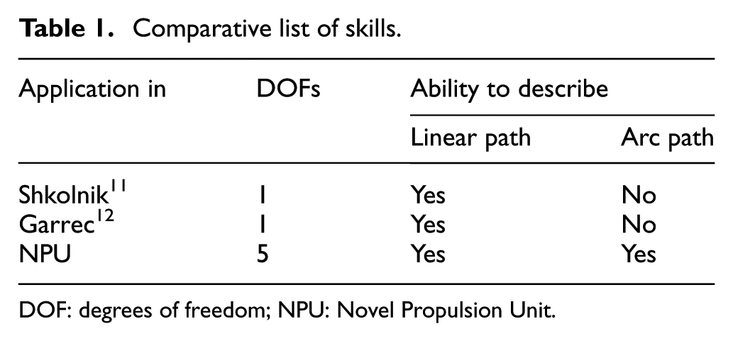
DOF: degrees of freedom; NPU: Novel Propulsion Unit.
The study of walking machines has increased over the last decades, resulting in the development of new propulsion mechanisms, along with more detailed kinematic and dynamic studies. For example, Roy and Pratihar13–16 developed studies on the kinematics and dynamics for a six-legged robot, applying the Lagrangian dynamic formulation and Wang et al. 17 studied the full body kinematics of a radial symmetrical six-legged robot and calculated its kinetic energy by means of a dynamic model using the Lagrangian method.
This work develops the kinematics and dynamics for a novel robotic leg based on the PL mechanism. This leg has 5 DOFs, but only 2 of them are used in the support and transfer phases. The other 3 DOFs are used exclusively when the foot needs a reconfiguration to describe a different path during the transfer phase. 18 Our work focuses only on the transfer phase when joint F traces a linear path.
Description of the hexapod robot
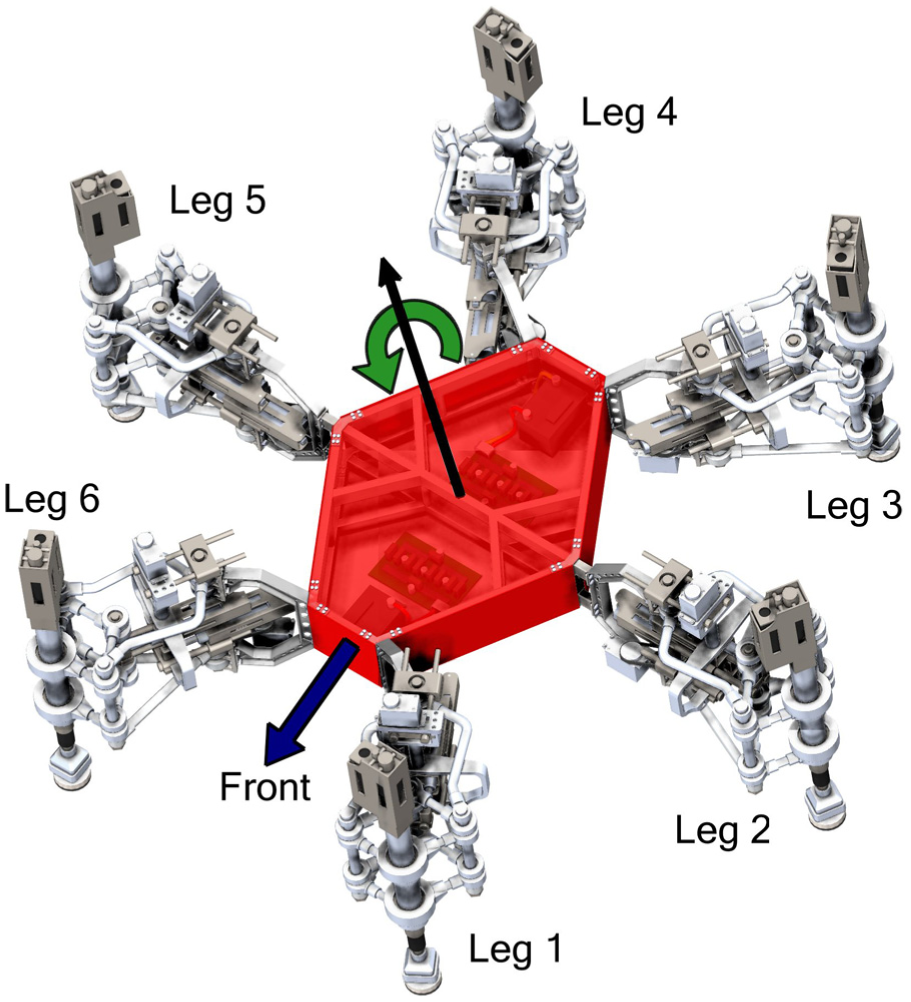
Figure 1 shows the computer-aided design (CAD) model of the six-legged robot using the propulsion unit studied in this work. It consists of a body that is an irregular hexagonal trunk and six legs. Each leg is composed of eight links driven by five actuators. Two of the actuators are rotative and three are linear, as shown in Figure 2.
CAD model of the six-legged robot.

Actuators in the robotic leg.
The kinematics and dynamics modeling in this work describes just one leg in a transfer phase, because the movement of the other legs is similar. The kinematics parameters are calculated by direct and inverse kinematics to describe the motion of the leg and to find the necessary torque in rotary actuator B. The aim of this research is to derive the kinematic equations of all the links of the leg so that the required joint velocities and accelerations necessary for the dynamic equations to establish the joint torques can be determined.
Kinematics of the propulsion unit
To develop the kinematic leg description, it is assumed that joint A is fixed and that the linear velocity of the foot depends on the dynamic characteristics of rotary actuator B. The height of the foot is constant during the transfer phase. The kinematic study has been divided into three sections: mechanism description, direct kinematics, and inverse kinematics.
Mechanism description
The propulsion unit, which is based on the PL linkage, was modified by adding 4 DOFs, resulting in a new Reconfigurable Propulsion Unit.
18
This mechanism has six rotational joints called A, B, C, D, E, and F, and the eight links are as follows: AB, AD, AE, BC, CD, CE, DF, and EF. Their lengths are

Description of the robotic leg joints.
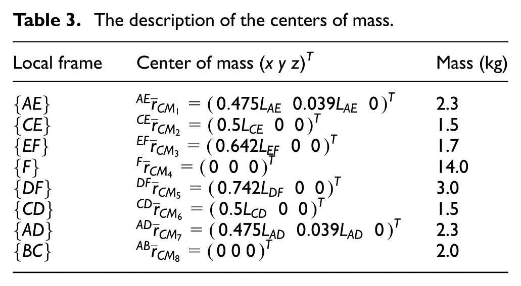
Table 2 shows the lengths of the eight links. Figure 5 is the sketch of the leg including the position of the centers of mass, which are calculated using a CAD program in a local link frame as described in Table 3. The variables used to describe the centers of mass are specified in section “Direct kinematics.” The center of mass of link BC is coincident with joint B, due to the geometry of the real link, which includes the motor mass. Link AB is considered the fixed link. The translation axis of link F (which includes the linear actuator F and the foot (Figures 2 and 3)) and the rotation axis of joint F are collinear. Finally, the center of mass of this last link is coincident with the origin of the frame
Length of links.

The description of the centers of mass.
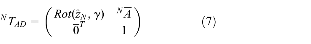
The required frames that describe the position of the centers of mass for the links are approached in the matrix of translation described in equations (1)–(8)
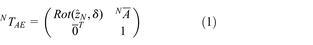
where


where

Description of the joints for the robotic leg.
Direct kinematics
To describe the kinematics of the leg, it is necessary to find the positions, angular velocities, and angular accelerations of the links as functions of θ, considering the lengths
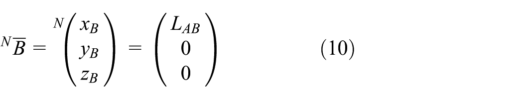
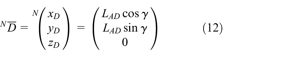
The positions of joints A, B, C, D, E, and F and the characteristic angles are described in equations (9)–(24), according to the sketch shown in Figure 4. Joint A, described by

Joints B, C, D, E and F, defined by


where


The relative angles


Kinematic and dynamic analysis requires the absolute angles measured in the frame {N}, which is why the absolute angular positions


The angular velocities of the links are calculated as the derivative of the angular positions with respect to time (t). For example, the angular velocity

and the other angular velocities for the links are similarly calculated.
The angular accelerations for the links are calculated as derivatives of the angular velocities with respect to time (t). For example,

and a similar process is applied to obtain the other accelerations.
To calculate the linear velocities of the links in the centers of mass, it is necessary to describe the center of mass positions from


Due to the symmetry of the mechanism, it is expected that the angular displacement utilized to describe links AD, AE, CD, CE, DF, and EF would be dependent on position, velocity, and angular acceleration.
Inverse kinematics
This section describes how

The lengths of links


Finally, using equation (43), the value of

Trajectory generation
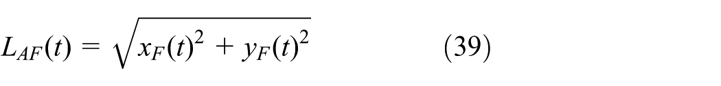
The main purpose of the foot trajectory is to determine the required joint variable


where
The index
Dynamics of the propulsion unit
Due to the simplicity of the mechanism, the leg motion equations are derived by applying the typical Lagrangian dynamic formulation for mechanical systems, 20 but the results are similar to those using formulations employed by Hollerbach 21 or Kane 22 that are normally used in robotic mechanical systems. In the dynamic analysis, the mass of each link is considered to be concentrated at the point called the center of mass, described in Table 3 and shown in Figure 5. The mass moment of inertia is calculated at the center of mass of each link, with respect to its local frame. It is calculated using a CAD model and the values are shown in Table 4.

Description of center of mass and joints.
Mass moment of inertia for the links.

To obtain the dynamic model, the following considerations are assumed:
Friction in the joints is negligible due to the use of bearings.
The links of the mechanism move on the plane formed by
The densities of the links are constant.
Development of the dynamic equations
The dynamic analysis of the leg is developed for the transfer phase, in which the forces of the ground reaction to the foot are equal to zero. This is because there is no terrain interaction and the positions of the mass of the mechanism’s links are constant on the vertical plane.
The dynamics of the mechanism are calculated using the general Lagrangian equation of motion (47) where

Due to the kinetic or potential energy of the system, which is the sum of the kinetic or potential energy of each link, it is possible to use the derivative sum rule 23 to independently apply equation (47) for each link and obtain the torque required by each link, as in equation (49)

where

where
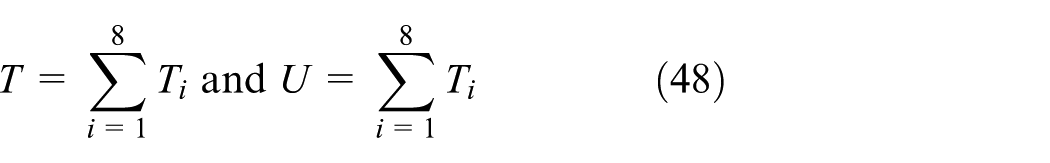
Finally, to determine the total torque required to move the leg by joint B, it is necessary to add all the torques according to
Results and discussion
The physical parameters employed in the simulation are described in Tables 2–4. The positions of the links and their centers of mass when the foot follows a linear path using a polynomial profile can be seen in Figure 6. The time used to follow this trajectory (equation (44)) is

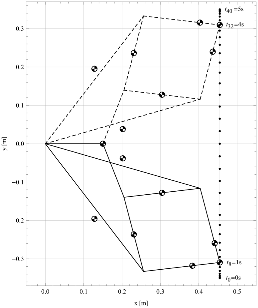
Position of the leg describing a linear path when
Figure 6 shows the two positions of the leg when
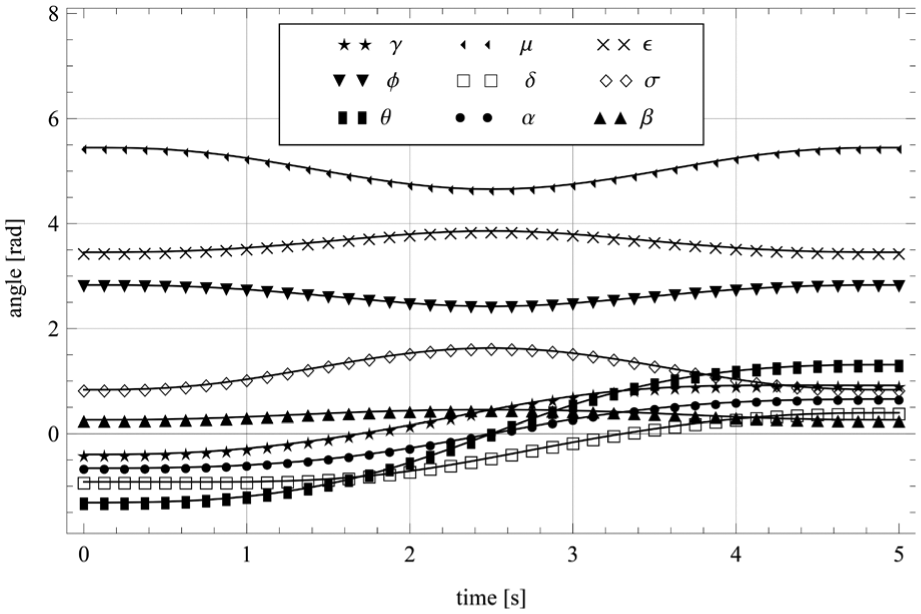
Figure 7 shows the angular positions of the links varying as a function of time, using equations (15)–(28). It is interesting to observe equation (52), because it expresses a complementary relationship between the relative angles σ and µ (links DF and EF), and the relative angles φ and ∈ (links CD and CE). In addition, equation (53) expresses a supplementary relationship between the absolute angles


Angular position of the links.
Those relationships are due to the symmetry of the mechanism, which is consistent with the description given in section “Direct kinematics.” The relations expressed in equation (53) indicate that links CE and DF, as well as CD and EF, are always parallel.
The angular velocities were calculated using the process described in equation (29) and the results are shown in Figures 8 and 9. Due to the fact that the velocity is the variation with the time of the position, if the change of position is the same in some angles, consequently it is possible to generate relationships between the angular velocities. The relationships of the relative and absolute velocities presented in equations (55) and (56), respectively, are confirmed if equations (52) and (53) are derived with respect to time. Finally, the third relation is a vertical reflection relationship between the angular velocities


Angular velocities of the links.
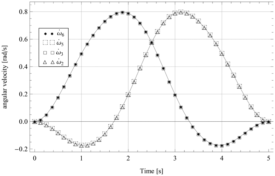
Absolute angular velocity in the rhombus formed by links CD, DF, EF, and CE.
Figure 10 shows the angular acceleration of the leg links calculated according to the process described by equation (30). Because the acceleration is the variation with the time of the velocity, consequently it is possible to generate interesting relationships between the angular accelerations. The relationships of the relative and absolute accelerations are presented in equations (58) and (59), respectively, and are confirmed if equations (55) and (56) are derived with respect to time. At least a double reflection relationship in time between the angular acceleration


Angular acceleration of the links.
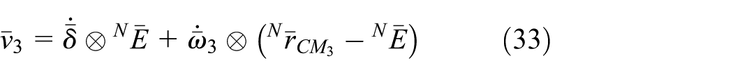
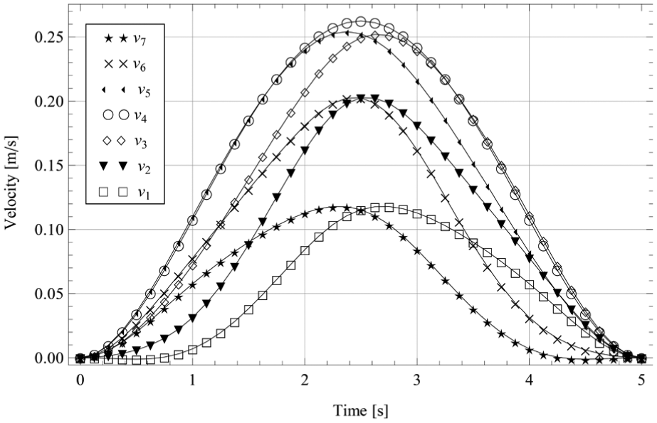
The linear velocity of each link was calculated at its center of mass, shown in Figure 11. The equations used to calculate the velocity for the foot are described in equations (31)–(38).
Linear velocity of the links.
According to the leg configuration, the center of mass located in the foot is the furthest from the inertial frame
The previously described parameters are necessary for the dynamic model so that the torque can be calculated and the leg moved. According to these parameters, it is possible to estimate the link that will require more torque, assuming the mass as the more important parameter, but also considering position, velocity, and acceleration. It is postulated that the foot requires more torque because it has the biggest mass. Another important link to consider is the DF link, due to its mass, velocity, and acceleration.
Torque is calculated independently for each link using equation (35). The values of the required torque for the links, with the exception of the foot, are illustrated in Figure 12. It shows that link DF

Torque required by the links.
Figure 13 shows the torque that is required for moving the foot
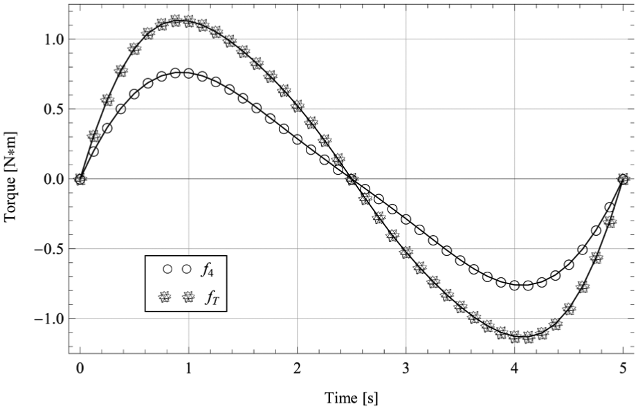
Foot torque and total torque in the leg.
Conclusion
Our article describes the kinematics and dynamics for a novel robotic leg based on the PL mechanism when the foot follows a linear path on a transfer phase.
Interesting relationships in the positions, velocities, and angular accelerations (complementary, supplementary, reflective, and double reflective) between the mechanism links were found that are useful for decreasing the number of kinematic equations and thus reducing the quantity of calculations.
The use of the Lagrangian equations of motion for the mass of each link of the mechanism enabled the quantification of the required torque for each link, and the proposal of improvements in mechanism design, such as the reduction of mass in the foot.
Most robotic legs are based on open or serial kinematic chains. Due to the fact that the PL robotic leg is based on a parallel linkage with eight bars, it distributes forces and torques in a manner superior to that of the open or serial kinematic chains. Given that the robotic leg is based on the PL mechanism, which traces exact paths as linear or circular curves, it requires the employment of only two actuators to position the foot. These are the main advantages to using the apparently complex PL robotic leg, compared with other mechanical leg architectures.
Footnotes
Academic Editor: Yangmin Li
Declaration of conflicting interests
The author(s) declared no potential conflicts of interest with respect to the research, authorship, and/or publication of this article.
Funding
The author(s) disclosed receipt of the following financial support for the research, authorship, and/or publication of this article: The authors acknowledge to Consejo Nacional de Ciencia y Tecnología (CONACyT) for the scholarship support.