Trend-aware motion planning for wheeled mobile robots operating in dynamic environments

Abstract

Planning collision-free trajectories is essential for wheeled mobile robots operating in dynamic environments safely and efficiently. Most current trajectory generation methods focus on achieving optimal trajectories in static maps and considering dynamic obstacles as static depending on the precise motion estimation of the obstacles. However, in realistic applications, dealing with dynamic obstacles that have low reliable motion estimation is a common situation. Furthermore, inaccurate motion estimation leads to poor quality of motion prediction. To generate safe and smooth trajectories in such a dynamic environment, we propose a motion planning algorithm called trend-aware motion planning (TAMP) for dynamic obstacle avoidance, which combines with timed-elastic band. Instead of considering dynamic obstacles as static, our planning approach predicts the moving trends of the obstacles based on the given estimation. Subsequently, the approach generates a trajectory away from dynamic obstacles, meanwhile, avoiding the moving trends of the obstacles. To cope with multiple constraints, an optimization approach is adopted to refine the generated trajectory and minimize the cost. A comparison of our approach against other state-of-the-art methods is conducted. Results show that trajectories generated by TAMP are robust to handle the poor quality of obstacles’ motion prediction and have better efficiency and performance.

Introduction

The generation of safe and feasible trajectories for wheeled mobile robots is essential to accomplish the autonomous navigation in confined and dynamic environments ^1,2 without human intervention. In recent decades, reliable motion planning approaches for the mobile robots which operate with neither an onboard human presence nor transmitted control has been spotlighted in plenty of cruise and transportation services.

Many existing motion planning approaches ^{3 –7} have focused on generating the optimal trajectories online instead of conventional paths ⁸ to deal with increasingly complex practical applications. It is common that mobile robots are deployed under partial-known environments that have the presence of random dynamic obstacles (e.g. pedestrians and other social vehicles) and static objects in most realistic application scenarios. Under this circumstance, the majority of existing path planners ^{9 –11} fail to search a collision-free path for mobile robots, due to the conflict caused by moving obstacles. On the contrary, a general motion planner, ^12,13 which incorporates temporal and kinodynamic constraints, ^{14, 15} has more success rate in spite of optimality and real-time capability. This is mainly because the obstacles’ future proxemic behavior is revealed by adding the time dimension. To execute the planning algorithm in real time and achieve a relatively optimal result simultaneously, the relevant approaches ^16,17 usually modify a path pruned from the global path to reduce the computing effort. Meanwhile, they consider trajectory time consumption, kinodynamic, clearance from obstacles, and compliance with the desired path as the constraints in the trajectory optimization.

However, avoiding stochastic moving obstacles is still a tough challenge for the motion planner even all the objectives are optimized sufficiently. Especially when mobile robots encounter a random crossing situation, in spite of having ideal robotic self-localization, ^18,19 a general motion planner ²⁰ cannot guarantee to generate a collision-free trajectory. There are two main reasons accounting for the poor planning solution: (1) it is still difficult to acquire precise velocity and acceleration of an unknown object efficiently even with advanced sensors and algorithms at present ²¹ and (2) most local motion planners only pay close attention to a obstacle’s current state instead of the whole obstacle dynamics. For the former case, the actual measurement contains errors and noise inevitably, which leads to the situation that most local motion planners are unable to maintain long-term optimality and can only deal with imminent crossing obstacles using a replanning mechanism. ^22,23 As to the latter case, alternatively, the moving trends of obstacles are neglected conventionally, which is a piece of vital information for local motion planners to avoid the obstruction or even collisions caused by dynamic obstacles.

As to solve the problems above, we introduce a new dynamic obstacle avoidance approach called trend-aware motion planning (TAMP) that is capable of generating collision-free trajectories. TAMP is built by the combination of the work of Rösmann et al. ¹³ and our proposed technique called trend-aware trajectory deformation (TATD) which deforms a given trajectory into a collision-free trajectory for dynamic obstacle avoidance. Due to the inaccurate motion estimation of dynamic obstacles, we hypothesize that crossing obstacles are goal-driven, which indicates the moving direction of the crossing obstacles only varies in an appropriate interval. TAMP takes advantage of dynamic obstacles’ motion prediction based on their inaccurate motion estimation to predict their moving trends. By analyzing the limitation of the mobile robot’s and dynamic obstacles’ moving trends, we formulate the dynamic obstacles avoidance problem into an optimization problem. Furthermore, the optimization problem also has the constraints of kinematics, dynamics, and time consumption. To solve the problem, the multi-objective optimization problem is transformed into an approximative nonlinear squared optimization problem. The objective of TATD is local as it only rests upon a few adjacent configurations, which result in a sparse structure, thus ensuring optimality and efficiency. An iterative mechanism is implemented owing to the computational advantage. Hence, the planned trajectory vertices can be deformed in time with respect to safety and optimality in case of a sudden change or even reverse in the direction of obstacles’ movement. TAMP makes the service concept inherent to social mobile robots’ motion planning, and it chooses a socially compliant way ahead of a minimum time way, which complies with the social norm. But TAMP still endeavors to minimize the time consumption under this condition. Therefore, as is shown in Figure 1, when the encounter occurs, the mobile robots implemented with TAMP take the detour and bypass behind obstacles’ moving direction while maintaining a safe separation from obstacles rather than getting in the way of the obstacles or stuck in place due to the misleading of the disturbed motion prediction.

Figure 1.

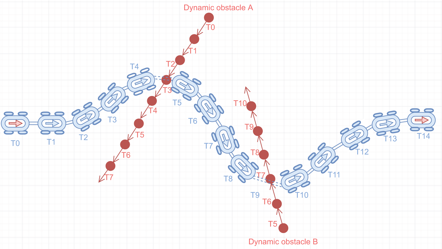
A single-trajectory generation using trend-aware motion planning. T represents for time stamp. The robot states in T0 and T14 represent start and goal, respectively. T4 and T8 are the crucial moment in which TATD dynamically deforms the trajectory away from the moving obstacles with respect to the trends of the obstacles. TATD: trend-aware trajectory deformation.

To show the advantage of our approach experimentally, we have compared TAMP’s performance against the timed elastic bands (TEBs) planner ¹³ and TEB equipped with homology class (HC) ²⁴ exploration. Averagely, our results indicate that TAMP continuously generates more feasible trajectories than the state-of-the-art TEB and TEB + HC planners, which results in lower path length cost, lower time consumption, and higher stability.

The remainder of this article is structured as follows. In the second section, we review the related work. Then we describe TAMP in the third section. The fourth section shows the experiments and results. Finally, we conclude this article in the final section.

Related work

In this section, we describe the approaches relevant to the collision-free path or trajectory generation for dynamic obstacle avoidance. Modeling dynamic obstacles as static obstacles in a short replanning period is a common way adopted by many approaches. Devin Connell and Hung Manh La² use the RRT* ²² algorithm as well as Sven Koenig and Maxim Likhachev ²³ implement the dynamic A* algorithm for replanning in a dynamic environment with random, unpredictable moving obstacles. Although the generated paths are approximate optimal within the limits, the risk of colliding with the dynamic obstacles is still existing without incorporating the time dimension. When the replanning time expires, the approaches will fail to give the path in time. On the contrary, our planner takes the time interval of adjacent configurations into account for avoiding collision cautiously.

Velocity obstacles ²⁵ are used to compute appropriate velocities to avoid collisions with dynamic obstacles. Dynamic window approach ²⁶ searches the optimal control speed of the robot corresponding to the optimal trajectory in the velocity space to avoid local obstacles. Both the approaches deal with dynamic obstacles with a time interval, however, they can run into local minima easily and get stuck without other solutions. TAMP, on the other hand, implements a planning process with an appropriate time horizon. Thus, it has sufficient space and time intervals to optimize near-term objective functions for generating safer and more socially compliant trajectories.

Phillips and Likhachev ²⁷ and Narayanan et al. ²⁸ describe a safe interval technique that gives a robot the ability to safely navigate in the dynamic environment with the presence of moving obstacles. However, the technique assumes that the future trajectories of dynamic obstacles are predicted accurately, which is difficult to maintain in actual applications. Generally speaking, the moving obstacles’ motion is probabilistic so that it can only be approximated in a local interval. TAMP, on the other hand, is prepared for the situation that it only demands the current velocity and position of the obstacles instead of the whole accurate future trajectory, and simple estimation of the trajectory implemented over a local time horizon is sufficient for the planner to avoid the collision.

Park et al. ⁷ describe a dynamic obstacle modeling technique that computes a conservative bound on the position of the moving obstacles based on the predicted motion and then avoids collisions by solving an optimization problem. Instead of only modeling the future position of dynamic obstacles, TAMP attaches importance to the moving trends of obstacles.

The methodology of trend-aware motion planning

Trend-aware motion planning is composed of TATD and TEB. TATD is committed to deforming the basic robotic trajectory which is generated in accordance with TEB’s dynamics and kinematics constraints into the collision-free trajectory. To perform dynamic obstacle avoidance, we begin to model a wheeled mobile robot and local obstacles.

Objects representation

For the dynamic obstacle avoidance concept presented in this work, it is essential to describe robots’ and local obstacles’ models, including physical models and motion models.

In our method, the robot and local obstacles are represented in configuration space where every point corresponds to a unique configuration of the robot. In the configuration space, every configuration of the robot can be represented as a point and the local obstacles can be inflating at all directions by a certain radius.

With respect to the adoption of motion models, the robot uses a differential motion model. And the local obstacles are divided into static obstacles and dynamic obstacles. The dynamic obstacles use a constant motion model, while the static obstacles’ motion does not have to be predicted.

Trajectories prediction

In this work, we assume that we have the current states of the robot and dynamic obstacles. In addition, the estimation of dynamic obstacles’ velocity may not be accurate. In spite of the inaccuracy, the trajectories of the robot and dynamic obstacles are predicted in a time horizon T.

In the time horizon T, a sequence of robot’s configurations connects an initial and a final configuration:

$R={\left\{{\mathbf{c}}_i\right\}}_{i=\mathrm{0...}n}$

1

where ${\mathbf{c}}_i$ denotes a configuration including position $x_i,y_i$ and orientation ${\theta }_i$ . All adjacent configurations are tied with the time intervals $\Delta t_i$ , and the time horizon T is represented as

$T={\left\{\Delta t_i\right\}}_{i=\mathrm{0...}n-1}$

2

Defining the robot’s trajectory

$P=\left\{{\mathbf{c}}_0,\Delta t_0,{\mathbf{c}}_1,\Delta t_1,{\mathbf{c}}_2,\dots ,\Delta t_{n-1},{\mathbf{c}}_n\right\}$

3

is composed of robot’s configuration and time intervals.

We assume that there are N dynamic obstacles in the environment and these obstacles’ positions vary along with time. Regardless of the inaccurate velocity, the movements of dynamic obstacles are predicted in the near future with the constant motion model. Then we have

$O_j(t)={\mathbf{p}}_{o_j}+v_{o_j}t,j=\mathrm{0...}\mathbf{N}$

4

$t={\displaystyle \sum _{i=0}^{n-1}\Delta t_i}$

5

where the current position and velocity are donated as ${\mathbf{p}}_{o_j}$ and $v_{o_j}$ , respectively, and O _j (t) represents the predicted state of the dynamic obstacles at moment t. Define the predicted trajectory of the dynamic obstacles as

$O=\left\{O_j\left(t\right),\Delta t_0,O_j\left(t\right),\Delta t_1,\mathrm{...},\Delta t_{n-1},O_j\left(t\right)\right\}$

6

With time going by, the estimated states of the robot and dynamic obstacles are renewed in real time for reacting on dynamic environments, and both the predicted trajectories will be updated in time. It is worth mentioning that the positions and orientations of the robot and dynamic obstacles are all related to one consistent coordinate system.

By this time, the motion predicted trajectories of the robot and dynamic obstacles are constructed.

The constraints of TATD

Based on the predicted trajectories of the robot and dynamic obstacles, there are existing possibilities that the robot and dynamic obstacles will collide with each other at some certain moment. To keep the minimum safety, the minimum distance between the robot and dynamic obstacles must be considered. Let $\delta \left({\mathbf{c}}_i,O_j\left(t\right)\right)$ be the minimum distance in the Euclidean metric between the robot’s configuration ${\mathbf{c}}_i$ and the obstacle’s state $O_j\left(t\right)$ . The distance constraint $z_i$ is defined as

$\begin{array}{l}{\mathbf{z}}_i\left({\mathbf{c}}_i,t\right)\ge 0\hfill \\ {\mathbf{z}}_i\left({\mathbf{c}}_i,t\right)={\left[\delta \left({\mathbf{c}}_i,{\mathbf{O}}_0\left(t\right)\right),\delta \left({\mathbf{c}}_i,{\mathbf{O}}_1\left(t\right)\right),\mathrm{...},\delta \left({\mathbf{c}}_i,{\mathbf{O}}_{\mathbf{N}}\left(t\right)\right)\right]}^T\hfill \\ \hspace{0.17em}\hspace{0.17em}\hspace{0.17em}\hspace{0.17em}\hspace{0.17em}\hspace{0.17em}\hspace{0.17em}\hspace{0.17em}\hspace{0.17em}\hspace{0.17em}\hspace{0.17em}\hspace{0.17em}\hspace{0.17em}\hspace{0.17em}\hspace{0.17em}\hspace{0.17em}\hspace{0.17em}\hspace{0.17em}\hspace{0.17em}\hspace{0.17em}\hspace{0.17em}-{\left[{\delta }_{\text{min}},{\delta }_{\text{min}}\text{,}\mathrm{...},{\delta }_{\text{min}}\right]}^T\hfill \end{array}$

7

in which ${\delta }_{\text{min}}$ is denoted as a minimum clearance between the configurations of the robot and dynamic obstacles.

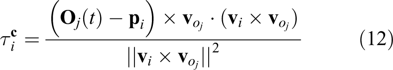
To cope with the inaccurate motion prediction of a dynamic obstacle, when the dynamic obstacle’s predicted trajectory moves across the predicted robot’s trajectory, we adopt the moving trends of the robot and dynamic obstacles to evaluate the collision possibility. Therefore, we create a trend-aware method to detect the potential collision.

For every configuration of the predicted trajectories of the robot and dynamic obstacles, we project the moving trends based on its own orientation or velocity’s direction

$\{\begin{array}{l}\mathbf{C}\left({\tau }_i^{\mathbf{c}}\right)={\mathbf{p}}_i+{\mathbf{v}}_i{\tau }_i^{\mathbf{c}}\hfill \\ {\mathbf{O}}_j\left({\tau }_i^j\right)={\mathbf{O}}_j(t)+{\mathbf{v}}_{{\mathbf{O}}_j}{\tau }_i^j\hfill \end{array}$

8

where the predicted position of the robot is denoted as ${\mathbf{p}}_i$ which consists of x_i and y_i . ${\mathbf{v}}_i$ represents the velocity of the robot. ${\tau }_i^{\mathbf{c}}$ and ${\tau }_i^j$ are the trend parameters of the robot and the jth dynamic obstacle, respectively, and both the trend parameters determine the size of the trend. $\mathbf{C}\left({\tau }_i^{\mathbf{c}}\right)$ and ${\mathbf{O}}_j\left({\tau }_i^j\right)$ represent the trend state of the robot and the jth dynamic obstacle, respectively, and a sequence of trend states constitutes a trend trajectory.

When the distance between the configurations of the robot and dynamic obstacles is close enough, the trend projection mentioned above will engage. The distance between the configurations of the robot and the jth dynamic obstacle is computed as

$\delta \left({\mathbf{c}}_i,{\mathbf{O}}_j\left(t\right)\right)={\Vert {\mathbf{O}}_j\left(t\right)-{\mathbf{p}}_i\Vert }_2$

9

A modified sigmoid function is implemented on the distance result

$\gamma =\frac{1}{1+e^{\kappa }{ }^{[\delta ({\mathbf{c}}_i,{\mathbf{O}}_j(t))-{\delta }_{\text{req}}]}}$

10

where $\gamma \in [0,1]$ is the conditional judgment, ${\delta }_{\text{req}}$ is given an empirical value, and $\kappa$ denotes a scaling factor.

When γ is unequal to zero, it means the existence of the dynamic obstacle is threatening the safety of the robot. Hence, the collision detection is implemented. First it is necessary to compute ${\mathbf{v}}_i\times {\mathbf{v}}_{o_j}$ for ensuring whether the trend trajectories of the robot and jth dynamic obstacle are neither paralleled nor colinear. Once the trend trajectories are neither paralleled nor colinear, the detection of a collision is computed by detecting the trend trajectories’ intersection

$\mathbf{C}\left({\tau }_i^{\mathbf{c}}\right)={\mathbf{O}}_j\left({\tau }_i^j\right)$

11

${\tau }_i^{\mathbf{c}}=\frac{\left({\mathbf{O}}_j\left(t\right)-{\mathbf{p}}_i\right)\times {\mathbf{v}}_{o_j}\cdot \left({\mathbf{v}}_i\times {\mathbf{v}}_{o_j}\right)}{{\Vert {\mathbf{v}}_i\times {\mathbf{v}}_{o_j}\Vert }^2}$

12

${\tau }_i^j=\frac{\left({\mathbf{p}}_i-{\mathbf{O}}_j\left(t\right)\right)\times {\mathbf{v}}_i\cdot \left({\mathbf{v}}_{o_j}\times {\mathbf{v}}_i\right)}{{\Vert {\mathbf{v}}_{o_j}\times {\mathbf{v}}_i\Vert }^2}$

13

If ${\tau }_i^{\mathbf{c}}$ or ${\tau }_i^j$ is greater than or equal to zero, we consider that there is a potential collision between the robot and the jth dynamic obstacle. The possibility of collision can be greatly reduced if the trend constraint σ_i is satisfied, and the trend constraint σ_i is defined as

$\begin{array}{c}{\sigma }_i={\left[{\sigma }_{\text{min}},{\sigma }_{\text{min}},\mathrm{...},{\sigma }_{\text{min}}\right]}^T\\ -{\left[{\tau }_i^0,{\tau }_i^1,\mathrm{...},{\tau }_i^j\right]}^T\ge 0\end{array}$

14

where σ _min is denoted as a minimal intersection distance to maintain the safe clearance between the robot and the jth dynamic obstacle.

The constraints of TATD are built and ready for trend-aware trajectory optimization.

Robotic fundamental constraints

The robot’s kinematics and dynamics are the fundamental components for local motion planning, and a stable and reliable trajectory optimization method needs to subject to the following constraints

$\begin{array}{c}{h}_i\left({\mathbf{c}}_{i+1},{\mathbf{c}}_i\right)=0,(\text{non−holonomic kinematics})\\ {\nu }_i\left({\mathbf{c}}_{i+1},{\mathbf{c}}_i,\Delta t_i\right)\ge 0, \hspace{0.17em}\hspace{0.17em}\hspace{0.17em}\hspace{0.17em}\hspace{0.17em}\hspace{0.17em}\hspace{0.17em}\hspace{0.17em}(\text{velocity bound})\\ {\alpha }_i\left({\mathbf{c}}_{i+1},{\mathbf{c}}_i,{\mathbf{c}}_{i-1},\Delta t_{i+1},\Delta t_i\right)\ge 0,\hspace{0.17em}\hspace{0.17em}\left(\text{acceleration bound}\right)\end{array}$

where $h_i$ represents the non-holonomic kinematics constraint and ${\nu }_i$ and ${\alpha }_i$ represent the dynamics constraint.

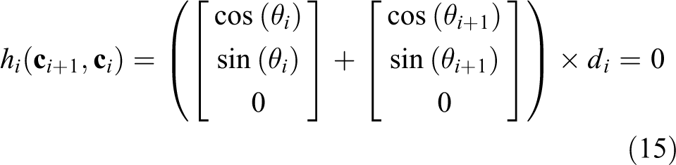
As is mentioned above, the robot uses a differential model. The robot’s motion control only has two degrees of freedom. The non-holonomic kinematics constraint requires that the robot’s two adjacent configurations ${\mathbf{c}}_i$ and ${\mathbf{c}}_{i+1}$ are located on a common arc of constant curvature. Let ${\beta }_i$ represent the angular difference between the robot’s configuration ${\mathbf{c}}_i$ and its motion direction $d_i={\left[x_{i+1}-x_i,y_{i+1} -y_i,0\right]}^{\text{T}}$ ; similarly, ${\beta }_{i+1}$ represents the angular difference between the robot’s configuration ${\mathbf{c}}_{i+1}$ and the motion direction $d_i$ . Only if both the angular differences ${\beta }_i$ and ${\beta }_{i+1}$ are equal, the common arc of the constant curvature can be obtained. The non-holonomic kinematics constraint is defined as

$h_i\left({\mathbf{c}}_{i+1},{\mathbf{c}}_i\right)=\left(\left[\begin{array}{c}\text{cos}\hspace{0.17em}\left({\theta }_i\right)\\ \text{sin}\hspace{0.17em}\left({\theta }_i\right)\\ 0\end{array}\right]+\left[\begin{array}{c}\text{cos}\hspace{0.17em}\left({\theta }_{i+1}\right)\\ \text{sin}\hspace{0.17em}\left({\theta }_{i+1}\right)\\ 0\end{array}\right]\right)\times d_i=0$

15

The dynamical constraint is implemented for limiting the velocity and acceleration of the robot. The mean translational and rotational velocities are computed according to the Euclidean or angular distance between two consecutive configurations ${\mathbf{c}}_i$ , ${\mathbf{c}}_{i+1}$ and the time interval $\Delta t_i$

${\mathbf{v}}_i\simeq \Vert \left(\begin{array}{l}{x}_{i+1}-x_i\\ y_{i+1}-y_i\end{array}\right)\Vert \frac{1}{\Delta t_i}$

16

${\omega }_i\simeq \frac{{\theta }_{i+1}-{\theta }_i}{\Delta t_i}$

17

The velocity constraint is defined as

${\nu }_i\left({\mathbf{c}}_{i+1},{\mathbf{c}}_i,\Delta t_i\right)={\left[{\mathbf{v}}_{\text{max}}-|{\mathbf{v}}_i|,{\omega }_{\text{max}}-|{\omega }_i|\right]}^T\ge 0$

18

where ${\mathbf{v}}_{\text{max}}$ and ${\omega }_{\text{max}}$ are the maximum translational and rotational velocities of the robot, respectively.

The acceleration $a_i$ is related to two consecutive translational velocities ${\mathbf{v}}_i$ and ${\mathbf{v}}_{i+1}$ . Thus, the acceleration $a_i$ is computed as

$a_i=\frac{2\left({\mathbf{v}}_{i+1}-{\mathbf{v}}_i\right)}{\Delta t_i+\Delta t_{i+1}}$

19

The acceleration constraint is defined as

${\alpha }_i\left({\mathbf{c}}_{i+1},{\mathbf{c}}_i,{\mathbf{c}}_{i-1},\Delta t_{i+1},\Delta t_i\right)=a_{\text{max}}-|a_i|\ge 0$

20

where $a_{\text{max}}$ is the minimum acceleration of the robot.

Trajectory optimization

To acquire the optimized robot trajectory, the multi-objective optimization problem mentioned above is mapped into an approximative nonlinear squared optimization problem. The trend constraint is represented in terms of the quadratic penalty with weight $w_{\sigma }$

$w_{\sigma }{f}_{\sigma }\left(P\right)={\displaystyle \sum _{i=0}^{n-1}{w}_{\sigma }{\Vert \text{min}\left\{0,{\sigma }_i\right\}\Vert }_2^2}$

21

where $f_{\sigma }\left(P\right)$ is the trend objective function. Additional constraints $h_i$ , ${\nu }_i$ , and ${\alpha }_i$ are represented in a similar fashion.

The optimal trajectory $P^{\ast }$ is obtained by solving the approximated optimization problem

$\begin{array}{l}\mathbf{P}*=\text{arg}\underset{P\backslash \{{\mathbf{c}}_0,{\mathbf{c}}_n\}}{\text{min}}{\mathbf{w}}^{T}f\left(\mathbf{P}\right)\hfill \\ {\mathbf{w}}^{T}f\left(\mathbf{P}\right)={\displaystyle \sum _{i=0}^{n-1}{[w_{\sigma }\Vert \text{min}\left\{0,{\sigma }_i\right\}\Vert }_2^2}\hfill \\ \hspace{1em}\hspace{1em}\hspace{1em}\hspace{1em}+w_{\mathbf{z}}{\Vert \text{min}\left\{\mathbf{0},{\mathbf{z}}_i\right\}\Vert }_2^2+w_{\alpha }{\Vert \text{min}\left\{\mathbf{0},{\alpha }_i\right\}\Vert }_2^2\hfill \\ \hspace{1em}\hspace{1em}\hspace{1em}\hspace{1em}+w_{\mathbf{v}}{\Vert \text{min}\left\{\mathbf{0},{\mathbf{v}}_i\right\}\Vert }_2^2+w_h{\Vert {\mathbf{h}}_i\Vert }_2^2+\Delta t_i^2\hfill \end{array}$

22

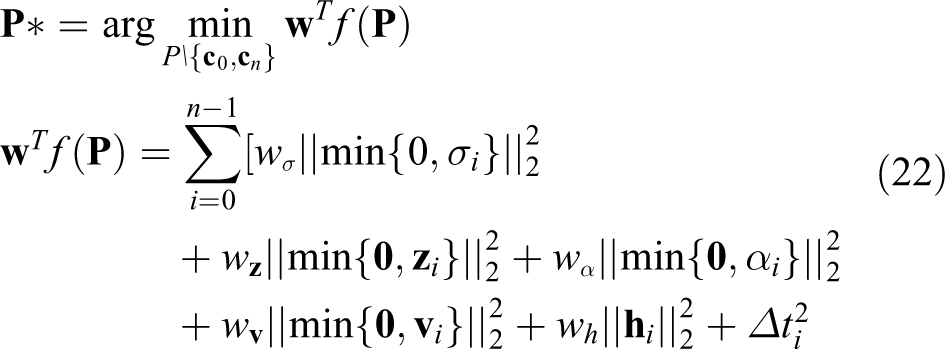
where objective function $f\left(P\right)$ contains all individual objective functions, $w^T$ denotes a weight vector which consists of all weight factors, and the total transition time is approximated by ${\displaystyle {\sum }_{i=0}^{n-1}\Delta t_i^2}$ .

As is depicted in Figure 2, the trajectory optimization problem is transformed into a hyper-graph that has configurations and time intervals as vertices. The edges are connected by the vertices, representing objective functions or constraint functions. The formulation (22) is solved by a sparse variant of the Levenberg–Marquardt algorithm which is utilized by the graph optimization framework g2o. ²⁹ The optimization of the trend objective function moves the vertices of the robot’s configurations away from the predicted obstacle states. Meanwhile, it deforms the vertices into a curve shape that avoids the moving trends of obstacles with the lowest cost.

Figure 2.

Simplified example of TATD hyper-graph with a circle-shaped moving obstacle, two configurations, and a time interval. The moving obstacle’s position varies in time but is a fixed vertex, which means its current position is not a variable and cannot be affected by the optimization procedure. Edge τ_i connects two vertices, and it represents the objective function which contains trend and distance constraint. TATD: trend-aware trajectory deformation.

Experiments and analysis

In this section, to demonstrate the advantages of our TAMP algorithm, we ran simulations in the presence of the multiple moving obstacles. We compare TAMP with TEB and TEB + HC. The three planners have the same kinematic and dynamic constraints, however, TAMP is different from the other planners in dealing with dynamic obstacle. The trajectories generated by the local motion planners are implemented to control the mobile robot motion directly. The local motion planners need to generate and deform trajectories consecutively based on the given global path so that the robot can reach the desired goal in case of the unexpected moving obstacles. Algorithms are performed on a PC with a 3.7-GHz Intel i7 CPU and 32 GB RAM.

It is worth mentioning that TAMP, TEB, and TEB + HC are implemented on the same non-holonomic mobile robot with the same parameter configuration.

Vertical crossing obstacles scenario with precise state estimation

In this scenario, to compare the performance of the three different motion planners, the robot starts from the same starting point at the same time and reaches the same end point by avoiding dynamic obstacles. The obstacles deployed the same and their accelerations are the same. The obstacles are moving vertically with constant acceleration. The precise states of the obstacles are given, and the motion planners perform online trajectories generation for the incoming obstacles based on the given data. As is shown in Figure 3, there are three frozen moments of each planner, which is time stamp 1, time stamp 2, and time stamp 3. The three time stamps represent that each planner generates a trajectory three times. Each planner’s time stamp 1 represents the first responding to an approaching dynamic obstacle. The last two time stamps show the follow-up response.

Figure 3(a) to (c) indicates that TAMP deforms the generated trajectory to bypass the moving obstacle while avoiding the moving trend of the obstacle; furthermore, the smoothness and stability of the trajectory are guaranteed. According to the simulation, the constantly changing speed of the obstacle has little effect on the shape of the trajectory. In contrast, Figure 3(d) to (f) shows that TEB tries to plan a trajectory to avoid the obstacle despite of its moving trend due to the current low speed of the obstacle, however, when the obstacle is accelerating, which force TEB to change the original plan continuously. The changing process is disturbing for the robot controller and might cause a collision with other obstacles. TEB + HC plans multiple trajectories in Figure 3(g) to (i) based on Voronoi diagrams and chooses the least cost one. Nevertheless, this method introduces a new dilemma that the cost of each alternative trajectory is variable due to the unstable obstacles, which leads to a disturbing result.

The performance of TAMP shows that although TAMP is using the constant motion model for dynamic obstacles motion prediction, it is still robust to avoid the moving trends of the dynamic obstacles with constant acceleration and maintain the minimum cost.

Slant crossing obstacles scenario with disturbed state estimation

The following experiment compares several metrics to evaluate the attribute of the approaches. Due to the uncertainty of the dynamic obstacles, we measure the whole process that the non-holonomic robot bypasses the moving obstacles until it reaches the target configuration instead of a partial process within a short time horizon. Hence, the safety and global optima can be quantified. We evaluate the performance of three methods by several metrics.

The traveled path shows the complete path length from the start to the end, which indicates the odometry cost of avoiding dynamic obstacles.

The consumed time directly reveals the efficiency of the planner, which implies the average speed of the robot is higher or lower.

The translational velocity profile shows the stability of the robot controlled by the motion planner, which implies how smooth the planned trajectory is.

When the moving obstacles are crossing in front of the robot unexpectedly and blocking the original trajectory of the robot, a retreat behavior might be triggered to keep the robot away from a collision threat. A retreat behavior has a primary influence on trajectory smoothness, which pursuits safety for avoiding unexpected moving obstacles. The frequency of retreat behavior can be reduced by implementing a better motion planner.

Figure 3.

The planning moment of (a) to (c) TAMP, (d) to (f) TEB, and (g) to (i) TEB + HC are depicted. The dynamic obstacles are moving vertically with constant acceleration. The planners need to generate collision-free trajectories for the robot to handle the situation safely. (a) Time stamp 1. (b) Time stamp 2. (c) Time stamp 3. (d) Time stamp 1. (e) Time stamp 2. (f) Time stamp 3. (g) Time stamp 1. (h) Time stamp 2. (i) Time stamp 3. TEB: timed elastic band; HC: homology class.

In the experiment, the dynamic environment is deployed as a 25 × 6 m² grid map with 14 obstacles which are moving along specific trajectories with constant acceleration. When the speed of the obstacles reaches the upper limit or zero, the acceleration will change the current sign. A random disturbance is applied to the dynamic obstacles’ velocity estimation so that the planners cannot rely on the motion prediction of the dynamic obstacles. When the dynamic obstacles reach the bottom or top of the grid map, their vertical movement directions will be reversed. The planning complexity is increased massively in this scenario. The initial configuration and the final destination are set at feasible locations in the grid map, respectively. All the planners are given a feasible path straight to the goal without colliding with static barriers. Moreover, the planners are initialized at the same moment. The maximum linear and angular velocities of the mobile robot are limited to 0.4 m/s and 0.6 rad/s, respectively.

Figure 4 depicts that three complete simulations implementing different methods, respectively, in one environment to show the exact state of the robot controlled by the planners. The three different lines represent the traveled paths of the robot implementing the three different methods. The red and green lines are not smooth, which means retreat behaviors are triggered. TAMP constantly seeks a more feasible and smoother piecewise path instead of being blocked by the obstacles and having to proceed with a retreat behavior. And TAMP always avoids the moving trends of the dynamic obstacles such that the influence of the inaccurate obstacles’ motion prediction is minimized. Therefore, TAMP results in generating foresighted evasive maneuvers. As giving the random disturbance to the obstacles’ velocity value, TEB and TEB + HC can only deal with the imminent crossing obstacle, however, TAMP already takes actions about the obstacles at the end of the planning horizon, which maintains the relatively long-term solution robustly and optimizes the trajectory efficiently.

Figure 4.

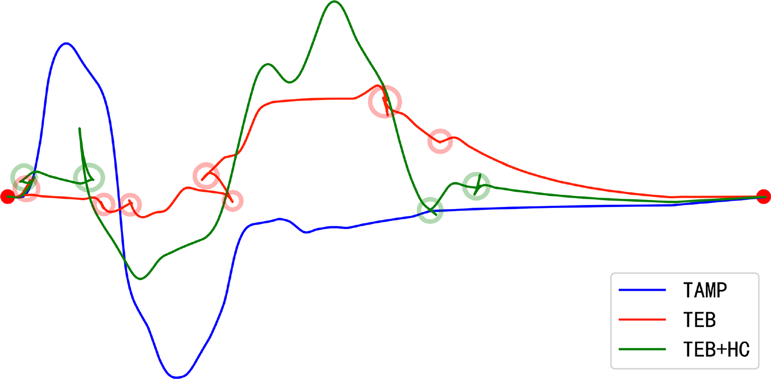
Traveled paths of the robot implementing the three different methods. The red dots represent the start and goal points. The red and green circular markers on the paths suggest that retreat behaviors are executed because of the slant crossing obstacles. The paths’ length of TAMP (blue line), TEB (red line), and TEB + HC (green line) are 23.36 m, 25.88 m, and 25.62 m, respectively. TEB: timed elastic band; HC: homology class.

Then each planner is executed 10 times repeatedly for the same challenging scenario in which the dynamic obstacles’ orientation provided to each planner may reach a deviation of 40°. It is illustrated in 5(a) that TAMP outperforms other methods in maintaining higher velocities of the robot and the outliers of TAMP are barely negative. As is shown in Table 1, the interquartile range of TAMP’s velocity is lower than other methods, which means smoother and control-friendly trajectories are generated iteratively. The poor quality of the obstacles’ motion prediction causes TEB and TEB + HC to oscillate easily. As is shown in Figure 5(b) and (c), TEB and TEB + HC take more detours than TAMP, which lead to longer path and time consumption. And their results are scattered in a relatively large range, which implies that TAMP is more stable than other methods. The standard deviation in Table 1 can also demonstrate that every attempt of TEB and TEB + HC in completing the experiment is more probabilistic than TAMP. The sudden change in the moving direction of the robot brings major pressure into the hardware of the robot. The results highlight that TEB and TEB + HC have more trouble in dealing with the slant crossing obstacles with poor state estimation, while TAMP can guide the robot slips out of the dynamic dilemma.

Table 1.

The metric data for the methods to compare with velocity v, path length l, and time consumption t are depicted in Figure 5.

Approach	Metric	Mean	Standard Deviation	Minimum	Lower Quartile	Median	Upper Quartile	Maximum
TAMP	v (m/s)	0.3595	0.0582	−0.2	0.3655	0.3735	0.3818	0.4
	l (m)	23.5733	0.4201	23.0691	23.353	23.4755	23.5863	24.5208
	t (s)	65.3428	1.6135	64.1018	64.281	64.6095	65.5142	68.7331
TEB	v (m/s)	0.2747	0.186	−0.2	0.2834	0.3685	0.3733	0.4
	l (m)	26.309	1.2287	24.5736	25.2751	26.6918	26.9924	28.1734
	t (s)	82.521	7.2222	71.5432	77.0304	82.5075	88.0979	92.8645
TEB + HC	v (m/s)	0.2761	0.1811	−0.2	0.274	0.3693	0.3731	0.4
	l (m)	25.1731	0.7806	24.2249	24.6693	24.9931	25.4383	26.5306
	t (s)	79.3848	4.6802	74.3327	76.6969	77.2139	81.3022	90.2636

TEB: timed elastic band; HC: homology class.

Figure 5.

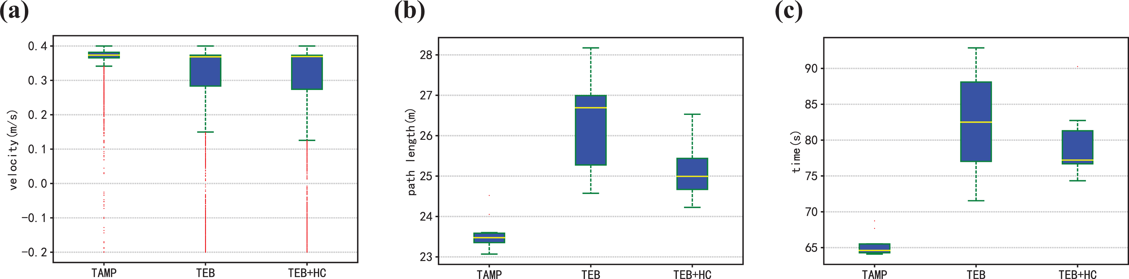
Comparison between approaches. The red dots on (a) are the outliers of the major velocity. When the outliers are less than zero, the robot is retreating for avoiding a collision. The detailed data are presented in Table 1: (a) velocity profile (m/s), (b) path length (m), and (c) time consuming (s).

Conclusion

In this article, we proposed a novel approach for avoiding dynamic obstacles, called trend-aware motion planning (TAMP). For the purpose of guaranteeing the safety of the generated trajectory, TAMP is designed to deal with the dynamic obstacles under inaccurate motion prediction by taking the moving trends of the obstacles into account. TATD moves configuration vertices away from the moving obstacles’ future possible moving trends, and TAMP maintains the continuity and smoothness of the trajectory simultaneously. According to our experiments, TAMP generates more stable and safer trajectories and results in smaller path length and lower time consumption averagely than the state-of-the-art TEB and TEB + HC planners. In general, TAMP outperforms TEB and TEB + HC in dynamic environments with moving obstacles. Further work includes adding curvature constraints on TAMP and applying TAMP to three-dimensional space for micro aerial vehicles.