Sage Journals: Discover world-class research

Abstract

For an autonomous mobile robot operating in an unknown environment, distinguishing obstacles from the traversable ground region is an essential step in determining whether the robot can traverse the area. Ground segmentation thus plays a critical role in autonomous mobile robot navigation in challenging environments, especially in real time. In this article, a ground segmentation method is proposed that combines three techniques: gradient threshold, adaptive break point detection, and mean height evaluation. Based on three-dimensional (3D) point clouds obtained from a Velodyne HDL-32E sensor, and by exploiting the structure of a two-dimensional reference image, the 3D data are represented as a graph data structures. This process serves as both a preprocessing step and a visualization of very large data sets, mobile-generated data for segmentation, and building maps of the area. Various types of 3D data—such as ground regions near the sensor center, uneven regions, and sparse regions—need to be represented and segmented. For the ground regions, we apply the gradient threshold technique for segmentation. We address the uneven regions using adaptive break points. Finally, for the sparse region, we segment the ground by using a mean height evaluation.

Keywords

Mobile robot gradient field three-dimensional point cloud two-dimensional range image mean height evaluation

Introduction

Autonomous mobile robots are intelligent machines that are capable of acting on their own, sensing their surrounding environment, and independently performing tasks without explicit human control. An important objective of automation robotics research is to enable the robot to perceive and interpret terrain for safe movement and the ability to collect data, handle its processing, and compute in real time. To this end, a traditional approach is to use a digital camera for two-dimensional (2D) machine vision to capture images of objects, perform image preprocessing, and execute computer vision techniques to extract useful information. Nowadays, three-dimensional (3D) machine vision technology is most commonly used to provide more precise 3D inspection and measurement of complex 3D surfaces. The increased availability of new solutions has made these technologies more robust and easier to use, while opening new capabilities and presenting interesting challenges for 3D machine vision.

3D scanner data (point clouds) comprise a digitized model of the surrounding environment from 3D scanners. 3D point clouds are the output of 3D scanning processes and they are collected and used for many purposes. Through mobile data processing of 3D sensors, data are applied to mobile robotics sensors and to the Velodyne sensor, in particular, which is adopted in our autonomous mobile robot. The robot must identify and segment the traversable ground region and obstacles over which it cannot pass based on 3D point cloud preprocessing techniques, such as segmentations that separate the ground from obstacles, borders, and curbs.

Ground segmentation is therefore a crucial task and an essential step in other higher processes, such as 3D object recognition, classification, object tracking, and obstacle detection. Its objective is to extract useful information from 3D point cloud data, and then cluster points with similar properties into the same ground region. In addition, it provides mobile data processing techniques to autonomous mobile robots according to a real-time approach. This approach is defined as completing all mobile data processing routines before the next sensor data frame arrives.

Many ground segmentation methods exist for 3D point clouds. They can be roughly classified into two main categories: elevation map methods^1
–3 and geometric model fitting methods.^4

–7 These methods work relatively well with dense, flat 3D point clouds. However, it has difficulty contending with sparse noisy data, a challenge that needs to be addressed.

With a focus on data characteristics, a ground segmentation algorithm is herein proposed that employs specific 3D data as well as various terrains in real time. The algorithm is based on three combined techniques: gradient threshold segmentation,⁴ adaptive break point detection,⁷ and mean height evaluation. We apply each technique with various types of data in the abovementioned ground segmentation.

Related work

3D-scanning devices are becoming standard enterprise equipment for autonomous mobile robots. Many studies conducted in the last few years have focused on ground segmentation.^{2,4

–7,8

–23} Various research groups have proposed techniques for handling 3D point cloud data, not only in the spatial domain, but also in the frequency domain. We roughly categorize these techniques in relation to our present research in the subsections below.

Ground segmentation methods based on elevation maps

To address numerous points obtained by Lidar devices, an effective approach is to lower the data dimension. Elevation maps are 2.5-dimensional (2.5D) grids of values reflecting the different elevations, or altitudes, at different positions in world units. The main idea of this approach is mapping three dimensions to the 2.5D grid structure, whose third dimension is only partially modeled. Then, the height of the terrain is stored at the corresponding actual geometric position.

Thrun et al.¹ proposed reducing dimensionality by projecting the 3D points to a 2.5D grid. This method, called elevation-map min–max, was used by many teams at the 2006 Defense Advanced Research Projects Agency Urban Challenge robot competition. The method computes the difference between the maximum and minimum heights of 3D point clouds in a cell. An occupied cell is determined by the difference of height, which exceeds a predefined threshold. Otherwise, a cell is deemed a ground cell. Height differences supply approximations as an efficient means to obtaining the terrain gradient in a cell.

In the study by Douillard et al.,² 3D point cloud data are represented as a grid of values called a mean elevation map. Each value, the mean height, is computed by averaging the height of all points located in each grid cell. Identifying obstacles involves two main steps: (1) calculating the surface gradient and (2) applying a threshold. The extraction of the ground is a process by which cells are removed from the mean elevation map of protruding objects.

The efficient extension approach of the elevation map was proposed by Pfaff et al.³ The so-called multilevel elevation map enables the handling of overhanging structures.

Geometric model fitting methods

Geometric model fitting methods are used to process 3D data, especially to fit primitive shapes to 3D data based on fitting geometric primitive shapes. In this approach, there are two common shape types: a line and surface. Accordingly, 3D point clouds are represented as one segment if they have the same mathematical properties.

Himmelsbach et al.⁶ presented an approach for capturing the transition between flat and sloped terrain by considering the local surface properties. A polar grid map is employed to represent the xy-plane as a circle with an infinite radius. This circle is then divided into a finite number of segments. From that point, all points are mapped to one of the many bins to discretize the range of point components for each segment. This technique enables conversion of a set of 3D points to the same bin. A set of 2D points can thereby be obtained. A set of points, or no points, is called a prototype point, which is used for calculating all non-empty bin points. By applying an incremental algorithm, the ground plane line is extracted from the prototype set of each segment. Therefore, with each line describing the ground plane within one segment, all points identified in the segment are labeled as either belonging or not belonging to the ground plane.

In the study by Lam et al.,⁷ the 3D ground region is obtained by modeling the process as a dynamic system of connected planes. There are two key stages in this process. First, a 3D local plane that fits a bounded region of the 3D data is estimated based on applying the least squares fit on that 3D data. The random sample consensus method is used to eliminate the outliers. Second, the road is globally extracted by smoothly connecting each local plane. In addition, a Kalman filter is employed to predict and find the subsequent locations of the previous local plane on the same road. The Kalman filter has been used in different prediction applications and vision tracking.

Thrun et al.¹ proposed two algorithms to handle sparse data. Gaussian process incremental sample consensus is an algorithm that operates on the sparse 3D data. It is also known as probabilistic, continuous ground surface estimation. This algorithm fits a geometric model from a single seed of high probability inliers. It then evaluates the remaining data points. The other algorithm is mesh-based segmentation. First, the mesh of the received data is created based on exploiting the structures of the scanning process. The mesh cannot be captured with a constant grid if the received data are sparse. A gradient feature of each point is used to calculate from the mesh. As a result, by using a specific region-growing technique, the ground partition is expanded from a seed region through the connected topology.

A similar method is presented by Moosmann et al.⁵ to construct the mesh from 3D data by analyzing the scanning process structure. Another method is applied to extract the ground region. Moosmann et al.⁵ proposed a criterion, called local convexity, to segment 3D data. The criterion uses local geometric features. The local surface around a point is approximated by a plane or its normal vector. Two neighboring surfaces are combined as a segment if they are locally convex to each other or if their normal vectors are in approximately the same direction.

The above studies motivated our proposal of a ground segmentation algorithm using a combination of three techniques. This combined approach enables our algorithm to work with various 3D data in real time. First, we employ the gradient-field-based approaches in the study by Douillard et al.⁴ Second, the 3D point cloud is represented as a graph by exploiting the structure of a 2D reference image received from the scanning process, as in the study by Moosmann et al.⁵ Third, two adaptive methods are included to handle noisy, sparse data.

Data representation for a 3D point cloud

In this section, to illustrate our 3D point cloud, we discuss the graph data structure and describe its characteristics. The structure is built using a 2D reference image, as explained earlier.

Graph representation based on a 2D reference image

In this study, 3D point clouds obtained from a Velodyne HDL-32E were transformed into a 2D reference image with a size of 32 × 2160. The horizontal axis was scanned by a laser scanner to obtain a horizontal scan line (one laser diode). It contained a maximum of 2160 data points per line. Thirty-two vertical scan lines were acquired (32 laser diodes). All 3D point clouds were referenced by using the 2D image. Figure 1 shows the representation. The right-hand Cartesian coordinate system depicts our 3D system. The y-coordinate determines the height of the points; the z-direction represents the movement of autonomous mobile robots.

Figure 1.

Data mapping to a 2D reference image. 2D: two-dimensional.

To formalize the problem, let the 2D reference image be an undirected graph G(E, V, w). We call V = {pⁱ(w, h)} a set of vertices, (w, h) is the coordinate of vertex pⁱ in 2D image which references to a measured point in 3D point cloud, E = {(pⁱ, p^j)} is a set of edges connecting two vertices, and w: E → R is a weight function that maps each edge in set E to a real number. To determine the weight of an edge, we calculate the distance between two verticals of the edge according to the Euclidean distance formula as follows

w [(p^{i}, p^{j})] = | | p^{i} - p^{j} | |

Figure 2 shows the graph representation as meshes. Figure 3 depicts these meshes as constructed by connecting points to the neighbors based on the 2D reference image.

Figure 2.

Meshes constructed from good data.

Figure 3.

Meshes built from noisy data.

As shown in Figure 2, the mesh is built from a dense, almost flat 3D point cloud. In this graph, nearly all edges have a reasonable weight (the distance between two 3D points), and the orders of all scan lines are the same.

In Figure 3, a graph mesh is illustrated in noisy, sparse 3D data. The quality is poor and the mesh is rough. These issues occur owing to noise points, and padding points automatically fill in the scanning process.

Properties and characteristics

In accordance with the graph representation in “Graph representation based on a 2D reference image” section, each point in the 3D point cloud has a maximum of four neighbors. In the counterclockwise system, a point’s left neighbor corresponds to the next measurement obtained by the same laser diode, while its right neighbor corresponds to the previous measurement. The upper and lower edges are assigned to the measurements of the upper and lower laser beams with the most similar yaw angle, respectively. To more clearly illustrate this concept, each point pⁱ(w, h) has a maximum of four neighbors: $p_{l}^{i}$ (w − 1, h), $p_{r}^{i}$ (w + 1, h), $p_{d}^{i}$ (w, h − 1), and $p_{u}^{i}$ (w, h + 1), as shown in Figure 4. The subscript denotes the neighbor’s direction (left, right, up, and down).

Figure 4.

Neighbors in a 2D image. 2D: two-dimensional.

Basically, the four neighbors in the above graph representation need not be the nearest neighbors in a 3D environment. Nonetheless, the distances between them must be reasonable. Although the graph shows a simple and effective representation, it has two key disadvantages, as described below.

In the case in which the sensor does not obtain the returning laser beam, padding data with values (0, 0, 0) are inserted into the position presented for that beam. These positions must be equivalent to infinity points in the real world. The values at these positions themselves do not make sense. They must be removed when we build the graph. These padding points are removed based on calculating the weights of particular edges in the graph. They are compared them with a predefined threshold value, reasonDst. If the weight of a particular edge is greater than reasonDst, this edge is removed.

In the case of two consecutive data lines generated by two consecutive laser diodes, the order is reversed. To resolve this problem, we choose a potential edge connecting two initial points belonging to each line, and another potential edge that connects the first and last points of two consecutive lines. If their weight difference is greater than a threshold value, reasonDst, we sort the order of these scan lines.

Another problem also occurs with noisy points. In the scanning process of the rescue, noisy points are generated when the fired laser beam reaches any part of the robot and bounces back. If only the weight information of the graph is used, it is not easy to remove noisy points. Hence, we must analyze the characteristics of the sensing devices and the scanning process structure.

Creating the 3D point cloud graph representation is the first step of our algorithm. It provides an improved approach to obtaining and processing the data. It is the premise for all subsequent steps of our works. In “Experimental results and analysis” section, we illustrate the different results of using different graph representations with the same 3D point cloud.

Adaptive ground segmentation method

In this section, we detail our proposed algorithm that is used for segmentation from 3D point clouds. First, we present gradient field calculation⁴ and adaptive break point detection techniques.²⁴ Second, we describe the mean height evaluation technique, which is included in our final algorithm and is discussed in “Ground segmentation method based on the gradient field” section.

Gradient field calculation

The gradient quantity is a significant feature in three dimensions. Fundamentally, the gradient represents the slope of the tangent line of the graph of the function. It is a vector (the direction in which to move). Specifically, the gradient points are situated in the direction of the greatest rate of increase in the function. The magnitude is the slope in that direction. Determining the gradient is usually achieved by calculating the function differentiation.

Precisely, if $f (x_{1}, \dots, x_{n})$ is a differentiable function in Euclidean space, the gradient is the vector whose components are the n partial derivatives of the f function. In the 3D Cartesian coordinate system, the gradient of function f(x, y, z) is given by

gradf (x, y, z) = Δ f (x, y, z) = (\frac{d f}{d x}, \frac{d f}{d y}, \frac{d f}{d z})

Using this approach, interpolating a surface from neighbors of a 3D point is typically time-intensive.

Figure 5 illustrates the method to calculate the gradient of point pⁱ of the right direction. We trace to pⁱ according to the right direction to determine the neighbors. We then sum all the distances until obtaining the mindst threshold distance value

d (p^{i}, p^{i}^{+ 1}) + d (p^{i}^{+ 1}, p^{i}^{+ 2}) + \dots + d (p^{j}^{- 1}, p^{j}) \leq m i n d s t

Figure 5.

Right direction gradient calculation.

The gradient of the direction of pⁱ is calculated as

g_{r}^{i} = \frac{abs (p_{r}^{i} . y - p_{r}^{j} . y)}{| | p^{i} - p^{j} | |}

where $g_{r}^{i}$ is the gradient value of point pⁱ of its specific direction, p^j is the furthermost point from pⁱ where we obtain the mindst threshold value, and $abs (p_{r}^{i} . y - p_{r}^{j} . y)$ gives the height difference between pⁱ and p^j .

Nonetheless, the gradient of a given direction is ignored if the mindst length is not covered in that direction in some points, because the points occur near the boundaries. Figure 6 depicts the issue of which we cannot cover the mindst of the downward direction of point p. To remove the noisy points of our 3D point cloud, whereby we cannot reach adequately far in every direction, we apply a distance threshold.

Figure 6.

Ignored direction example.

To produce a better result in some particular situations, we choose two consecutive points in a specific direction that have a maximum height difference over their distance. More precisely, we calculate the gradient of each direction as follows

g_{r}^{i} = max (\frac{abs (P_{r}^{k} . y - P_{r}^{k + 1} . y)}{d (P_{r}^{k}, P_{r}^{k + 1})})

As a result, the maximum gradient value of all directions is the gradient of a 3D point cloud (left, right, up, and down).

grad (p^{i}) = max (g_{l}^{i}, g_{r}^{i}, g_{u}^{i}, g_{d}^{i})

Adaptive break point detection

Break points relate to points in which discontinuities are detected in the scanning process due to obstacles or changes of the surface by the laser scanner. We can avoid connecting two neighboring linear clusters by applying the break point detection. Moreover, we employ this method for confusing points near the boundaries of segmented ground regions.

In naïve break point detection, if the distance between two consecutive points, pⁿ and p^{n − 1}, is greater than a predefined threshold, D _max, then the two points are set as a break point. In a real situation, it is not easy to calculate the D _max value. Furthermore, it is unreasonable to apply all points with only one threshold value in the 3D point cloud.

An improved method is proposed by Borges and Aldon²⁴ to calculate the D _max value. The D _max value is recalculated at every point in the line.

Figure 7 depicts the method of calculating the D _max value for the p^{i − 1} point. At the p^{i − 1} point, we create a virtual line. The line forms angle λ with respect to the line from the p^{i − 1} point to the origin. Here, λ is a predefined threshold value based on the characteristic of the sensor, and r^{i − 1} is the Euclidean distance from point p^{i − 1} to the origin. In addition, Δϕ is the difference between two angles created by two lines from the origin passing through points pⁱ and p^{i − 1}. The D _max value with respect to a point is calculated as follows

D_{max} = \frac{r^{i - 1} \times sin (Δ ϕ)}{sin (λ - Δ ϕ)}

Figure 7.

Adaptive break point detection.

If $| | p^{n} - p^{n - 1} | | > D_{max}$ , then both pⁿ and p^{n − 1} are set as a break point. Algorithm 1 presents the implementation of adaptive break point detection.

Algorithm 1.

Adaptive break point detection.

1 b[1] = false

2 for i = 2 to n

D_{max} = \frac{r^{i - 1} \times sin (Δ ϕ)}{sin (λ - Δ ϕ)}

4 if(||

p^{n} - p^{n - 1} | | > D_{max}

)

5 b[i] = true

6 b[i − 1] = true

7 else

8 b[i] = false

9 end if

10 end for

Because the D_max value at each point is recalculated, it only depends on its related information. Therefore, this technique is more effective than the naïve method.

Ground segmentation method based on the gradient field

In this research, we concentrate on segmentations of various types of terrain. To present our ground segmentation algorithm, we divide it into four stages. First, we calculate the gradient field of the 3D point clouds. Second, to segment the ground region near the sensor’s position, we apply the region-growing technique. Third, we apply the adaptive break point detection at confusing points near boundaries to determine whether these points belong to the ground. Finally, to analyze the difference between the height of the considered point and its indirect neighbors, some of which are already marked as ground points, we apply the so-called mean height evaluation technique. A point is marked as ground if the value is in the range of a threshold value.

To begin with the calculation process, two assumptions are required. (1) The ground is observed around the sensor. In addition, the sensor is mounted on the robot head or top of the vehicle, which moves on the ground. Assume that we know the position of the sensor, and the ground is observed around this position. (2) The minimum part of the closest line of data from the lowest laser diode falls on the ground region. The technique is used to segment the ground region in the second stage. The two above assumptions are illustrated in Figure 8.

Figure 8.

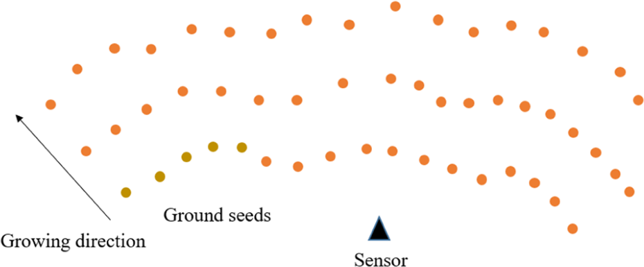
Region-growing assumptions.

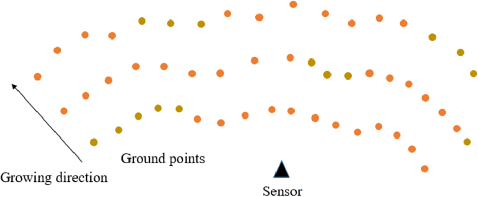
From a set of seeds, it examines all the neighbors and then determines whether neighbors should be added to the region. The longest sequence of the point belongs to the nearest line whose gradient values do not exceed the maxgrad threshold value, which is seed S₀. Its value is predefined and depends on the terrain properties. For a sequence, S_k, of the closest line, we evaluate the heights of the two closest points that belong to two sequences, S₀ and S_k, that should not exceed the maxdh value. All points of S_k are marked as ground points. Considering other scan lines, we can determine whether the ground region is grown from these seed points. The gradient value at a point is below maxgrad; thus, a point is marked as ground. The minimum one of its direct neighbors is already marked as a ground point.

In the experiment, we applied the recursive method for Algorithm 2. However, it resulted in a stack overflow error because of the massive number of points in the 3D point cloud and the memory growth at an exponential rate. Therefore, we applied the stack data structure to overcome this issue. The pseudo-code of the ground region growing stage using the stack structure is presented in Algorithm 2.

Algorithm 2.

Grounding growing technique.

1 S:stack

2 S.push(seeds)

3 while(S not empty)

4 N = S.pop()

5 for Nb ⊂ {N.neighbors()}

6 if(Nb.ground == false && Nb.gradient() < maxgrad)

7 Nb.ground = true

8 S.push(Nb)

9 end if

10 end for

11 end while

The gradient threshold technique works well only for dense flat regions near the position of the sensor. Two problems arise when the distance from the origin increases. (1) Typically, if a small obstacle is located on the ground, a significant difference does not exist between the gradient of points representing the obstacle and the ground points near it. Hence, the ground segmentation result is over-segmented with this obstacle when we only apply the gradient threshold technique. (2) The under-segmented problem occurs when the terrain has uneven parts. The two problems above are illustrated in Figure 9.

Figure 9.

Confusing points.

In Figure 9, point pⁱ belongs to the ground region and point p^j may belong to a particular small object. However, according to the method we used by applying only the gradient threshold technique with a particular maxgrad threshold value, p^j is marked as a segmented ground point or pⁱ is marked as segmented non-ground points. They appear to have the same gradient value. Therefore, it may be confusing to decide whether p^j belongs to the ground.

To address this problem, we check all the boundary points of the segmented ground using the adaptive break point detection technique. As a result, the ground is refined.

Nevertheless, the adaptive break point detection as discussed in “Adaptive break point detection” section only works on a 2D plane. We thus must map our 3D points to a 2D plane by projecting them on a (y-, z-axis) local plane (in our system), as shown in Figure 10. Then, we apply adaptive break point detection at all pairs of consecutive points of the same scan line (one of which is already marked as a ground point). We check if there is no discontinuity between the ground and non-ground neighbor point and mark the neighbor point as a ground point without regard for its gradient value. For simplicity, we only check the consecutive points on the same scan line.

Figure 10.

Adaptive break point checking.

All points on a specific scan line are projected onto a 2D (y-, z-plane), as shown in Figure 10. pⁱ is not marked as a ground point, because there is a discontinuity between pⁱ ^{− 1}, a ground point, and pⁱ according to the adaptive break point detection method when verifying point pⁱ ^{− 1}.

When the distance between the scanned objects and the origin increases, the collected 3D point cloud gradually becomes sparse. In these sparse regions, the region-growing technique does not work well, as explained in “Gradient field calculation” section. The points with gradient values below threshold maxgrad do not remain on consecutive scan lines (vertical), nor do they remain consecutively on the same line (horizontal). Therefore, we determine that they are not neighbors. For the final stage, our algorithm uses the mean height evaluation to segment the ground point in these sparse regions.

As shown in Figure 11, yellow point regions have gradient values below threshold maxgrad, and some of them are marked as ground. We call these points segmented ground points. No connection exists between these regions; thus, the region-growing technique does not work. To handle this problem, we consider in detail 3D points in the predefined region. The height of every segmented ground point is compared with the mean height of every ground point inside that region. If the difference does not exceed a threshold maxdh value, as mentioned, then we mark them as the ground. We illustrate this technique in Figure 12. Assume that a region is a rectangle with reasonable sizes. These sizes are chosen according to the sparse level of the 3D cloud in the particular region. In this figure, point p has a gradient value below maxgrad; thus, its point does not segment as a ground point. We additionally compare the height of p and the mean of all the ground points that fall inside a predefined region (yellow points). We mark p as a ground point if the difference is smaller than the threshold maxdh value.

Figure 11.

Sparse region.

Figure 12.

Mean height evaluation.

Experimental results and analysis

Objectives

This section presents the results of our algorithm, which was implemented on two types of 3D data with different characteristics. Our algorithm demonstrated greater advantages than the naïve gradient threshold technique. We tested our algorithm on accumulated data in real time and compiled the analysis on time-consumption.

Methods

During the experiments, we employed data sets which are captured from a Lidar sensor (Velodyne HDL-32E, Velodyne Inc, Morgan Hill, California, USA). Due to our target toward a focus on research at basic research steps not only for specific rescue robot but also for a variety of rescue robots, which can operate in extreme environments where it may be inconvenient, dangerous without human presence, such as human rescue, exploration, exploitation, military, and so on. Therefore, our study can use the robots that belong to the unmanned ground vehicle. In addition, in order to be able to obtain and evaluate the data correctly in our experiments, we use the maximum speed of robot movement is about 30 km/h. Besides, the Velodyne HDL-32E high-definition Lidar sensor was attached on top of our rescue robot. Its scanner could observe the surrounding environment and moved in real time. It utilized 32 lasers aligned from −20° to +20° to provide a 40° vertical field of view and a 360° horizontal field of view. It generated a point cloud of up to 700,000 points/s with high accuracy.

We illustrate the results obtained from our algorithm using screenshots captured while running the algorithm. We present the different behaviors between our algorithm and the naïve gradient field threshold technique. In the end of this section, we estimate the time-consumption of our algorithm with respect to the number of meaning points in the 3D data frame.

Results

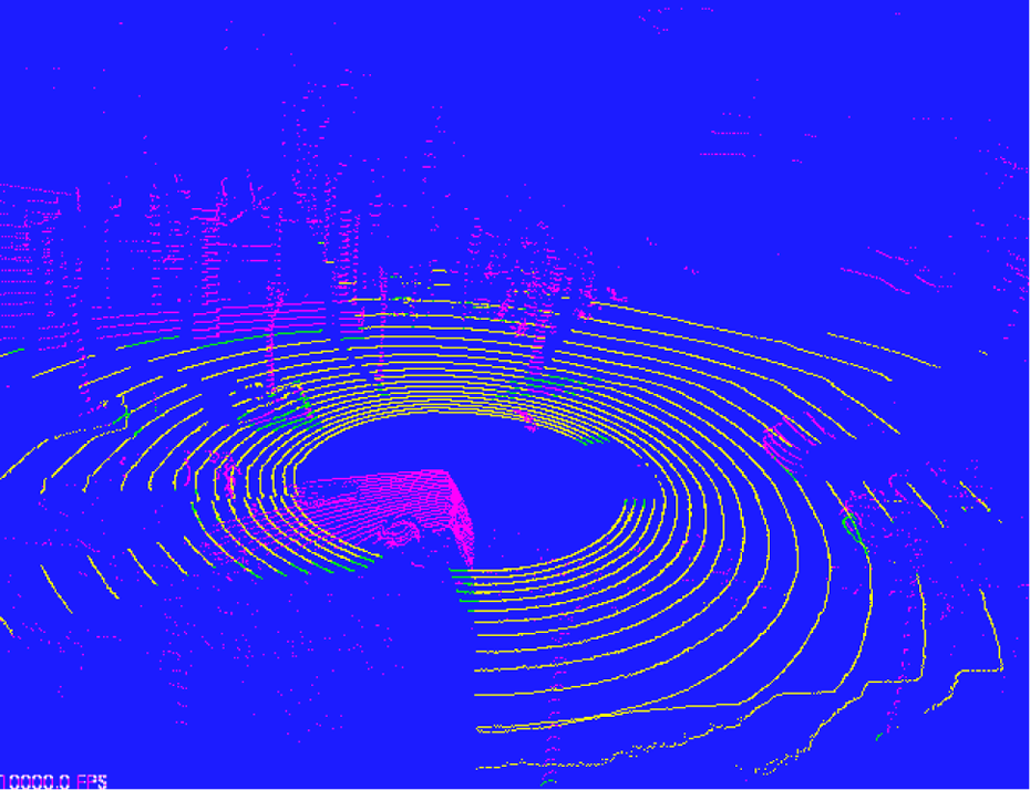
Figure 13 shows the result of using the naïve gradient threshold algorithm in good 3D point clouds. Figure 2 presents the meshes of a graph representation of this 3D view. The good 3D point clouds refer to the number of neighbors of each point in the cloud and the distance between them. According to the graph, nearly all vertices have four neighbors, and all edges have reasonable weights.

Figure 13.

Naïve gradient threshold on good data.

To achieve this result, we used maxgrad at 0.4 m, maxdh at 0.05, and mindistance at 0.4 m. In Figure 13, the yellow points represent the ground regions and the purple points represent other regions, such as non-ground regions. The ground region is almost visible near the position of the sensor that was segmented. Nevertheless, some other regions, such as points inside the green ellipse, had to be segmented as ground, which related to the under-segmented problem.

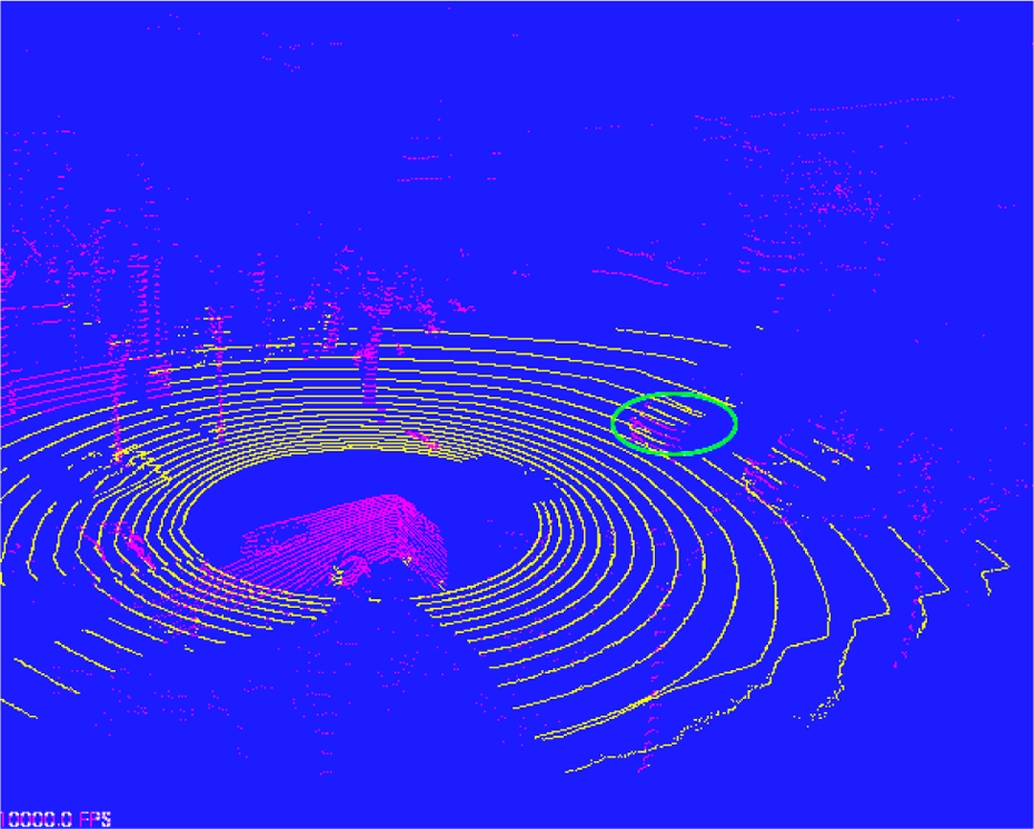
Figure 14 shows the result of our algorithm using the same data and the same threshold. However, we used other values for maxgrad, maxdh, and mindistance: 0.4, 0.05, and 0.4 m, respectively. In the figure, the white points denote non-ground regions. Green represents additional segmented points. The result is better than that of the naïve threshold technique.

Figure 14.

Our algorithm on good data.

In the case in which the threshold values increase, the result is over-segmented. We illustrate the result in Figure 15 when we use maxgrad as 0.6 m, maxdh as 0.05, and mindistance as 0.4 m. The points in the green eclipse are over-segmented. Nevertheless, it is not easy to properly choose threshold values.

Figure 15.

Over-segmented problem.

To more explicitly present our evaluation of the proposed ground segmentation method compared to the naïve gradient field approach, we provide screenshots of our experiments with two types of ground data. In Figures 16 and 17, the purple points represent non-ground regions, such as trees, walls, cars, or slope terrains that are impassable regions. The wrong points represent ground points that are traversable by the autonomous mobile robot which we already mentioned above about the under-segmented problem. These errors occurred in challenging regions where the gradient values were the same as the non-ground region near the boundaries or near the tree areas. These errors were accumulated over time on account of the algorithm working only frame by frame.

Figure 16.

Our algorithm with a flat, sparse terrain.

Figure 17.

Our algorithm with the slope, noisy terrain.

In Figure 16(a) and (b), the segmentation results of our algorithm by combining the naïve gradient field with the mean height evaluation produced a better result than that of using only the naïve gradient field with 82% segmentation of the flat, sparse terrain in our experiment. The segmentation result of the naïve gradient field is only 76%.

In Figure 17(a) and (b), we use the other data. The segmentation result of our algorithm is 76%, while the segmentation result of the naïve gradient field is 70%.

In our experiments, we apply the naïve gradient threshold technique with noisy data. In here, the naïve gradient threshold technique is a method for ground segmentation. This method is not about gradient evaluation. In our study, we still use the same technique for evaluating the gradient. However, for segmentation, we compare our technique with the technique that only naïve thresholding the gradient. The orders of some scanning lines are reversed with a maxgrad of 0.1 m, maxdh of 0.2 m, and mindistance of 10 m. The mesh of the graph representation of this 3D cloud data is given in Figure 3. The result is not good.

On the contrary, the segmentation result of our algorithm from the same data with the same threshold values produced a better result. To achieve this result, we applied two additional techniques that were given earlier with the uneven and sparse regions. Thus, the ground region was not 100% segmented, because we did not completely segment the ground points in each frame, such as at the further region of the center. The errors accumulated when we applied the algorithm on the accumulated 3D frame data.

Analysis

Figure 18 shows the processing time of our algorithm compared to the naïve gradient threshold, where the x-axis represents the number of mean points, and the y-axis represents the processing time in milliseconds. It can be seen that our algorithm is slightly slow but very efficient. This is because it requires time to analyze, preprocess the 3D cloud data, and handle it with the sparse and uneven regions. Nevertheless, this speed is not significant. In real-time processing, our algorithm achieved approximately 30 frames per second (fps).

Figure 18.

Time-consumption over the number of points.

Figure 19 illustrates the performance comparison of our algorithm and the naïve threshold technique. The x-axis represents the number of frames and the y-axis represents the processing time in milliseconds. The processing time was in 30 consecutive frames. When the number of frames increased, our algorithm was 15% slower than the naïve threshold technique.

Figure 19.

Processing time comparison in 30 frames.

Conclusions

In this article, we presented a new ground segmentation algorithm that combines three techniques: gradient threshold segmentation, adaptive break point detection, and neighbor mean height evaluation. The experimental results showed the proposed ground segmentation algorithm produced better results with two types of 3D data with different characteristics and uneven and sparse regions that could not be segmented using the gradient threshold technique.

We tested both algorithms with slope noisy and sparse data in real time. Our algorithm produced good results, as shown in Figure 17(a) and (b), and the performance was approximately 30 fps. Our method achieved good results in ground segmentation owing to the use of data preprocessing to remove noise, analysis of the structure to build a better representation graph, and managing the uneven and sparse regions.

Footnotes

Declaration of conflicting interests

The author(s) declared no potential conflicts of interest with respect to the research, authorship, and/or publication of this article.

Funding

The author(s) disclosed receipt of the following financial support for the research, authorship, and/or publication of this article: This work was supported by the National Research Foundation of Korea (NRF) grant funded by the Korea government (MSIP) (NRF-2015R1A2A2A01003779).

ORCID iD

Seoungjae Cho

References

Thrun

Montemerlo

Dahlkamp

. Stanley: the robot that won the DARPA grand challenge. J Field Robot (JFR) 2006; 23: 661–692.

Douillard

Underwood

Melkumyan

. Hybrid elevation maps: 3D surface models for segmentation. In: IEEE international conference on intelligent robots and system (IROS), Taipei, Taiwan, 18–22 October 2010, pp. 1532–1538. IEEE.

Pfaff

Triebel

Burgard

. An efficient extension to elevation maps for outdoor terrain mapping and loop closing. Int J Robot Res (IJRR) 2007; 26(2): 217–230.

Douillard

Underwood

Kuntz

. On the segmentation of 3D lidar point clouds. In: International conference on robotics and automation (ICRA 2011), Shanghai, China, 9–13 May 2011, pp. 2798–2805. IEEE.

Moosmann

Pink

Stiller

. Segmentation of 3D LIDAR data in non-flat urban environments using a local convexity criterion. In: IEEE intelligent vehicles symposium, Xi’an, China, 3–5 June 2009, pp. 215–220. IEEE.

Himmelsbach

Hundelshausen

Wuensche

Fast segmentation of 3d point clouds for ground vehicles. In: IEEE intelligent vehicles symposium (IV), San Diego, CA, USA, 21–24 June 2010, pp. 560–565. IEEE.

Lam

Kusevic

Mrstik

. Urban scene extraction from mobile ground based LIDAR data. In: 5th international symposium on 3D data, visualization & transmission, France, 17–20 May 2010, pp. 1–8.

Klasing

Wollherr

Buss

. A clustering method for efficient segmentation of 3d laser data. In: Robotics and automation, 2008. International conference on robotics and automation (ICRA) 2008. IEEE international conference, Pasadena, CA, USA, 19–23 May 2008, pp. 4043–4048. IEEE.

Friedman

Bentley

Finkel

. An algorithm for finding best matches in logarithmic expected time. ACM Trans Math Software 1977; 3(3): 209–226.

10.

Lari

Habib

Kwak

An adaptive approach for segmentation of 3D laser point cloud. In: ISPRS Workshop laser scanning 2011, Calgary, Canada, 29–31 August 2011, pp. 1–6.

11.

Chen

Dai

Liu

. 3D LIDAR-based ground segmentation. In: Asian conference on pattern recognition, Beijing, China, 28 November 2011, pp. 446–450. IEEE.

12.

Nguyen

Martinelli

Tomatis

. A comparison of line extraction algorithms using 2D laser rangefinder for indoor mobile robotics. In: International conference on intelligent robots and systems (IROS), Edmonton, Alta, 2–6 August 2005, pp. 1929–1934. IEEE.

13.

Nunez

Vazquez-Martin

Toro

. Feature extraction from laser scan data based on curvature estimation for mobile robotics. In: International conference on robotics and automation (ICRA), Orlando, FL, USA, 15–19 May 2006, pp. 1167–1172. IEEE.

14.

Jagannathan

Miller

. Three-dimensional surface mesh segmentation using curvedness-based region growing approach. IEEE Trans Pattern Anal Mach Intell 2007; 29(12): 2195–2204.

15.

Mokharian

Mackworth

. Scale-based description and recognition of planar curves and two-dimensional shapes. IEEE Trans Pattern Anal Mach Intell 1986; 8: 2–14.

16.

Montemerlo

Becker

Bhat

. Junior: the Stanford entry in the urban challenge. J Field Robot 2008; 25(9): 569–597.

17.

Thrun

. Learning occupancy grid maps with forward sensor models. Auton Robot 2003; 15(2): 111–127.

18.

Besl

Jain

. Segmentation through variable-order surface fitting. IEEE Trans Pattern Anal Mach Intell 1988; 10(2): 167–192.

19.

Hoover

Jean-Baptiste

Jiang

. An experimental comparison of range image segmentation algorithms. IEEE Trans Pattern Anal Mach Intell 1996; 18(7): 673–689.

20.

Fischler

Bolles

. Random sample consensus: a paradigm for model fitting with applications to image analysis and automated cartography. Communications of the ACM 1981; 24: 381–395.

21.

Strom

Richardson

Olson

. Graph-based segmentation for colored 3D laser point clouds. In: IEEE/RSJ international conference on intelligent robots and systems (IROS), Taipei, Taiwan, 18–22 October 2010, pp. 1532–1538. IEEE.

22.