Mobile robot wall-following control using a fuzzy cerebellar model articulation controller with group-based strategy bacterial foraging optimization

Abstract

In this study, a fuzzy cerebellar model articulation controller based on group-based strategy bacterial foraging optimization is proposed for mobile robot wall-following control. In fuzzy cerebellar model articulation controller, the inputs are the distance between the sonar and the wall, and the outputs are the angular velocity of two wheels. The proposed group-based strategy bacterial foraging optimization learning algorithm is used to adjust the parameters of fuzzy cerebellar model articulation controller model. The proposed group-based strategy bacterial foraging optimization has the advantages of global search, evolutionary strategies, and group evolution to speed up the convergent rate. A new fitness function is defined to evaluate the performance of mobile robot wall-following control. The fitness function includes four assessment factors which are defined as follows: (1) maintaining safe distance between the mobile robot and the wall, (2) ensuring successfully running a cycle, (3) avoiding mobile robot collisions, and (4) mobile robot running at a maximum speed. The experimental results show that the proposed group-based strategy bacterial foraging optimization obtains a better wall-following control than other methods in unknown environments.

Introduction

In recent years, mobile robot control is one of the popular research areas, which includes wall-following control, navigation, parallel parking and path tracking, and so on. The wall-following control is the fundamental requirement for navigation and parallel parking, and its purpose is to enable the robot to explore in unknown environments. Therefore, this study focuses on mobile robot wall-following control.

In general, because external noise interference and sensitivity of sensing module exist, traditional control methods are difficult to control the stable behavior of robot. In order to solve the design problem of controller, fuzzy logic control has been successfully applied on the robot control problem. ^{1 –3} Fuzzy logic ⁴ was proposed by Zadeh in 1965, which can be used to deal with imprecise, ambiguous, and uncertainty problems. A fuzzy controller consists of four parts: fuzzification, rule base, fuzzy inference engine, and defuzzification.

Neural networks and fuzzy theory ^{5 –9} have been used successfully in various fields. In neural networks, both the multilayer neural network and the cerebellar model articulation controller (CMAC) ⁷ are widely adopted. The CMAC model imitates the human cerebellar cortex, and the input space of its structure is quantized to discrete state referred to hypercube. The excited hypercubes are used to map the different states of the storage allocation information in memory cells. Finally, retrieve the corresponding information from the memory cell and output the results by accumulating operation. The advantages of CMAC are fast convergence speed and easy hardware implementation. However, there are still some shortcomings in CMAC, such as larger required computing memory, the advantage of mapping by performing local approximation of the hyperplanes is not fully exploited, and difficulty of adaptively selecting structural parameters. Therefore, many modified CMAC models ^8,9 were proposed to resolve these shortcomings, such as hierarchical cerebellar model articulation controller ⁸ and fuzzy cerebellar model articulation controller (FCMAC). ⁹

The related parameters of CMAC model are usually adjusted by backpropagation (BP) algorithm. The BP algorithm is based on a fast gradient descent, which is used to adjust the parameters of CMAC model by the error function. The BP algorithm has a fast convergence speed. Thus, it is usually used to solve several engineering problems. However, the BP algorithm has the disadvantage of falling into the local minimum. Therefore, many researchers ^{10 –15} adopted the evolutionary computation methods to obtain the global optimum. These algorithms derive from observing the phenomenon of the natural world and the imitation of various biological behaviors, such as predatory strategy, social organization, evolution, and so on. First, genetic algorithms ^10,11 were based on Darwin’s theory of evolution and Mendelian inheritance. The method is essentially a kind of high efficiency, parallel processing, and global search algorithms. In other words, in order to achieve the optimal solution, this method can automatically acquire and accumulate knowledge on searching space during a search processing and adaptively control the reaching process. Secondly, several researchers have proposed different evolutionary computation algorithms, such as ant colony optimization, ¹² particle swarm optimization, ¹³ differential evolution, ¹⁴ and bacterial foraging optimization (BFO). ¹⁵

Recently, BFO has been applied in various fields successfully, ^{16 –18} such as model predictive control, adaptive estimation, portfolio optimal and classification, and so on. The traditional BFO has several advantages, such as less parameters, good robustness, parallel processing, and global search ability. Poor accuracy and slow convergence speed happen in traditional BFO when solving more complex problems; especially on dealing with the multi-peak problems. Therefore, a modified BFO is proposed to improve the traditional BFO.

In this study, the fuzzy theory will be embedded into the traditional CMAC model. In order to solve more hypercube cells required in the traditional CMAC, the inputs use Gaussian membership function and form a fuzzy hypercube, and a linear combination of input variables in the consequent memory is used to replace a single value memory. Therefore, an FCMAC model is proposed for mobile robot wall-following control. In addition, to avoid the drawbacks of poor accuracy, slow convergence speed, and the multi-peak problem in traditional BFO, this study proposes a group-based strategy bacterial foraging optimization (GSBFO) to adjust the parameters of FCMAC model. The proposed GSBFO has the advantages of global search, evolutionary strategies, and group evolution to speed up the convergent rate. Thus, the algorithm can efficiently obtain the global optimal solution. Experimental results show that the proposed FCMAC with GSBFO can successfully implement mobile robot wall-following control and has a better performance than other methods.

The rest of this article is organized as follows: “Description of mobile robot” section describes the mobile robot of Pioneer 3-DX. “An improved bacterial foraging optimization of FCMAC model” section presents the proposed FCMAC with GSBFO. The experimental results of several unknown environments are described in “Experimental results” section. The final section draws the conclusions.

Description of mobile robot

The mobile robot of Pioneer 3-DX is introduced by US MobileRobots. ¹⁹ The characteristics of the mobile robot are high payload, high endurance, strong extensibility, and support cross-platform software development kit (SDK). This SDK includes motion control, client–server architecture, and various accessories. Therefore, users can apply the robot to various fields and integrate all peripheral equipment to complete the research goals.

In Figure 1, the Pioneer 3-DX mobile robot consists of three wheels, where two wheels are used to drive the mobile robot and one auxiliary wheel is used to keep the stabilization of a mobile robot. The positions of sonar arrays in Pioneer 3-DX robot are fixed: one on each side and six facing outward at 20° intervals. Sensitivity ranges from 10 cm (6 inches) to 5 m. It is a fully autonomous intelligent mobile robot. Table 1 shows the Pioneer 3-DX specification.

Figure 1.

Pioneer 3-DX.

Table 1.

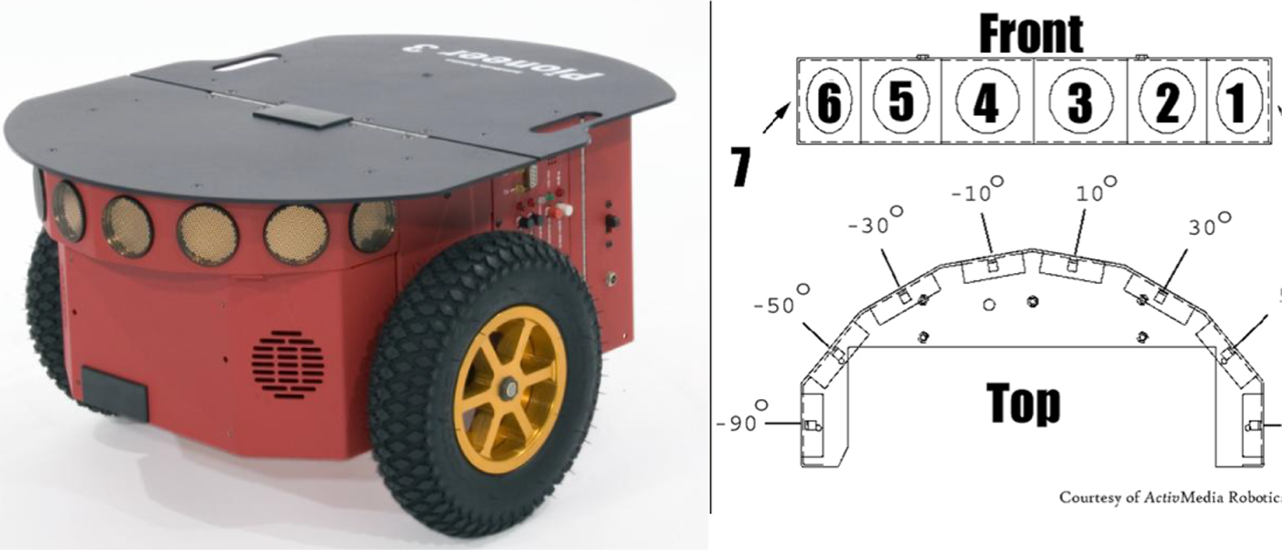
Pioneer 3-DX specification.

Length/width/height (cm)	44/39/23
Weight (kg)	9
Translate speed max (mm/s)	1400
Wheels diameter/width (mm)	195/47

An improved BFO of FCMAC model

In this session, the structure of proposed FCMAC model will be introduced in subsection “A fuzzy cerebellar model articulation controller”. “The proposed GSBFO” subsection describes an improved bacteria foraging optimization algorithm, which is called GSBFO. The proposed learning algorithm is used to adjust the parameters of FCMAC model for implementing mobile robot wall-following control.

A fuzzy cerebellar model articulation controller

The traditional CMAC model adopts the concept of multi-hypercube and memory cells and the mapping technique to store the information of the different states in the corresponding multi-hypercube cells. Finally, access the information from the corresponding memory cells and accumulate it as output. In this study, the fuzzy theory will be embedded into the traditional CMAC model. The inputs use Gaussian membership function and form a fuzzy hypercube. A linear combination of input variables in the consequent memory is used to replace a single value memory. In order to solve more hypercube cells required in the traditional CMAC, this study proposes a FCMAC model and its structure is shown in Figure 2.

Figure 2.

The structure of FCMAC model. FCMAC: fuzzy cerebellar model articulation controller.

In each node, $u_i^{\left(l\right)}$ and $o_i^{\left(l\right)}$ represent the lth layer network and the ith input and output. These layers sequentially are described as follows:

(1) Layer 1 (input layer)

Input variables $X=\left\{x_1,\dots ,x_n\right\}$ are directly into network. Only transfer messages and no function calculation exist

$o_i^{\left(1\right)}=u_i^{\left(1\right)},\text{ and }{u}_i^{\left(1\right)}=x_i$

1

• (2) Layer 2 (fuzzification layer)

The fuzzification layer is to fuzzify the output of layer 1 and each node uses Gaussian membership function to perform fuzzification operation. It is defined as follows

$o_i^{\left(2\right)}=\text{ exp}\left(-\frac{{\left[u_i^{\left(2\right)}-m_{ij}\right]}^2}{{\mathit{\sigma }}_{ij}{ }^2}\right),\text{ and }{u}_i^{\left(2\right)}=o_i^{\left(1\right)}$

2

where $m_{ij}\text{ and }{\mathit{\sigma }}_{ij}$ represent the jth center and width of Gaussian membership function in the ith input dimension, respectively.

• (3) Layer 3 (spatial firing layer)

Each node represents the fuzzy hypercube cells by assembling the output of layer 2. This node performs fuzzy product operator to obtain the firing strength α_j in space. The output is calculated as follows

${o_j}^{\left(3\right)}={\alpha }_j={\displaystyle \prod }_i{u_{ij}}^{\left(3\right)},\text{ and }{u_{ij}}^{\left(3\right)}={o_{ij}}^{\left(2\right)}$

3

where $\prod _i{u_{ij}}^{\left(3\right)}$ represents the firing strength of the corresponding fuzzy hypercube cells.

• (4) Layer 4 (consequent layer)

Each node represents one memory. The information from internal memory is a linear combination of input variables. The firing strength α_j maps to the corresponding memory for obtaining a fuzzy output. It is expressed as follows

${o_j}^{\left(4\right)}={u_j}^{\left(4\right)}\left(a_{0j}+{\displaystyle \sum }_{i=1}^D{a}_{ij}{x}_i\right),\text{ and }{u_j}^{\left(4\right)}={o_j}^{\left(3\right)}$

4

where $a_{0j}\text{ and} a_{ij}$ represent constants and D indicates the input dimension.

• (5) Layer 5 (output layer)

The final output y adopts centroid of area to perform defuzzification

$y=\frac{{{\displaystyle \sum }}_{j=1}^R{o}^{\left(4\right)}}{{{\displaystyle \sum }}_{j=1}^R{o}^{\left(3\right)}}$

5

where R is the number of fuzzy hypercube cells.

The proposed GSBFO

In this section, the proposed GSBFO will be introduced. The proposed learning method can be effectively used to adjust the parameters of FCMAC model.

The encoding of one bacterium in FCMAC is shown in Figure 3. One fuzzy hypercube cell contains the center m_ij and width σ_ij of Gaussian membership function and the constants a_0j and a_ij of the corresponding memory of linear combination of input variables.

Figure 3.

Encoding of one bacterium in FCMAC. FCMAC: fuzzy cerebellar model articulation controller.

The traditional BFO was proposed by Passino. ¹⁵ Bacteria searches the better quality solution via chemotaxis, reproduction, and elimination-dispersal. In the chemotaxis operation, bacteria uses tumble and swim to move to their location. Therefore, bacteria usually search randomly in various regions, and this operation can increase the diversity of searching range. On the contrary, it may ignore the searching capabilities of the better range.

In order to overcome the aforementioned problems, this study proposes an efficient GSBFO algorithm. The flowchart of GSBFO is shown in Figure 4. In GSBFO, the evolutionary strategy of chemotaxis operation process is used. Thus, bacteria in the chemotaxis process have the opportunity to move to the best location $P_{l\text{best}}^i$ of own, the best location $B_{\text{leader}}^j$ of a group, and the best location $P_{g\text{best}}^{ }$ of a swarm. In addition, in order to improve the searching capability of optimal area, a group concept ^20,21 is introduced. Before the chemotaxis operation process is executed, the fitness functions of a swarm are arrayed in ascending order. Then, we use the concept of “Birds of a feather flock together.” That is, the similar bacteria will form the same bacteria group. The detailed group formation process is shown in Figure 5.

Figure 4.

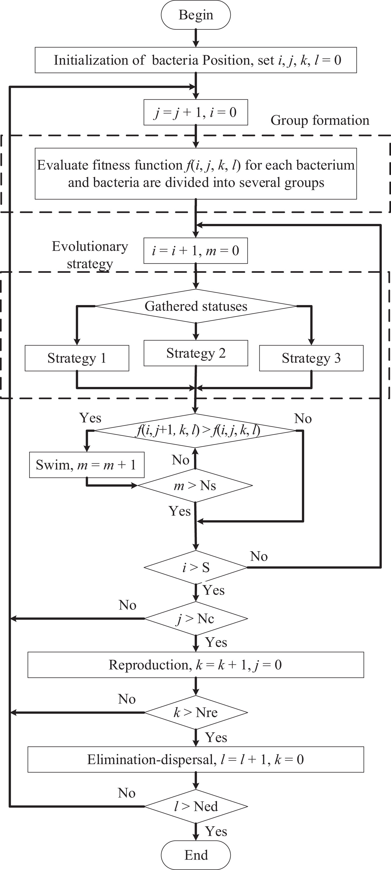
The flowchart of GSBFO. GSBFO: group-based strategy bacterial foraging optimization.

Figure 5.

Group formation process.

• (1) Group formation

Step 1: The fitness functions of a swarm are arrayed in ascending order.

Step 2: Find the threshold τ_th of group formation. The maximum fitness value P_best and the minimum fitness value P_worst in a swarm are selected. According to the locations of two bacteria (P_best and P_worst), we can calculate the threshold of group formation. The formula is shown as follows

${\tau }_{\text{th}}=d\times \sqrt{\frac{{{\displaystyle \sum }}_{i=1}^n{\left(P_{\text{best}}^{ }\left(i\right)-P_{\text{worst}}^{ }\left(i\right)\right)}^2}{n}}$

6

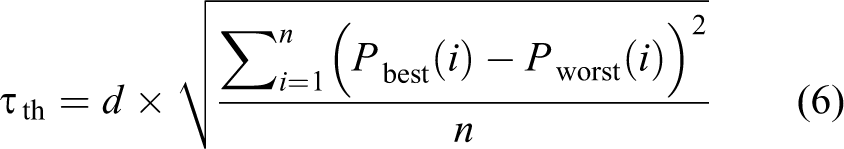
where n is the size of bacterial cell structure and d is a constant between 0 and 1. In general, d is usually set to 0.6.

Step 3: First, set a bacterium with the maximum fitness value P_best in a swarm as the leader of local best position in the group 1 $\left(G1\right) B_{\text{leader}}^1$ . Then, use $B_{\text{leader}}^1$ to compare similarity with other bacteria in the swarm sequentially. If the similarity is smaller than the threshold τ_th, the bacteria will be classified as G1. After the G1 is completed, then find the maximum fitness value from the remaining bacteria with unfinished group in the swarm as the leader of local best position in the group 2 (G2) $B_{\text{leader}}^2.$ Then, use $B_{\text{leader}}^2$ to compare similarity with the remaining bacteria with unfinished group in the swarm sequentially. If the similarity is smaller than the threshold τ_th, the bacteria will be classified as G2, and so on.

• (2) Evolutionary strategy

In the proposed GSBFO, the states of the previous two bacterial chemotactic processes will be recorded. The states consist of deterioration, status quo, and improvement. Therefore, there are nine gathered-statuses based on the previous two bacterial chemotactic operations. According to the nine gathered-statuses, three strategies are generated and shown in Table 2. These strategies are applied in the tumble step of the bacterial chemotactic process.

Table 2.

The gathered-statuses and evolutionary strategies of bacteria.

Gathered-statuses	Evolutionary strategies
(=,+)(+,+)	Strategy 1
(−,+)(+,=)	Strategy 2
(−,−)(=,−)(+,−)(−,+)(=,=)	Strategy 3

Deterioration: −; status quo: =; improvement: +.

• Strategy 1: In this strategy, the moving of bacteria will tend to the global best bacterium in the swarm ( $P_{g\text{best}})$ and the leader in the jth group $\left( B_{\text{leader}}^j\right)$ . This strategy can efficiently narrow the search range and accelerate the convergent speed

${\mathit{\theta }}^i=0.3\times \text{CS}+w_1\times C\left(i\right)\times \left(P_{g\text{best}}-{\mathit{\theta }}^i\right)+w_2\times C\left(i\right)\times \left(B_{\text{leader}}^j-{\mathit{\theta }}^i\right)$

7

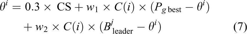
where CS is the movement step of the last chemotactic operation, C(i) is the size of the step taken in the random direction as specified in the tumble step, $P_{g\text{best}}$ denotes the global best bacterium in the swarm, θⁱ presents the ith bacterium position, and $B_{\text{leader}}^j$ is the leader in jth group.

$\begin{array}{l}{w}_1=K\times \frac{f\left(P_{g\text{best}}\right)}{f\left(P_{g\text{best}}\right)+f\left(B_{\text{leader}}^j\right)},\\ w_2=K\times \frac{f\left(B_{\text{leader}}^i\right)}{f\left(P_{g\text{best}}\right)+f\left(B_{\text{leader}}^j\right)}\end{array}$

where the step coefficient K is set to [4, 6] and f(⋅) indicates the fitness function.

Strategy 2: In this strategy, the moving of bacteria will tend to the local best position $\left(P_{l\text{best}}^i\right)$ and the leader in the jth group $\left(B_{\text{leader}}^j\right)$ . This strategy can enhance the local search ability

${\mathit{\theta }}^i=0.9\times \text{CS}+w_1\times C\left(i\right)\times \left(P_{l\text{best}}^i-{\mathit{\theta }}^i\right)+w_2\times C\left(i\right)\times \left(B_{\text{leader}}^j-{\mathit{\theta }}_{ }^i\right)$

8

where $w_1=K\times \frac{f\left(P_{l\text{best}}^i\right)}{f\left(P_{l\text{best}}^i\right)+f\left(B_{\text{leader}}^j\right)},w_2=K\times \frac{f\left(B_{\text{leader}}^j\right)}{f\left(P_{l\text{best}}^i\right)+f\left(B_{\text{leader}}^j\right)}$

The step coefficient K is set the same as strategy 1.

Strategy 3: This is a random search strategy. It can be used to expand the diversity of the search range

${\mathit{\theta }}^i=C\left(i\right)\times \frac{\Delta \left(i\right)}{\sqrt{{\Delta }^T\left(i\right)\times \Delta \left(i\right)}}$

9

where Δ(i) is a random direction and its value is set as [−1, 1].

Experimental results

In order to verify the performance of proposed GSBFO, we will apply the mobile robot wall-fallowing control problem and compare the proposed method with various methods. The experiment consists of the simulated control and the practical control of mobile robot. In the simulation experiment, the Webots PRO 7.4.3 simulator software (https://www.cyberbotics.com/) is used to simulate the Pioneer 3-DX mobile robot.

The environment of mobile robot is shown in Figure 6. The mobile robot has three input signals, such as the distance S1 from 10° angle sonar, the distance S2 from 50° angle sonar, and the distance S3 from 90° angle sonar. The detecting distance of sonar sensors is limited between 0.1 and 5 m. The two output signals control the velocity of left wheel (V _L) and the velocity of right wheel (V _R) of mobile robot. The outputs are limited in the interval [−5.24, 5.24] (rad/s). The execution cycle of mobile robot is 500 ms. Figure 7 shows the control diagram of the mobile robot using an FCMAC controller with GSBFO learning algorithm.

Figure 6.

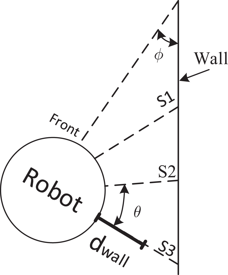
Environment of mobile robot.

Figure 7.

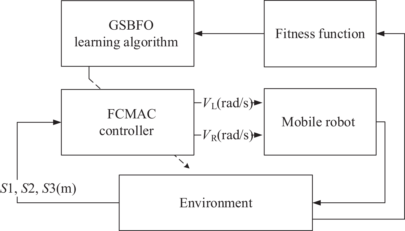
The mobile robot control using an FCMAC controller. FCMAC: fuzzy cerebellar model articulation controller.

In the experimental process, the mobile robot wall-fallowing control includes three terminal conditions. In evolutionary process, when the terminal conditions occur, the number of evolution will be added one, and the robot returns to the initial position of the experiment and reperforms again. The evolutionary process will be terminated until the mobile robot detours around the venue of an unknown environment successfully. Three terminal conditions are described as follows:

Mobile robot collides with the wall. For example, the distance from the sonar sensor is less than 0.1 m.

The robot is far away from the wall. For example, the distance S3 is greater than 0.7 m.

The mobile robot can detour around the venue successfully.

Table 3 shows the initial parameters set of proposed algorithm. The objective function of a controller depends on the environment of mobile robot. In this study, the assessment factors consist of four objective functions ${\text{CF}}_{\text{1}}\text{,}\hspace{0.17em}{\text{CF}}_{\text{2}}\text{,}\hspace{0.17em}{\text{CF}}_{\text{3}}{\text{, and CF}}_{\text{4}}$ , and are defined as follows:

Table 3.

Initial parameters setting of the proposed algorithm.

Number of fuzzy hypercube	S	Ned	Nre	Nc
3	50	2	5	100
Ns	Ped	C(i)	d	k
4	0.25	0.1	0.6	5

• (1) Objective function CF₁: When a collision occurs, the proportionality of the robot moving distance (T_dis) and the predefined walking with maximum distance (T_stop) is defined as follows

${\text{CF}}_1=1-\frac{T_{\text{dis}}}{T_{\text{stop}}}$

10

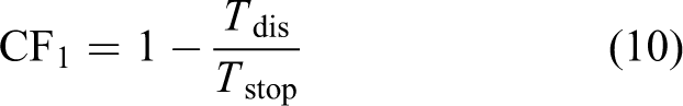
• If the actual moving distance of mobile robot is larger than the walking with maximum distance (T_stop), we set $T_{\text{dis}}=T_{\text{stop}}$ . In this situation, the robot has satisfied the objective function CF₁. If the collision-free control occurs, the value of objective function CF₁ is set to zero.

• (2) Objective function CF₂: The objective function describes the distance (RD(t)) between the right wheel of mobile robot and the wall at time step t. If the mobile robot moves the wall-following with the desired path, the RD(t) will be zero at time step t. RD(t) is defined as follows

$\text{RD}\left(t\right)=\left|S3\left(t\right)-d_{\text{wall}}\right|$

11

• where d_wall is the predefined wall-robot distance to be maintained. The goal of CF₂ is defined as the average value of RD(t) at all time steps T_total

${\text{CF}}_2=\frac{{{\displaystyle \sum }}_{t=1}^{T_{\text{total}}}\text{RD}\left(t\right)}{T_{\text{total}}}$

12

• (3) Objective function CF₃: The objective function describes the angle (∅) between the front of mobile robot and the wall, as shown in Figure 6. If the mobile robot moves parallel to the wall, then the angle ∅ is zero. The angle ∅(t) is defined as follows

$\varnothing \left(t\right)=\left|{\text{tan}}^{-1}\left(\frac{S1-S2\text{cos}\mathit{\theta }}{S2\text{sin}\mathit{\theta }}\right)\right|$

13

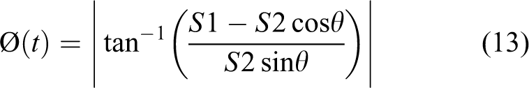
• where θ is an angle between S2 and S3 of sonar sensing distances. The CF₃ is the average angle ∅(t) at all time steps T_total defined as follows

${\text{CF}}_3=\frac{{{\displaystyle \sum }}_{t=1}^{T_{\text{total}}}\mathit{\varnothing }\left(t\right)}{T_{\text{total}}}$

14

• (4) Objective function CF₄: The objective function describes the proportionality between an average moving speed (V_average) of mobile robot and the predefined desired speed (V_hope)

${\text{CF}}_4=1-\frac{V_{\text{average}}}{V_{\text{hope}}}$

15

If the average moving speed is greater than the predefined desired speed, we set V_average = V_hope. This indicates that the mobile robot has satisfied the conditions. The goal of CF₄ is to move the mobile robot at high speed.

The fitness function f(⋅) is based on the control factor of four objective functions CF₁, CF₂, CF₃, and CF₄, which combines the weighting coefficients α₁, α₂, α₃, and α₄ to form a total objective function

$f(\cdot )=\frac{1}{1+\left({\alpha }_1{\text{CF}}_1+{\alpha }_2{\text{CF}}_2+{\alpha }_3{\text{CF}}_3+{\alpha }_4{\text{CF}}_4\right)}$

16

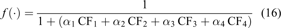
In equation (16), we can find that the goal of the fitness function f(·) converges approaching to 1. In addition, the sum of the weighting coefficients is equal to 1. In this study, the weighting coefficients of control factors are set as $[{\alpha }_1,{\alpha }_2,{\alpha }_3,{\alpha }_4\left]=\right[0.45,0.45,0.05,0.05]$ . In order to avoid a behavior of collision control and keep a fixed distance between the robot and the wall, the two objective functions CF₁ and CF₂ are very important. Therefore, the weighting coefficients α₁ and α₂ are set to 0.45, whereas the remaining weighting coefficients α₃ and α₄ are set to 0.05.

Training of environment

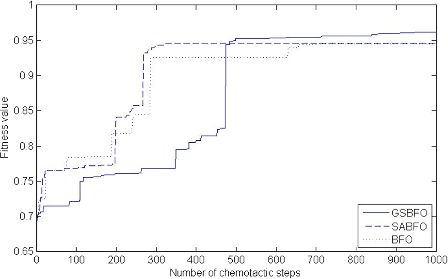
Firstly, the training environment is set to 5 × 4 m, as shown in Figure 9. It consists of the straight line, the bevel angle, and the right angle problems. The starting point of mobile robot is (x, y) = (2, −1.5). The distance from the start point to the target point is 18 m, d_wall is set to 0.3 m, and V_hope is set to 0.4 m/s. This study compares the proposed GSBFO algorithm to the BFO algorithm ¹⁵ , and the Strategy-Adaptation-based Bacterial Foraging Optimization (SABFO) algorithm. ¹⁸ Each of these algorithms is applied to the mobile robot wall-following control. The performance measures include the best fitness function, the worst fitness function, the average fitness function, and the standard deviation. Figure 8 illustrates the obtained fitness functions by different learning algorithms. The best fitness functions by the proposed GSBFO, the SABFO, ¹⁸ and the BFO ¹⁵ learning methods are 0.962, 0.945, and 0.944, respectively. The comparison results are shown in Table 4. The proposed GSBFO has better fitness function than other methods, ^15,18 under the same conditions. In Table 4, the proposed GSBFO has the smallest standard deviation than other methods. ^15,18 Therefore, the proposed GSBFO method is more stable than other methods.

Figure 8.

The best fitness function by different learning algorithms.

Figure 9.

The moving path of mobile robot using the proposed algorithm in training environment.

Table 4.

Comparison results of the best fitness function, the worst fitness function, the average fitness function, and standard deviation.

	Best	Worst	Average	Standard deviation
GSBFO	0.962	0.946	0.954	0.005
SABFO 18	0.945	0.856	0.923	0.034
BFO 15	0.944	0.795	0.908	0.056

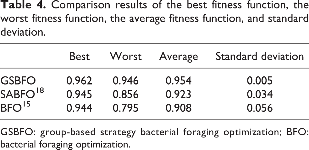
GSBFO: group-based strategy bacterial foraging optimization; BFO: bacterial foraging optimization.

The learned FCMAC model is applied to simulate the robot wall-following control. Figure 9 presents the moving path of mobile robot by the proposed FCMAC model with GSBFO learning algorithm. In this figure, the proposed algorithm gives a good wall-following control in points A and B of a bevel angle, and points C and D of a right angle control problems. In addition, the root-mean-square error (RMSE) is effectively used to evaluate the control factor CF₂ of the mobile robot wall-following control problem. The mobile robot maintains a fixed distance from the wall and the RMSE is defined as follows

$\text{RMSE}=\sqrt{\frac{{{\displaystyle \sum }}_{t=1}^{T_{\text{total}}}{\left(S3\left(t\right)-d_{\text{wall}}\right)}^2}{T_{\text{total}}}}$

17

The simulation results are shown in the second row of Table 5. The RMSE results of the training environment using the proposed GSBFO, the SABFO, and the BFO methods are 0.032, 0.052, and 0.069, respectively. Experimental results show that the proposed GSBFO method has a smaller RMSE than other methods. ^15,18

Table 5.

Comparison results of RMSE using various learning algorithms.

Algorithms\Environments	GSBFO	SABFO 18	BFO 15
Training environment	0.032	0.052	0.069
Testing environment 1
Without disturbance	0.043	0.056	0.078
With disturbance	0.088	—	0.098
Testing environment 2
Without disturbance	0.044	0.054	—
With disturbance	0.054	0.067	—

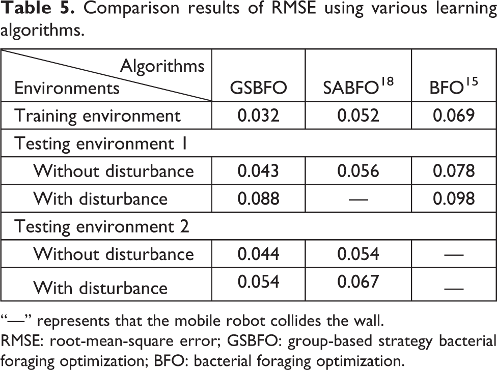
“—” represents that the mobile robot collides the wall.

RMSE: root-mean-square error; GSBFO: group-based strategy bacterial foraging optimization; BFO: bacterial foraging optimization.

In order to verify the robust ability of the proposed algorithm, two complex and noise interference environments are adopted in this study. Finally, experimental verification mobile robot can be successfully implemented with the wall-following control in an unknown environment.

Testing environment 1

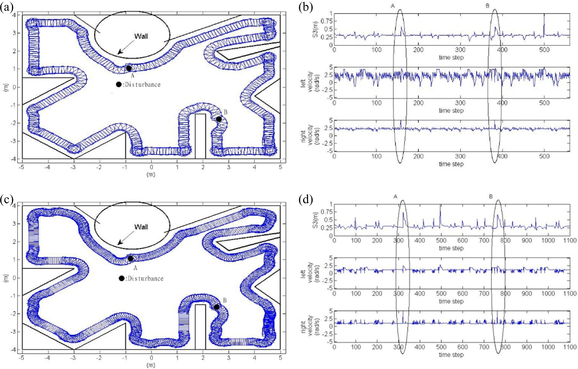
Testing environment 1 is set to 10 × 8 m. The distance from the start point to the target point is 65 m. In a continuously changing environment, some different learning methods are used for implementing the mobile robot wall-following control. Figure 10(a), (c), and (e) shows the moving path of the mobile robot in testing environment 1 using the proposed GSBFO, the SABFO, ¹⁷ and the BFO ¹⁵ methods. Figure 10(b), (d), and (f) indicates the robot sonar sensing distance to the wall and the wheel speed at each time step. The RMSE results in testing environment 1 using the proposed GSBFO, the SABFO, and the BFO methods are 0.043, 0.056, and 0.078, respectively. The RMSE results without disturbance are shown in the third row of Table 5. In addition, we have added a disturbance to verify the robust capability for various learning algorithms. During the testing process, we add a disturbance signal to the two-wheel outputs. That is, at points A and B, we added disturbance signals of 5.24 rad/s and 0 rad/s, respectively, to the two-wheel outputs V _R and V _L. Figure 11(a), (c), and (e) presents the moving trajectory of mobile robot with disturbance in testing environment 1, whereas Figure 11(b), (d), and (f) indicate the robot sonar sensing distance to the wall and the wheel speed at each time step. In testing environment 1, disturbance is added at points A and B. Figure 11(c) shows the SABFO algorithm ¹⁸ collides with the corner after adding a disturbance at point B, which is indicated by the symbol “^ ”. The RMSE results in testing environment 1 using the proposed GSBFO, the SABFO, and the BFO methods are 0.088, —, and 0.098, respectively. The symbol “—” indicates that the robot collides with the wall. The RMSE results with disturbance are also shown in the fourth row of Table 5. The simulation results also show that the proposed method gives a smaller RMSE and has a better robust ability than other algorithms, ^15,17

Figure 10.

The simulation results without disturbance in testing environment 1. The moving trajectory of mobile robot using (a) GSBFO, (c) SABFO, ¹⁸ (e) BFO ¹⁵ and the sonar sensing distance and the angular velocity of two wheels using (b) GSBFO, (d) SABFO, ¹⁸ (f) BFO. ¹⁵ GSBFO: group-based strategy bacterial foraging optimization; BFO: bacterial foraging optimization.

Figure 11.

The simulation results with disturbance in testing environment 1. The moving trajectory of mobile robot using (a) GSBFO, (c) SABFO, ¹⁷ (e) BFO ¹⁵ and the sonar sensing distance and the angular velocity of two wheels in (b) GSBFO, (d) SABFO, ¹⁸ (f) BFO. ¹⁵ GSBFO: group-based strategy bacterial foraging optimization; BFO: bacterial foraging optimization.

Testing environment 2

The setting conditions of testing environment 2 are the same as testing environment 1. Figure 12(a), (c), and (e) presents the moving trajectory of mobile robot in testing environment 2, which has no influence of disturbance. Figure 12(b), (d), and (f) indicates the robot sonar sensing distance and the wheel speed at each time step. In testing environment 2, Figure 12(e) illustrates that the robot collides with the wall using the BFO learning algorithm. ¹⁵ The RMSE results without disturbance in testing environment 2 using the proposed GSBFO, the SABFO, and the BFO methods are 0.044, 0.054, and —, respectively. The RMSE results without disturbance are shown in the fifth row of Table 5. In addition, disturbance signals at points A and B are also added in testing environment 2. Figure 12(e) illustrates that the mobile robot collides with the wall using the BFO method. ¹⁵ Therefore, Figure 13 only shows the simulation results with disturbance by the proposed GSBFO and the SABFO methods. In this figure, the proposed method quickly keeps a fixed distance from the wall when the mobile robot encounters a disturbance. The RMSE results with disturbance in testing environment 2 using the proposed GSBFO, the SABFO, and the BFO methods are 0.054, 0.067, and —, respectively. The RMSE results with disturbance are shown in the sixth row of Table 5. In this table, we can find that simulation results show the proposed GSBFO method has better robust ability than other methods, ^15,18 when the mobile robot encounters a disturbance.

Figure 12.

The simulation results without disturbance in testing environment 2. The moving trajectory of mobile robot using (a) GSBFO, (c) SABFO, (e) BFO and the sonar sensing distance and the angular velocity of two wheels in (b) GSBFO, (d) SABFO, (f) BFO. GSBFO: group-based strategy bacterial foraging optimization; BFO: bacterial foraging optimization.

Figure 13.

The simulation results with disturbance in testing environment 2. The moving trajectory of mobile robot using (a) GSBFO, (c) SABFO and the sonar sensing distance and the angular velocity of two wheels in (b) GSBFO, (d) SABFO. GSBFO: group-based strategy bacterial foraging optimization.

Testing real environment

Finally, the proposed GSBFO algorithm is used to control the Pioneer 3-DX mobile robot in a real environment. Since the real environment has the uncertainty and unpredictability characteristics, the control of a real mobile robot is difficult. The real testing environment is set as the range of size 4 × 2.5 m, as shown in Figure 14. Experimental results demonstrate the proposed algorithm can successfully implement the mobile robot wall-following control in a real unknown environment.

Figure 14.

The wall-following control using the proposed GSBFO algorithm in real environment. GSBFO: group-based strategy bacterial foraging optimization.

Conclusion

This study proposes the mobile robot wall-following control using an FCMAC with GSBFO learning method. The proposed GSBFO has the advantages of global search, evolutionary strategies, and group evolution to speed up the convergence rate. Thus, the proposed method is not easy to fall into the regional solution. Two simulated testing environments without/with disturbance and a real environment are used to validate the effectiveness of the proposed GSBFO algorithm. Experimental results show that the proposed method in the testing environments without/with disturbance are better than the traditional BFO ¹⁵ and the SABFO ¹⁸ algorithms.