Sage Journals: Discover world-class research

Abstract

Positive obstacles will cause damage to field robotics during traveling in field. Field autonomous land vehicle is a typical field robotic. This article presents a feature matching and fusion-based algorithm to detect obstacles using LiDARs for field autonomous land vehicles. There are three main contributions: (1) A novel setup method of compact LiDAR is introduced. This method improved the LiDAR data density and reduced the blind region of the LiDAR sensor. (2) A mathematical model is deduced under this new setup method. The ideal scan line is generated by using the deduced mathematical model. (3) Based on the proposed mathematical model, a feature matching and fusion (FMAF)-based algorithm is presented in this article, which is employed to detect obstacles. Experimental results show that the performance of the proposed algorithm is robust and stable, and the computing time is reduced by an order of two magnitudes by comparing with other exited algorithms. This algorithm has been perfectly applied to our autonomous land vehicle, which has won the champion in the challenge of Chinese “Overcome Danger 2014” ground unmanned vehicle.

Keywords

3-D LiDAR field ALV positive obstacle detection FMF algorithm

Introduction

A field autonomous land vehicle (ALV) is a typical field robot that drives off-road. In order to keep itself safe, the vehicle needs to detect both positive and negative obstacles by its own sensors.¹ In the past decades, many literatures have emerged to address the problem of obstacle detection.^2,3 But heretofore, ALVs still could not work well in a field unknown scene. In urban or indoor scene, strong assumptions such as the existence of flat ground surface are employed. Thus, the rough road surface and lack of highly structured components in field scene brought external difficulties for obstacles.⁴

Positive obstacle detection is widely researched and many distinguished literatures have emerged recently.^5
–7 In general, different kinds of sensors, such as thermal infrared camera, color camera, stereo, 2-D or 3-D LiDAR, or their combination, are employed to detect the obstacles. The thermal infrared camera is typically used to detect living organisms, such as animals at night.⁸ Color camera is also used to detect specific obstacles, such as vehicle detection,⁹ human detection,¹⁰ or other special obstacle detection.¹¹ In these approaches, the feature of the targets is captured or learned beforehand, and then, small windows are slipped around the whole image to find the potential obstacle by comparing the targets’ features. In order to find these obstacles more easily, some approaches are needed to estimate the ground plane beforehand from single image¹² or stereo data.⁵ Then, these obstacles under the estimated ground plane can be found directly and easily. Unfortunately, regular cameras cannot be used at night, and the quality of stereo data is not always satisfactory. Moreover, the camera also could be easily disturbed by various illuminations.

Recently, LiDAR has been widely applied in obstacle detection because it can accurately get the range of information.^13,14 A typical way for obstacle detection is the ground segmentation method by using LiDAR sensor.^3,15,16 Larson et al.¹⁵ first analyzed the off-road terrain by using the point cloud to identify the potential hazards. A height–length–density terrain classifier was proposed in the work of Morton and Olson,¹⁶ where some prior methods were described to provide a unified mechanism for obstacle detections. We also adopted some similar works for obstacle detection as in the study of Wang et al.³ However, it was very hard to segment the ground in a field environment, since bumpiness on the ground of surface in those cases is very common.

In order to deal with the obstacle detection for field ALVs, a novel feature matching and fusion (FMF)-based algorithm is presented in this article. A new type of setup method for LiDAR is introduced firstly: Two compact 3-D LiDARs are mounted on two sides of the vehicle (as shown in Figure 1). There are two advantages of this new setup: (1) It greatly reduces the blind region around the vehicle “viewed” by LiDARs. (2) It greatly improves the density of data generated by LiDARs. Then, a mathematical model of the point distribution of a single scan line is deduced to simulate the real one. Based on the proposed mathematical model, an FMF-based algorithm is presented. By matching the simulated scan line with the real scan line, potential obstacles are detected in a 2-D parameter space. Experimental results show that the presented algorithm is reliable and effective. The proposed algorithm has been widely tested and finally applied to our ALV, which has won the champion of the Chinese challenge of Overcome Danger 2014 ground unmanned vehicle (Figure 1).

Figure 1.

The new setup of LiDARs on our ALV: two compact LiDARs (labeled by a red circle) are mounted on the two sides of the vehicle top with a same fixed angle. This ALV won the champion of the challenge. An HDL-64 LiDAR (labeled by a blue circle) is upright equipped on the middle of the vehicle top for comparison. ALV: autonomous land vehicle.

The remainder of this article is organized as follows: “Related works” section reviews some related works on obstacle detection. The details of the presented novel setup method are described in “A new setup method of compact LiDAR” section. “A mathematical model to simulate the point distribution under the new setup” section describes the details of deducing a mathematical model of the point distribution for a single scan line, which is employed to generate an ideal one. In “The FMF-based algorithm for obstacle detection” section, the details of the proposed FMF-based algorithm are provided. In “Performance evaluation” section, lots of experiments are carried out in different scenes. The article concludes in the last section.

Related works

Obstacle detection is an essential task for field ALVs. Therefore, it has received lots of attentions in past years. As described in last section, many literatures have emerged to address this problem. As a common sensor, camera has been widely used for vehicle detection and human detection. For example, Dalal¹⁰ presented a histogram of oriented gradients (HOG)-based algorithm to detect obstacles by a single camera. In the study of Dalal,¹⁰ many obstacles, such as human, bicycle, motorcycle, car, bus, and other kinds of obstacles, are used to test his algorithm, and a good score has been achieved. The main idea of that algorithm can be described as follows: (1) The HOG feature is captured and trained both from positive sample sets and negative sample sets; (2) once a new scene (captured by a camera) comes, slip window on different sizes would traverse the whole image to find whether there exists a matched feature, which is the potential target.

Most frequently, in order to detect obstacles, data are projected into an assumed or estimated ground plane first. Hoiem et al.¹² presented a perspective method to put objects into a ground plane. The algorithm “reflects the cyclical nature of the problem by allowing probabilistic object hypotheses to refine geometry.” Therefore, obstacles on the ground can be detected.

Stereo camera is always employed to estimate the ground plane before detecting potential obstacles.⁵ In the study of Santana et al.,⁵ a stereo-based obstacle detection approach is presented using visual saliency. In this approach, saliency map is generated from a single image, and a 3-D point cloud is generated from the stereo processing. Then, a ground plane is estimated from both the saliency map and the 3-D point cloud map. An identical idea is also mentioned in the article.¹⁷ Murarka et al.¹⁷ proposed an algorithm for detecting obstacles in an urban setting using stereo vision and motion cues. A global color segmentation stereo method is also introduced to compare its performance in detecting hazards against traditional local correlation stereo methods.

Since the camera could be disturbed by various illuminations, LiDAR sensor is chosen instead of camera to estimate the ground plane before obstacle detection in the study of Puntambekar.¹⁸ Puntambekar¹⁸ interpreted the LiDAR data into the geometry of the terrain to build the terrain model, and then, the data in each segment are analyzed to find whether there is an obstacle in this segment. Moosmann et al.¹⁹ used a graph-based approach to segment ground and objects from 3-D LIDAR scans, using a novel unified, generic criterion based on local convexity measures. Among these approaches, how to estimate the ground is the key point to detect obstacles. Thus, segmentation of 3-D LIDAR point clouds is specially investigated, and a set of segmentation methods for various types of 3-D point clouds are presented in the study of Douillard et al.²⁰

In order to improve the performance of detection, many algorithms are presented to fuse multi-cues from different kinds of sensors. Manduchi et al.⁴ proposed an obstacle detection technique for autonomous navigation in field environments by using a single-line laser and a stereo camera. At first, the slant of surface patches in front of the vehicle is analyzed and estimated by using the stereo camera. Then, LiDAR data are clustered into each distinct surface segment, which is generated by the stereo system beforehand. The obstacles in each segment are detected according to different slants. These mentioned approaches may achieve ideal results in urban or indoor environment. However, detecting obstacles in field environment (rough road surface or even there is not a plane) is more difficult than that in urban or indoor environment because there is no flat ground surface assumption anymore. Therefore, the ground plane-based algorithm for obstacle detection may not give a good result in field environment.

In order to accurately estimate the rough terrain, an algorithm that reconstructs a 3-D surface was introduced by Hadsell et al.²¹ The similar work was also carried out by Lang et al.²² and Vasudevan et al.²³ The main drawback of these approaches is that its high computation burden cannot meet the real-time requirement for ALVs.

Considering the problem of detection obstacle in field environment, Kuthirummal et al.²⁴ presented a novel approach that was applicable for both structured and unstructured environments. They explicitly detected scene regions that were traversable instead of attempting to explicitly identify obstacles by using 2-D grid of cells. In their approach, LiDAR and stereo data were considered as input and were mapped into individual cells, and histograms of elevations of the points in each cell were computed to find potential obstacles. The similar procedure was mentioned in the study of Larson et al.¹⁵ A point cloud produced by a 3-D laser range finder was employed by Larson et al.¹⁵ to analyze the potential obstacles in the off-road terrain.

Nowadays, LiDAR becomes very popular in obstacle detections. Among these obstacle detection methods,^25,26 LiDAR data are first mapped onto a grid map, and the position of maximal value, minimal value, and median value is registered and marked in the whole grid map. Thus, by comparing the registered value with adjacent grids, each potential obstacle can be detected. However, the road surface would be bumpy, and there would be swaying when the vehicle is driven in field road. The height from the ground generated by the obstacle would not be distinct enough, especially for these small obstacles. Theretofore, these traditional grid map-based algorithms still underperform in the obstacle detection for field ALVs. To alleviate this problem, several developed grid map-based algorithms were proposed recently. For example, Montemerlo and Thrun²⁷ introduced a multi-grid representation approach to improve the performance of obstacle detection in field environment. Several maps with different kinds of resolutions are used in the study of Montemerlo and Thrun.²⁷ During its detecting process, a high-resolution map is used for detecting near obstacles, and a low-resolution map is used for far obstacles. Another key point of this approach is that it needs to build a whole information solution map before its detection. As mentioned, this information solution map is built by a simultaneous localization and mapping (SLAM) algorithm beforehand. Nevertheless, SLAM itself is a hard task that has not been resolved well, especially in field environment.

In order to deal with this problem, a novel idea is introduced in this article: During the detecting process, only the comparison between adjacent two scan points collected from the same scan line is used to analyze the potential obstacles. Compared with the traditional grid map-based algorithm, this idea has two merits: Firstly, the comparison of result from two contiguous scan points would not be seriously impacted by the road’s bumpiness; secondly, since only the relationship between two contiguous scan points is considered, the computation efficiency would be greatly improved and the computing time would be seriously reduced. The main and only sensor for obstacle detection in our proposed algorithm is a pair of HDL-32 compact LiDAR. Another HDL-64 LiDAR and a color camera are employed as comparative experiment to show the detection results more directly. Therefore, the 64-line 3-D LiDAR and the color camera do not join the process of obstacle detection. In order to put forward the novel idea, a new setup method for LiDAR is firstly introduced. Under this new setup, the density of LiDAR data has been greatly improved, and the distance between two adjacent scan points would be much shorter. Hence, the influence of the road’s bumpiness would be greatly cut down. Then, by analyzing the scan line of LiDAR, a mathematical model is deduced to simulate the distribution of these real scan points on the same scan line. An FMF-based obstacle detection algorithm is presented by fusing multi-cues and matching with simulated scan lines. The experimental results show that the proposed algorithm is stable, effective, and robust.

A new setup method of compact LiDAR

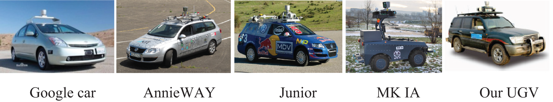
Recently, 3-D LiDARs have become more and more important for detecting obstacles by ALVs. In current mainstream ALV teams, including Stanford’s Junior,²⁸ KIT’s AnnieWAY,²⁶ Google self-driving car, the vehicle used in the study of Häselich et al.,²⁹ and our team³ (shown in Figure 2), the velodyne HDL-64E LiDAR is widely employed for obstacle detection. In these applications, their 3-D LiDARs are all uprightly fixed on their ALV platforms.

Figure 2.

3-D LiDARs are all uprightly fixed on current mainstream ALVs. ALVs: autonomous land vehicles.

The shortcoming of uprightly fixed LiDAR

In the aforementioned applications, 3-D LiDAR is always fixed uprightly on its ALV platform. There is a serious shortcoming: In this uprightly setup, LiDAR cannot view the region around the vehicle, which is sheltered from the body of vehicle itself. The vehicle would not be suffered from the blind area when it drove in flat environments or structured environments, since roads in these scenarios are structured and flat. The borders of the road on two sides could also help to keep the vehicle safe.³⁰ However, in a field environment, roads are usually narrow and unstructured with stakes and pits. Thus, the blind area would cause serious damages to the vehicle.

Under the traditional upright setup, the blind region around the vehicle can be analyzed as follows (Figure 3): The distance from the blind region to the side of the vehicle is B ₁ = W ₁ × (H ₁ + H ₂)/H ₁ − W ₁, where W ₁ is the half-width of the vehicle, H ₁ is the height of the mounted LiDAR, and H ₂ is the height of the vehicle. The size of the blind region in front of the vehicle is B ₂ = W ₂ × (H ₁ + H ₂)/H ₁ − W ₂, where W ₂ is the distance from the LiDAR to the head of the vehicle. The blind region is shown in Figure 3.

Figure 3.

Analysis on the blind area between two setups of 3-D LiDAR: (a) side view and (b) front view.

The details of the proposed new setup

Considering the shortcoming brought by traditional upright setup, in order to make a full use of LiDAR sensor, this article presents a new setup, that is, to make the LiDAR tilt on the side of the vehicle. The introduced new setup is described in Figure 1: Two compacted 3-D LiDARs are fixed on each side of the vehicle top—one is toward the left and another is toward the right. Both are equally angled forward.

There are three rules to obey for this new setup: (1) Make sure that no lasers from two LiDARs illuminate each other directly; otherwise, the sensors will be damaged; (2) the visual range around the vehicle depends on θ (Figure 4(a)); and (3) the visual range in front of the vehicle and the region of overlapped scans depends on φ (Figure 4(b)). The visual range with the proposed setup is shown in Figure 4, in which angles and their corresponding visual ranges are shown on two viewpoints: a front view and a top view. The overlapped area, labeled in Figure 4(b), greatly improves the capability of detection.

Figure 4.

The details of the proposed new installation method of LiDar. The scan region of LiDAR depends on θ and φ: (a) front view and (b) top view.

From Figure 4(b), we can see that the blind area around the vehicle is markedly reduced. The region on two sides of the vehicle is now visible to the relevant LiDAR. The front region is scanned and overlapped by both LiDARs, which greatly enhances the resolution and improves the capability of scene understanding. Under this setup, the geometrical characters of the obstacle in the LiDAR data become much more distinct than that under the traditional way. With this new setup, obstacle detection becomes more reliable and easy.

Comparative experiments between two setup methods

Several experiments are carried out to compare two different setup methods. As shown in Figure 1, two HDL-32E compact LiDARs are fixed as the new setup and an HDL-64 LiDAR is fixed as mainstream traditional upright setup. The HDL-64 LiDAR is chosen for comparison. Fifteen plastic pillars are placed around the platform as simulated objects, whose height is 0.5 m. As shown in Figure 5, those plastic pillars are used to test the view range and scan density for all of these LiDARs.

Figure 5.

The description of the designed comparing experiment: two different setup methods of LiDARs and the distribution of simulated obstacles.

Figure 6(a) describes the detect result by two HDL-32 LiDARs, in which we can know that 87% (13 obstacles) of obstacles are detected, and none of those most important obstacle is lost. Here, the most important obstacles for a vehicle are defined as follows: these obstacles that are near the vehicle would be firstly come into collision with the vehicle. Meanwhile, several obstacles may be ignored by the LiDAR, as in the traditional upright setup. Among those missed obstacles, the obstacles placed in two sides of the vehicle are important obstacles, which would cause serious damage to the vehicle when it takes a turn. From the comparative experiment, we can see that the new setup is really useful and brings a beneficial development to the ALV.

Figure 6.

The results of the designed comparison experiment: (a) shows the result of obstacle detection by the new setup, and (b) shows the result of obstacle detection by the upright setup.

Another experiment is carried out to show the view range under two different setup methods. Figure 7 shows the view range of both kinds of setup methods: The red and blue lines in Figure 7 are generated by the LiDARs under proposed setup method, while the green lines are generated by the LiDAR under upright setup method. From Figure 7, we can see that the LiDAR view range under the proposed setup method is much useful for a field ALV. When a vehicle is driven in a field environment, its speed must be limited, and the road is commonly narrow. Thus, these obstacles around the vehicle have the highest priority level to be detected to keep the vehicle safety. The proposed setup method is suitable for this requirement of field ALVs.

Figure 7.

The comparison of the view range generated by two different setup methods: the red and blue lines are generated by the LiDARs that under proposed setup method, the green lines are generated by the LiDAR that under upright setup method.

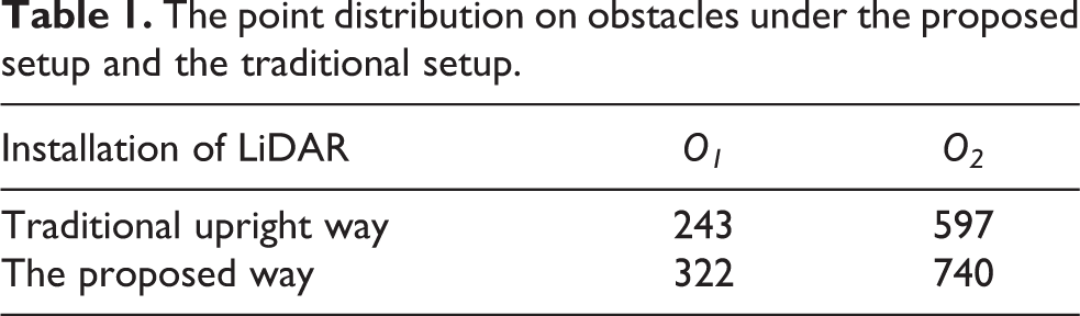
Another advantage of the proposed setup is that the scan line is much denser in the range of interest. With this new setup, the scan range in front of the vehicle overlaps in the experiment, which means more scan points are distributed in this region. Thus, the proposed setup improves the resolution of the LiDAR for obstacle detection. An experiment is specially designed to demonstrate this improvement (Figure 8): Two obstacles (one of them is a person) are standing in front of the vehicle: one is 6 m away from the vehicle, labeled as O ₁ and the other is 9 m away, labeled as O ₂. Both obstacles can be viewed by three LiDARs.

Figure 8.

The comparison of experiments for obstacle detection of two setups. (a) shows the result generated by the proposed setup, and (b) shows the result generated by the traditional setup.

In order to demonstrate the benefit of this proposed setup, the number of LiDAR points located on obstacles is listed in Table 1. From Table 1, we can read that obstacles get more distributed LiDAR points under the proposed setup, which means the two obstacles are more easily detected under the proposed setup.

Table 1.

The point distribution on obstacles under the proposed setup and the traditional setup.

Installation of LiDAR	O₁	O₂
Traditional upright way	243	597
The proposed way	322	740

A mathematical model to simulate the point distribution under the new setup

As mentioned earlier, the density of scan line is greatly developed when LiDARs are fixed under this new setup. Based on this setup, a mathematical model is deduced in order to simulate the distribution of scan points from a single line.

Analysis of difference of point distributions between two setups

By analyzing the working theory of LiDAR, the process of a LiDAR to detect a typical obstacle can be shown as in Figure 9(a), in which L represents the obstacle’s height and H represents the height that the LiDAR is placed on the vehicle. Several scan lines generated by the LiDAR are also described in Figure 9(a), which are distributed over the target obstacle. Here, D describes the distance from the obstacle to the vehicle.

Figure 9.

Analysis the difference of point distributions between two different installation methods: (a) shows the distribution of scan points when detecting an obstacle; (b) shows the distribution of scan points when LiDAR is upright fixed; and (c) shows the distribution of scan points when LiDAR is installed with new method.

In our algorithm, three cues are employed to detect obstacles. Firstly, the difference from adjacent scan points is a useful cue to reflect the changes in this scan line. For example, when there is an obstacle, the distance between adjacent points would change into shorter than normal. This phenomenon can be seen in Figure 9(a): $d_{P_{2} P_{3}}$ is much shorter because there is an obstacle (the normal distance should be $d_{P_{2}^{'} P_{3}^{'}}$ ). Another cue is that the distance of scan points ( $d_{P_{4} P_{5}}$ ) that followed the obstacle also would be unusual, which would be larger than normal. From Figure 9(a), we can see that $d_{P_{4} P_{5}}$ is seriously larger than $d_{{p^{'}}_{4} P_{5}}$ . The third cue applied in our algorithm is the height of an obstacle. It is obvious that these scan points would be higher than normal when they are located on an obstacle (P ₂, P ₃, P ₄ are higher than P ₁, P ₅, for instance). This cue would be easily impacted in filed environment. Thus, in our algorithm, these cues are combined as a whole character for judging whether it is an obstacle.

Scan lines are distributed on different ways by different setup methods. Figure 9(b) shows the scan points under upright setup, and Figure 9(c) shows the scan points under new setup. From Figure 9(b), we can see that these scan points (P₁, P₂, P₃, P₄), which are located on the potential obstacle, are from different lines. Meanwhile, Figure 9(c) shows that these scan points (P ₁, P ₂, P ₃, P ₄), which are located on the potential obstacle, are generated by the same line. From the intrinsic parameter of LiDAR, we can know that those adjacent points must be much denser when the LiDAR is fixed under proposed setup than that of traditional setup.³¹ Therefore, it can detect smaller obstacles under the new setup.

Deduced mathematical model to simulate a single scan line

When LiDAR is fixed under the new setup, its coordinate should be calibrated into the vehicle coordinate first.³² Then, the position of each scan point in vehicle coordinate can be computed. So, the distribution of scan points can be analyzed:

(1) From the attribute of the LiDAR, it is obvious that the angle between adjacent points is a constant value. Thus, θ_i (Figure 10) can be computed as follows (equation (1)).

Figure 10.

θ_i between two adjacent echo points from the same scan line.

In Figure 10, under the proposed setup, LiDAR scan line is scanning around a circle, and $θ_{i}^{'}$ depends on the number M, which is a LiDAR’s intrinsic parameter. Thus, $θ_{i}^{'} = 360 ° / M$ , where β_i is another LiDAR’s intrinsic parameter

sin (θ_{i} / 2) = sin (θ_{i}^{'} / 2) * cos (β_{i})

(2) There are many scan points between the obstacle and the vehicle for a scan line. If t is used to label the point number, then it means the t-th point is located on the obstacle, and D is used to express the distance from the obstacle to the vehicle, so the relationship of D and t can be expressed as equation (2). In the following equation, H represents the height of the fixed LiDAR

t = atan (D / H) / θ_{i}

(3) Another important information is the distance between each adjacent points, which can be described as W = P(t + 1) − P(t). Here, P(t) = D and P(t + 1) can be easily computed according to the following equation

P (t + 1) = tan (atan (D / H) + θ_{i}) * H

(4) The number of scan points located on the obstacle Num can be expressed as follows

{\begin{array}{l} t_{1} = atan (D / H) / θ_{i} \\ t_{2} = atan (D / (H - L)) / θ_{i} \\ Num = t_{2} - t_{1} \end{array}

(5) Synthesizing these aforementioned analyses, it can be deduced that the mathematical model of the point distribution for a scan line is denoted in equation (5). In the following equation, x represents the distance from the obstacle and the vehicle and y represents the height of scan point

{\begin{array}{l} t = atan (D / H) / θ_{i} \\ Num = atan (D / (H - L)) / θ_{i} - atan (D / H) / θ_{i} \\ x (t) = D \\ x (t + 1 : t + Num) = D \\ y (t) = 0 \\ y (t + i) \approx L * i / Num; i \in [1, Num] \end{array}

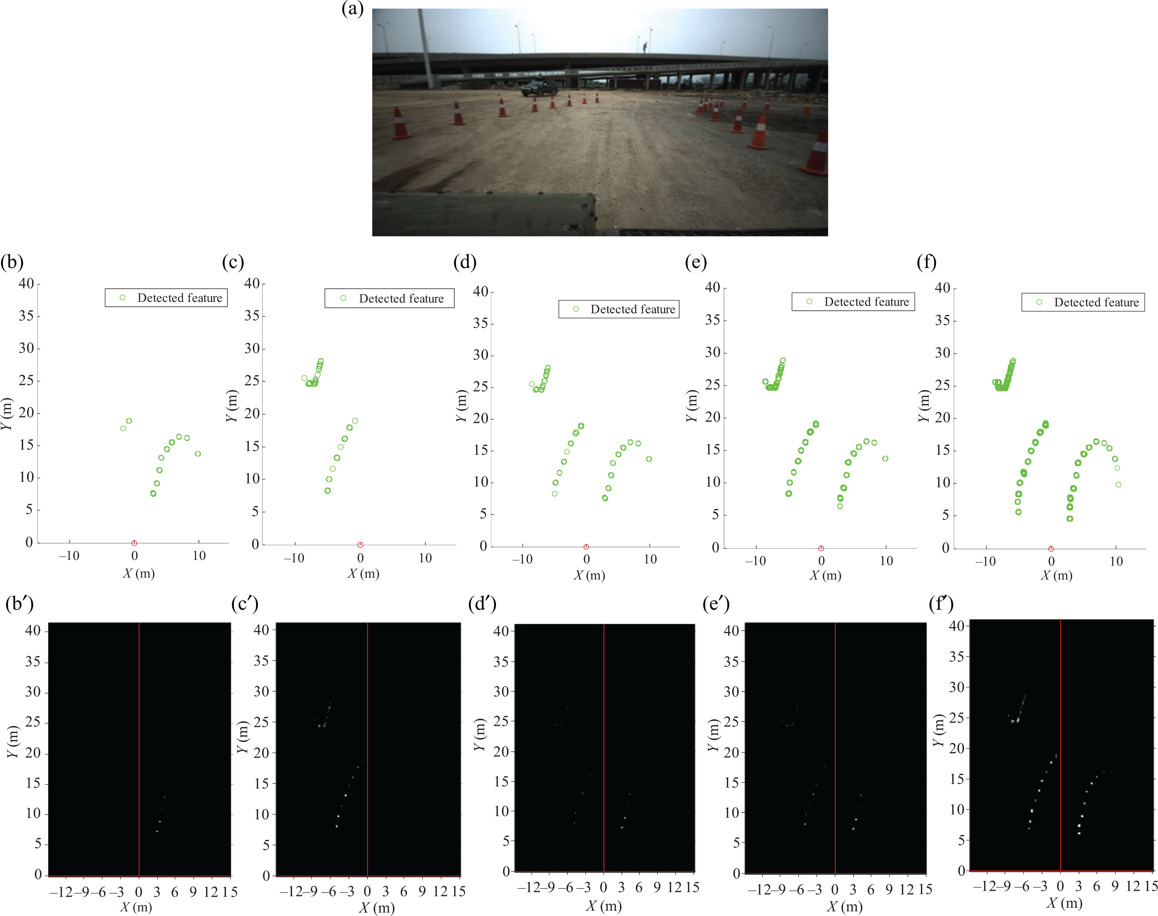
Therefore, simulated scan line can be generated according to the deduced mathematical model. In order to verify the performance of the deduced mathematical model, both simulated scan line and real scan line and their features are listed in Figure 11. A scenario with several obstacles around the vehicle is employed to implement this experiment (as shown in Figure 11(a)). The simulated scan line is listed in Figure 11(b), and the corresponding features are listed in Figure 11(c). The real scan line from the LiDAR and their corresponding features are also listed in Figure 11(d) and (e) for comparison. From these figures, we can see that the simulated scan line and their features are very similar to the real one. Thus, the deduced mathematical model is effective.

Figure 11.

The comparison of scan point distribution between real scan line and the simulated one: (a) experimental scene (a target is placed in front of the vehicle), (b) the ith line wave from the deduced mathematical model, (c) features of the ith line from the deduced mathematical model, (d) the ith line from real data, and (e) features of the ith line from real data.

The FMF-based algorithm for obstacle detection

The proposed FMF algorithm can be mainly divided into two parts: feature matching and feature fusion. The idea of feature matching can be described as follows: Each scan line can be regarded as a wave of signal. Thus, the problem of obstacle detection can be transformed into a problem of signal detection to detect these pulses in a signal wave. In the field of signal detection, a usual tool is matching filter to detect these pulses in a signal wave. So, the proposed algorithm employs these features that are generated by the simulated scan line to match the real one, and where there is a potential obstacle, there would be a peak. The idea of feature fusion can be described as follows: To make the detected obstacle more robust, the detect results are accumulated from different scan lines, different LiDARs, and different frames and are fused into a global map under a framework. Each feature would be assigned a different confidence according to Bayesian rule during its accumulating process. Then, potential obstacles are detected from this accumulated map finally.

Part 1: Feature matching to detect the potential obstacle

The first part of the FMF algorithm is to primarily detect the potential obstacle by matching features between real scan line and the simulated scan line. The mathematical model of FMF can be expressed as F(H, D, L, i), here D represents the distance from the vehicle to the obstacle, H represents the height of the mounted LiDAR, L denotes the height of the obstacle, and i represents the mathematical model corresponding to ith line. Thus, the step of this algorithm can be briefly summarized as follows:

Input: (1) a real scan line data from LiDAR; (2) F(H, D, L, i), the deduced model;

Step 1: Using the deduced model to generate a set of simulated scan lines for ideal obstacle, labeled as F_DL :

(1) change the distance D from RangeD1 to RangeD2, where RangeD1 and RangeD2 represent the minimal distance and themaximal distance of the obstacle that can be detect in this algorithm; and

(2) change the height L from RangeL1 to RangeL2, where RangeL1 and RangeL2 represent the minimal height and the maximal height of the obstacle that can be detect in this algorithm.

Step 2: Change both simulated scan line and real scan line into their corresponding features:

(1) change the real data W_i into its corresponding feature wave P_i ; and

(2) change all simulated scan lines F_DL into their corresponding feature wave P_DL .

Step 3: Matching all P_DL with each P_i , and a 2-D space is applied to accumulate the results, where the size of this parameter space is depended on the value D-L and their step size;

Step 4: When the results are accumulated in this parameter space, peak would emerge if there exists a potential obstacle. Thus, by detecting the peak, the potential obstacle would be detected, and the position of the peak denoted the size and the position of the detected obstacle;

Return: The size and the position of the detected obstacle (D_R , L_R ), if there is.

The key point of this algorithm is the simulated scan line and their features. Some classical feature waves P_DL , which are generated from a series of simulated can lines, are listed in Figure 12.

Figure 12.

Several classical characteristic curves P_DL of a potential obstacle: (a) L = 0.3, D = [2:1:15]; (b) L = 0.5, D = [2:1:15]; and (c) L = 0.7, D = [2:1:15].

Here, the two most common features, the height feature L and the width feature D, are employed, for example. Both L and D are traversed with a fixed step in a fixed range. The X axis in Figure 12 represents the series of scan points, which can be considered as the step of time for a wave. The t represents the step of time in X axis. The Y axis in Figure 12 represents the distance between adjacent scan points. All of those waves P_DL are used to match with the real feature wave that is generated from the real scan line. Therefore, if there is a potential obstacle, a peak would emerge in the 2-D parameter space.

In our experiments, the parameter D is set as D ∈ [2 m, 40 m] and the step size of D is set to be 0.5 m beforehand; the parameter L is set in [0.2 m, 1 m] and the step size of L is set as 0.2 m beforehand. It means that only those obstacles, which are placed in the range of 2–40 m away from the vehicle and their height is in the range of 0.2–1 m, can be detected by the proposed algorithm. There are two reasons: firstly, the range and size of target to be detected has included almost all the obstacles dangerous enough for vehicles. Secondly, the algorithm is required to work in real time. Thus, the 2-D parameter space [D_R, L_R ] cannot be too large in real application.

Some outdoor experiments are also employed to test this part of the proposed FMF algorithm. Our ALV is shown in Figure 1, and a pair of LiDARs are equipped at two side of the vehicle with the height H = 2 m. Some pillars are placed as obstacles in front of the vehicle (shown in Figure 13(a)). The detect results of two LiDARs are listed in Figure 13(b) and (c). The obstacles detected by the proposed algorithm in this scene are labeled by blue circles on the original LiDAR data. From the experimental results, we can see that the proposed algorithm for obstacle detection at different distances is stable and effective.

Figure 13.

The experimental results show the effectiveness of the proposed algorithm in real outdoor environment: (a) scene, (b) the detect results by left LiDAR, and (c) the detect results by right LiDAR.

Part 2: Feature fusion to improve the ability of the proposed algorithm

As mentioned earlier, the feature fusion-based algorithm is mainly applied to improve the ability of detection, which is based on the feature matching-based algorithm. The feature of potential obstacle detected in part of feature matching-based algorithm is used as the input for this part of the algorithm. Its framework can be described in Figure 14.

Figure 14.

The skeleton of the proposed algorithm.

Figure 14 shows the whole framework of the proposed FMF algorithm. The FMF algorithm fuses all features that are detected from different scan lines, different LiDARs, or even different frames into a global map according to the global positioning system (GPS) information. Before its accumulation, each detected feature would be estimated firstly, according to the relationship between adjacent features and history features by Bayesian rule. Meanwhile, for detecting obstacle more directly perceived through the senses, this global map is always changed into the current map, which obeys the vehicle coordinate. Then, peaks are found in this 2-D map, which is the position of the detected obstacles.

A real experiment is carried out in field environment to describe the process in real application of the proposed FMF algorithm, as shown in Figure 15. The test scenario included several typical obstacles, such as some pillars, another vehicle, a dam, and forest on the right side of the road, as shown in Figure 15(a). The original scan line data from the left LiDAR are listed in red color in Figure 15(b), and the detected obstacles are labeled by circles in green color. From the results, we can see that part 1 of the proposed FMF algorithm is effective, and nearly all obstacles are detected. The same of right LiDAR is listed in Figure 15(c). Two maps, the global map and the current map, are listed in Figure 15(d) and (e). The main reason for fusing all features into the global map is that these features may come from different LiDARs at different times, and they need to be under a same coordinate. The exchange operation between the current map and the global map depends on GPS information; for each scan, frame has its own GPS information when data are captured. The parameter space that accumulated all of these features with their weights is shown in Figure 15(f), and the potential obstacle is detected from Figure 15(f) by finding the peaks, which is shown in Figure 15(g).

Figure 15.

The process of this algorithm. (a) shows a scenario that has several positive obstacles. (b) shows the original data and its detection results by left LiDAR. (c) shows the original data and its detection results by right LiDAR. (d) shows the global map. (e) shows the current map. (f) shows the parameter space. Peaks are analyzed in (f), and the result of obstacle detection is shown in (g).

There are two novel points of this part of the proposed FMF algorithm: firstly, fusing all features, which are from different scan lines at different times, into a global map. On the one hand, this novelty greatly improves the robustness and stability of the proposed algorithm. On the other hand, it does not require two LiDARs to be synchronous any more for this algorithm. Secondly, weight generation is another novel point, which is generated according to the Bayesian rule. Thus, different features are assigned different values of weight.

Bayesian rule is very classic

P (A | X_{i}) = \frac{P (X_{i} | A) P (A)}{P (X_{i})}

When multi-cues is applied, equation (6) should be rewritten as

P (A | X_{i}, X_{i + 1}) = \frac{P (X_{i + 1} | A, X_{i}) P (X_{i} | A) P (A)}{P (X_{i + 1} | X_{i}) P (X_{i})} = \frac{P (X_{i + 1} | A, X_{i})}{P (X_{i + 1} | X_{i})} P (A | X_{i})

From the rule of probability, equation (7) can be rewritten as follows

P (A | X_{i}, X_{i + 1}) = \frac{P (X_{i + 1} | A, X_{i})}{P (X_{i + 1} | A, X_{i}) P (A | X_{i}) + P (X_{i + 1} | \sim A, X_{i}) P (\sim A | X_{i})} P (A | X_{i})

The process of obstacle detection might be thought that a set of scan lines are employed to independently find potential obstacle. Thus, $P (X_{i + 1} | A, X_{i}) = P (X_{i + 1} | A)$ . Thereby, equation (8) can be translated as follows

P (A | X_{i}, X_{i + 1}) = \frac{P (X_{i + 1} | A)}{P (X_{i + 1} | A) P (A | X_{i}) + P (X_{i + 1} | \sim A) P (\sim A | X_{i})} P (A | X_{i})

In equation (9), X represents the ith feature; A represents the feature that be an obstacle; $P (A | X_{i})$ represents the probability to be an obstacle, which is from the exited global map; and $P (X_{i}_{+ 1} | A)$ represents the probability to be an obstacle, which depended on the current detection. $P (X_{i + 1} | \sim A)$ is a probability of likelihood to describe that it is not an obstacle, which is depended on the deduced mathematical model.

An example is employed to show how to use the Bayesian rule in the proposed FMF algorithm. Suppose $P (X_{i + 1} | \sim A) = 0.7$ to describe the probability to be an obstacle for each detected feature, and suppose the prior probability $P (X_{i + 1} | \sim A) = 0.1$ , and the global map is set $P (A) = P (A | X_{0}) = 0.01$ beforehand. According to equation (9), iterating process can be described as follows

{\begin{array}{l} P (A | X_{1}) = \frac{P (X_{1} | A)}{P (X_{1} | A) P (A | X_{0}) + P (X_{1} | \sim A) P (\sim A | X_{0})} P (A | X_{0}) = \frac{0.7}{0.7 \times 0.01 + 0.1 \times (1 - 0.01)} \times 0.01 = 0.066 \\ P (A | X_{2}) = \frac{P (X_{2} | A)}{P (X_{2} | A) P (A | X_{1}) + P (X_{2} | \sim A) P (\sim A | X_{1})} P (A | X_{1}) = \frac{0.7}{0.7 \times 0.066 + 0.1 \times (1 - 0.066)} \times 0.066 = 0.3311 \\ P (A | X_{3}) = \frac{P (X_{3} | A)}{P (X_{3} | A) P (A | X_{2}) + P (X_{3} | \sim A) P (\sim A | X_{2})} P (A | X_{2}) = \frac{0.7}{0.7 \times 0.3311 + 0.1 \times (1 - 0.3311)} \times 0.3311 = 0.776 \\ P (A | X_{4}) = \frac{P (X_{4} | A)}{P (X_{4} | A) P (A | X_{3}) + P (X_{4} | \sim A) P (\sim A | X_{3})} P (A | X_{3}) = \frac{0.7}{0.7 \times 0.776 + 0.1 \times (1 - 0.776)} \times 0.776 = 0.96 \\ P (A | X_{5}) = \frac{P (X_{5} | A)}{P (X_{5} | A) P (A | X_{4}) + P (X_{5} | \sim A) P (\sim A | X_{4})} P (A | X_{4}) = \frac{0.7}{0.7 \times 0.96 + 0.1 \times (1 - 0.96)} \times 0.96 = 0.994 \end{array}

From equation (10), we can see that the obstacle can be affirmed by five lines scanned on it, the proposed algorithm would consider it is 99.4% to be an obstacle.

Figure 16 describes the process of applying Bayesian rule by using a real test. Figure 16(a) illustrates the scenario for experiments, in which a set of obstacles are placed. The detect results from part 1 of the FMF algorithm are listed in Figure 16(b) to (f). According to the proposed algorithm, these results would be assigned different weights according to the Bayesian rule and be accumulated in the global map, which are shown in Figure 16(b′) to (f′). Five cases are listed to illustrate the process: Figure 16(b) and (b)′ is in case of a frame from left LiDAR, Figure 16(c) and (c′) is in case of a frame from right LiDAR, Figure 16(d) and (d′) is in case of fusing each frame together from both LiDARs, Figure 16(e) and (e′) is in case of fusing two adjacent frames together from two LiDARs, and Figure 16(f) and (f′) is in case of fusing five adjacent frames together from two LiDARs. It is obvious that when accumulating five frames, the probability of these obstacles is achieved almost 100% (shown in Figure 16(f′)).

Figure 16.

The details of applying Bayesian rule to detect obstacles in the global map. (a) illustrates the scenario that a set of obstacles are placed. The detect results from part 1 of the FMF algorithm are listed in (b) to (f). The global map which describes the process of applying Bayesian rule is shown in (b′) to (f′).

Performance evaluation

In order to verify the performance of our algorithm, a set of experiments are designed. There are three components: In part I, the software of interface applied in our experiment is firstly introduced, and the definition of detection accuracy and distance is discussed. Then, kinds of scenarios both including structured environment and field environment are employed to evaluate the performance of the introduced FMF algorithm and compared with some state-of-the-art algorithms in part II. In part III, detecting the dynamic obstacles is specially discussed.

Part I: Introduction of software’s interface and definition of detection accuracy and distance

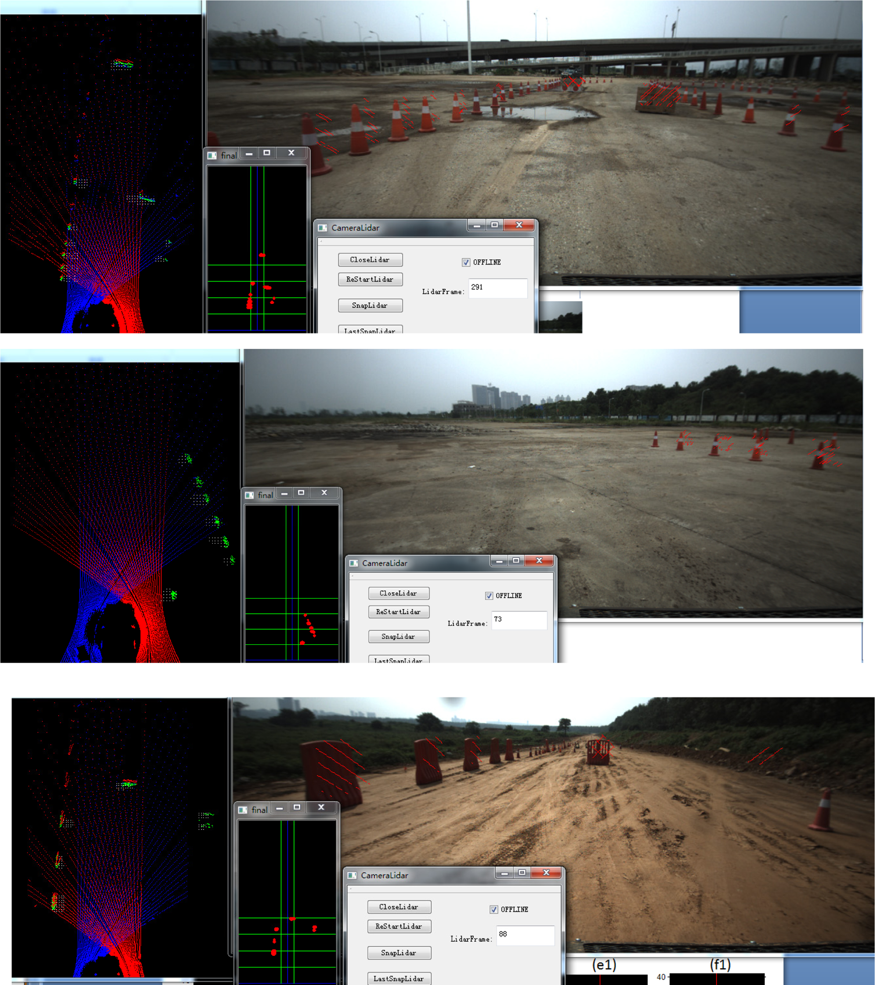
In order to carry out the designed experiment, a friendly interface is very important to show information. The interface of our software is composed of four parts and several tools of labels (Figure 17). They are the LiDAR’s view (Figure 17(a)), the grid map view (Figure 17(b)), the control platform (Figure 17(c)), and the color camera view (Figure 17(d)). In the LiDAR’s view, original scan lines are given in blue (from the left LiDAR) and in red (from the right LiDAR). The result of obstacle detection by the proposed algorithm is also labeled on those original data by using green lines. The grid map view is also employed to show the result of obstacle detection, which is under the vehicle coordinate. The coordinate resolution is defined as follows: The cross of the two blue lines is the origin of coordinate, and each grid denotes 0.2 m × 0.2 m. Several colored lines are applied to mark the distance more clearly, in which the row green line represents 5 m and column green line represents 2 m distance. The detected obstacles are labeled as red grid in this map. The control platform is mainly used to control the experiment, such as start the LiDAR work or stop the LiDAR, and shows the frame number and so on. The color camera view is employed to show the scene more clearly for human. Thus, the color camera is not joined for obstacle detection. In order to show the results of detection more vividly, the detected obstacle would also be labeled in this view by red line in image, according to the mapping ship between the camera and the LiDAR. In addition, the camera is not required to be strictly synchronous with LiDARs. That is the reason that the result of the proposed algorithm labeled in the color image does not match the obstacle strictly.

Figure 17.

The interface of the software tool. (a) shows the LiDAR’s view, (b) shows the grid map view, (c) shows the control platform, and (d) shows the color camera view.

Figure 18 illustrates the process of detecting an obstacle: When a vehicle is driven toward the obstacle, more and more points would locate on the obstacle when the vehicle is approaching the target. The variety of the point number recorded in the grid map is shown in Figure 18. Thus, the detected obstacle is known in every time when the detect process changes from far to near. Figure 18 shows this process of the vehicle from far to near. X axis denotes the distance from the obstacle to the vehicle, and Y axis describes the point number located on the obstacle.

Figure 18.

The process of detecting an obstacle when the vehicle approaches the target.

For a target, when a fixed number of points (a threshold set beforehand) are detected on a region, it would be considered as a potential obstacle. As shown in Figure 18, this obstacle in the experiment is detected at a distance of 35 m away from the vehicle. This distance is defined as the maximal detect distance by the proposed algorithm.

Part II: Adaptability analysis

In this part, various obstacles in different scenes are employed to evaluate the adaptability and the ability of the presented FMF algorithm. Two different ALVs are employed, LiDARs are mounted on different heights, one is on H = 1.4 m and another is on H = 2 m. HDL-32 LiDAR is employed as the sensor in our experiment, and a pair of them is mounted according to the proposed new setup.

A lot of experiments are carried out in both cement roads and field roads. Several typical results are as shown in Figures 19 and 20. The detected results are marked in all of three view windows: in the LiDAR’s view, the grid map view, and the color image view. In our experiment, many obstacles existed in the tested scene, so they are not the maximal detection distance for the proposed algorithm. From these experimental results, it is obvious that the presented FMF algorithm has a satisfactory performance.

Figure 19.

Experimental scene and the detection results (I).

Figure 20.

Experimental scene and the detection results (II).

Consider the maximal detection distance of a positive obstacle is meaningless, because it depends on the size of the obstacle and the kind of sensors. For example, if the obstacle is big and high enough, and it is intervisible between the sensor and the obstacle, then the maximal detection distance is mainly determined by the ability of the sensor, rather than the ability of algorithms. Therefore, this article mainly compares the computing time with other approaches, but not the maximal detection distance.

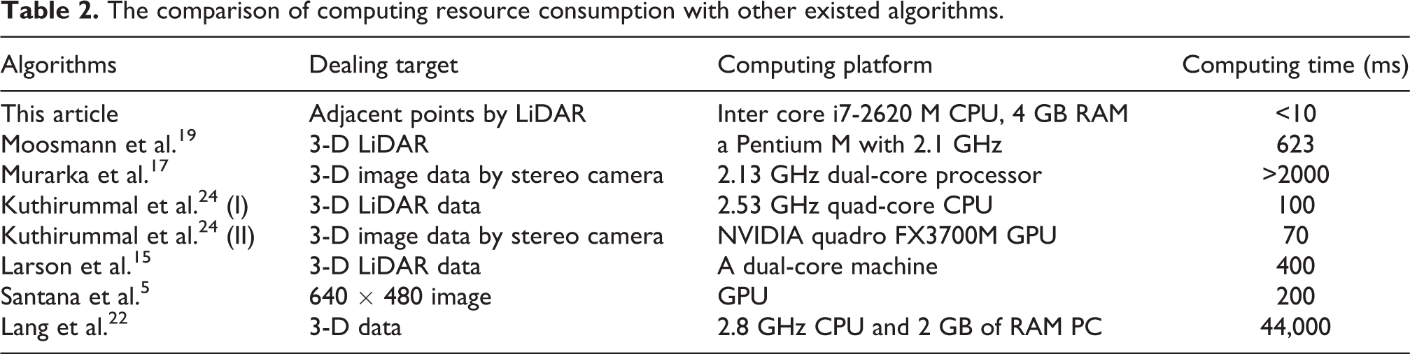
Computing time of a detection algorithm is very important for ALVs. The main computing operation of the proposed FMF algorithm is based on adjacent points; thus, its required computing resource is very low. With an Intel dual-core i7-2620M CPU and 4 GB RAM computer, it costs less than 10 ms. Some comparison is carried out as follows: 3-D LiDAR is also employed in the study of Moosmann et al.,¹⁹ in which the algorithm is worked on a Pentium M with 2.1 GHz processor, and it costs about 623 ms. Murarka et al.¹⁷ used a 3-D image data generated from a stereo camera to implement the same task, and it costs more than 2000 ms on a 2.13 GHz dual-core processor. Kuthirummal et al.²⁴ tested their algorithm using 3-D LiDAR data and 3-D image data from a stereo camera. The algorithm dealing with 3-D LiDAR data is worked on a 2.53 GHz quad-core CPU, and its computing time is about 100 ms. While the same algorithm deals with 3-D image data generated from a stereo cameras, it costs about 70 ms on a NVIDIA quadro FX3700 M GPU platform. Larson et al.¹⁵ also proposed an obstacle detection algorithm, in which LiDAR data were used, and its frequency was about 2.5 Hz on a dual-core machine platform. Another algorithm is introduced in the article.⁵ For a 640 × 480 image working on a GPU, it costs about 200 ms to finish a frame. The aforementioned computing time is listed in Table 2. By analyzing, our algorithm is one of the fastest algorithms among the known algorithms.

Table 2.

The comparison of computing resource consumption with other existed algorithms.

Algorithms	Dealing target	Computing platform	Computing time (ms)
This article	Adjacent points by LiDAR	Inter core i7-2620 M CPU, 4 GB RAM	<10
Moosmann et al.¹⁹	3-D LiDAR	a Pentium M with 2.1 GHz	623
Murarka et al.¹⁷	3-D image data by stereo camera	2.13 GHz dual-core processor	>2000
Kuthirummal et al.²⁴ (I)	3-D LiDAR data	2.53 GHz quad-core CPU	100
Kuthirummal et al.²⁴ (II)	3-D image data by stereo camera	NVIDIA quadro FX3700M GPU	70
Larson et al.¹⁵	3-D LiDAR data	A dual-core machine	400
Santana et al.⁵	640 × 480 image	GPU	200
Lang et al.²²	3-D data	2.8 GHz CPU and 2 GB of RAM PC	44,000

Part III: Analysis of detecting dynamic obstacles

Environment is an open aggregation, and there are two kinds of obstacles: static obstacles and dynamic obstacles. The proposed algorithm mainly focuses on these static obstacles. In field environment, dynamic obstacles, such as people or other vehicles, are not very common. That is to say, the algorithm proposed in this article is mainly for our ALV to join the round unmanned vehicle challenge of China, and the ALV is tested mainly on field environment and very few dynamic obstacles are emerged in this challenge.

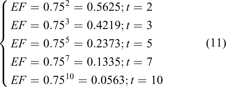
According to the theory of the proposed algorithm, the detect result in each frame would translate into a global map according to GPS information. Thus, this method is not suitable for detection dynamic obstacles in theory. In order to deal with this problem (also for avoiding error result in single frame), the decline factor is applied to decline the effect of history results. The decline factor is set 0.75 for obstacle detection here. The effect factor for history detection results is EF = 0.75 ^t , where t represents the frame generated t times ago. Several effect factors in different frames are shown in equation (11). In the following equation, we can see that there is almost no effect from the result generated t = 10 ago

{\begin{array}{l} E F = {0.75}^{2} = 0.5625; t = 2 \\ E F = {0.75}^{3} = 0.4219; t = 3 \\ E F = {0.75}^{5} = 0.2373; t = 5 \\ E F = {0.75}^{7} = 0.1335; t = 7 \\ E F = {0.75}^{10} = 0.0563; t = 10 \end{array}

In order to verify the analysis mentioned earlier, real experiments are designed as follows: a flat-bed trailer, as a typical dynamic obstacle, pulled and pushed in two sides in front of the ALV, testing the effectiveness of the proposed algorithm for detecting dynamic obstacles. Experimental results are as shown in Figures 21 and 22, where (a) shows the scene where a flat-bed trailer is moving in front of the ALV. (b) and (c) show the scan points generated by two LiDARs, where the detected potential obstacles are labeled by green circles. (d) shows the current map, in which the detect results are cumulated from different LiDARs and on different frames. During the cumulation, decline factor is employed to reduce the noise brought from history frames. (e) shows the final result. The results from both scenes show that the proposed FMF algorithm is effective for dynamic obstacles when the relative speed between the obstacle and the vehicle is in a limited range (the maximal speed is not strictly tested, but the proposed algorithm works well under 40 km/h).

Figure 21.

The results for detecting dynamic obstacle (I).

Figure 22.

The results for detecting dynamic obstacle (II).

Conclusion

This article presents an obstacle detection algorithm by using a pair of compact LiDARs. A new setup of compact LiDAR is specially designed for obstacle detection in field environment. A mathematical model is deduced to simulate the distribution of the scan line. An FMF-based algorithm is introduced, and the experimental results show that the proposed algorithm is robust, stable, and effective. This algorithm has been successfully applied to our ALV, which won the challenge of Chinese Overcome Danger 2014 ground unmanned vehicle.³³

The main contribution of this article is as follows: One is its new setup and another one is its idea of dealing data by using adjacent points. Firstly, it must consider using more cheaper sensors instead of HDL-64 LiDAR, as it is too expensive for ALVs. The new setup shows that two compact HDL-32 LiDARs can replace an HDL-64, and their ability is much better from visual range and data density. It is believed that many cheaper LiDARs would emerge in future, and this new setup would be widely used. Second, the idea of dealing with data by using adjacent points is very useful, which needs less computing resource and is almost real-time implementation. In addition, another advantage of this idea is that it nearly cannot be affected by the field road surface and the bumpiness. All in all, it is hoped that this work would be beneficial for enhancing the development of field ALVs.

Footnotes

Declaration of conflicting interests

The author(s) declared no potential conflicts of interest with respect to the research, authorship, and/or publication of this article.

Funding

The author(s) disclosed receipt of the following financial support for the research, authorship, and/or publication of this article: This work is part support by National Nature Science Foundation (No.91220301).

References

Zhou

McDaniel

. Self-supervised learning to visually detect terrain surfaces for autonomous robots operating in forested terrain. J Field Robot 2012; 29(2): 277–297.

Shang

. Robust unstructured road detection: the importance of contextual information. Int J Adv Robot Syst 2013; 10(3): 1–88.

Wang

Chen

Dai

. Gaussian-process-based real-time ground segmentation for autonomous land vehicles. J Intell Robot Syst 2014; 76(3): 563–582.

Manduchi

Castano

Talukder

. Obstacle detection and terrain classification for autonomous off-road navigation. Auton Robots 2005; 18(1): 81–102.

Santana

Guedes

Correia

. Stereo-based all-terrain obstacle detection using visual saliency. J Field Robot 2010; 28(2): 241–263.

Doerr

Mohsenimanesh

Laguë

. Application of the LIDAR technology for obstacle detection during the operation of agricultural vehicles. Can Biosyst Eng 2013; 55: 2–9.

Tingbo

. Research on stereo vision algorithms and their application in obstacle detection for ALV. PhD Thesis, National University of Defense Technology, China, 2012.

Huertas

Rankin

Matthies

. Nighttime negative obstacle detection for off-road autonomous navigation. In: Proceedings of the international conference on intelligent robots and systems (IRS), 2007, pp. 906–913.

Sun

Bebis

Miller

. On-road vehicle detection: a review. IEEE Trans Pattern Anal Mach Intell 2006; 28: 694–711.

10.

Dalal

. Finding people in images and videos. PhD Thesis, Institut National Polytechnique de Grenoble-INPG, France, 2006.

11.

Abramson

Freund

. Active learning for visual object detection. University of California San Diego, San Diego, CA, CS2006-0871 Tech. Rep., 2006.

12.

Hoiem

Efros

Hebert

. Putting objects in perspective. In: IEEE computer society conference on computer vision and pattern recognition, Vol. 2, 2006, pp. 2137–2144. IEEE.

13.

Larson

Trivedi

. LIDAR based off-road negative obstacle detection and analysis. In: 14th international IEEE conference on intelligent transportation systems (ITSC), 2011, pp. 192–197. IEEE.

14.

Han

Kim

Lee

. Enhanced road boundary and obstacle detection using a downward-looking LIDAR sensor. Veh Technol IEEE Trans 2012; 61(3): 971–985.

15.

Larson

Trivedi

Bruch

. Off-road terrain traversability analysis and hazard avoidance for UGVS. Technical report, DTIC Document, 2011.

16.

Morton

Olson

. Positive and negative obstacle detection using the HLD classifier. In: IEEE/RSJ international conference on intelligent robots and systems (IROS), 2011, pp. 1579–1584. IEEE.

17.

Murarka

Sridharan

Kuipers

. Detecting obstacles and drop-offs using stereo and motion cues for safe local motion. In: IEEE/RSJ international conference on intelligent robots and systems, IROS 2008, 2008, pp. 702–708. IEEE.

18.

Puntambekar

. Terrain modeling and obstacle detection for unmanned autonomous ground robots, Ph.D. dissertation, 18 10 2006.

19.

Moosmann

Pink

Stiller

. Segmentation of 3D LIDAR data in non-flat urban environments using a local convexity criterion. In: Intelligent vehicles symposium, 2009 IEEE, 2009, pp. 215–220. IEEE.

20.

Douillard

Underwood

Kuntz

. On the segmentation of 3D LIDAR point clouds. In: IEEE international conference on robotics and automation (ICRA), 2011, pp. 2798–2805. IEEE.

21.

Hadsell

Bagnell

Huber

. Non-stationary space-carving kernels for accurate rough terrain estimation. Int J Robot Res (IJRR) 2010; 29(8): 981–996 .

22.

Lang

Plagemann

Burgard

. Adaptive non-stationary kernel regression for terrain modeling. In: Robotics: science and systems conference (RSS), Atlanta, Georgia, USA, October 2007.

23.

Vasudevan

Ramos

Nettleton

. Non-stationary dependent Gaussian processes for data fusion in large-scale terrain modeling. In: International conference on robotics and automation (ICRA), 9–13 May 2011, pp. 1875–1882. China: Shanghai.

24.

Kuthirummal

Das

Samarasekera

. A graph traversal based algorithm for obstacle detection using LIDAR or stereo. In: IEEE/RSJ international conference on intelligent robots and systems (IROS), 2011, pp. 3874–3880. IEEE.

25.

Thrun

Montemerlo

Dahlkamp

. Stanley: the robot that won the DARPA grand challenge. J Field Robot 2006; 23(9): 661–692.

26.

Kammel

Ziegler

Pitzer

. Team Annieway’s autonomous system for the 2007 DARPA urban challenge. J Field Robot 2008; 25(9): 615–639.

27.

Montemerlo

Thrun

. Large-scale robotic 3-D mapping of urban structures. In: Experimental robotics ix, Singapore, 18–21 6 2006, pp. 141–150. Springer.

28.

Montemerlo

Becker

Bhat

. Junior: the Stanford entry in the urban challenge. J Field Robot 2008; 25(9): 569–597.

29.

Häselich

Arends

Wojke

. Probabilistic terrain classification in unstructured environments. Robot Autonomous System 2013; 61: 1051–1059.

30.

Bagnell

Urmson

Anhalt

. Autonomous driving in urban environments: boss and the urban challenge. J Field Robot 2008; 25(8): 425–466.

31.

Velodyne LiDAR Inc. HDL-32E user’s manual, www.velodynelidar.com, 10 2012.

32.

Shang

Shi

. An efficient calibration approach for arbitrary equipped 3-D LIDAR based on an orthogonal normal vector pair. Journal of Intelligent Robot System 2015; 79: 21–36.

33.

Guancha. The “Overcome Danger 2014” ground unmanned vehicle challenge of China, http://www.guancha.cn/military-affairs.shtml, 5 2014.

A feature matching and fusion-based positive obstacle detection algorithm for field autonomous land vehicles

Abstract

Keywords

Introduction

Related works

A new setup method of compact LiDAR

The shortcoming of uprightly fixed LiDAR

The details of the proposed new setup

Comparative experiments between two setup methods

A mathematical model to simulate the point distribution under the new setup

Analysis of difference of point distributions between two setups

Deduced mathematical model to simulate a single scan line

The FMF-based algorithm for obstacle detection

Part 1: Feature matching to detect the potential obstacle

Part 2: Feature fusion to improve the ability of the proposed algorithm

Performance evaluation

Part I: Introduction of software’s interface and definition of detection accuracy and distance

Part II: Adaptability analysis

Part III: Analysis of detecting dynamic obstacles

Conclusion

Footnotes

Declaration of conflicting interests

Funding

References