Sage Journals: Discover world-class research

Abstract

The movement state of obstacle including position, velocity, and yaw angle in the real traffic scenarios has a great impact on the path planning and decision-making of autonomous vehicle. Aiming at how to get the obstacle’s movement state in the real traffic scenarios, an approach is proposed to detect and track obstacle based on three-dimensional Light Detection And Ranging (LiDAR). Firstly, the point-cloud data produced by three-dimensional LiDAR after the road segmentation is rasterized, and the reuse of useful non-obstacle cells is carried out on the basis of the rasterized point-cloud data. The proposed eight-neighbor cells clustering algorithm is used to cluster the obstacle. Based on the clustering result, static obstacle detection of multi-frame fusion is worked out by combining real-time kinematic global positioning system data and inertial navigation system data of autonomous vehicle. And we further use the static obstacle detection result to detect moving obstacle located in the travelable area. After that, an improved dynamic tracking point model and Kalman filter are applied to track moving obstacle stably, and we finally get the moving obstacle’s stable movement state. A large amount of experiments on the autonomous vehicle developed by us show that the method has a high degree of reliability.

Keywords

Autonomous vehicle 3-D LiDAR detection and tracking real-time kinematic global positioning system Kalman filter

Introduction

In recent years, with the development of artificial intelligence and robot technology, autonomous vehicle as an important branch of artificial intelligence has become a hot research field. Autonomous vehicle mainly uses camera, LiDAR, global positioning system (GPS), and other sensors to achieve real-time perception of the surrounding environment.¹ Obstacle detection and tracking is an important content of autonomous vehicle environment perception. And it is also an important basis for path planning and decision-making of autonomous vehicle.

Currently, the researches on obstacle detection and tracking mainly focus on computer vision^2
–4 and LiDAR.^5
–7 Vision-based object detection using deep learning method has been developed a lot,^8,9 but the computer vision-based approach is very susceptible to light, causing poor detection and tracking results when light is weak. LiDAR is widely used in the detection and tracking of autonomous vehicle as its extraordinary ability to obtain the basic shape, distance measurement, and position of the obstacle.

Yang¹⁰ established a box model containing the target center position, velocity, and so on to describe the obstacle’s movement state and adopted multi-hypothesis tracking algorithm to solve the problem of tracking multi-moving targets. But they do not take into account the fact that the point clouds will affect the precision of the center position during the tracking process, making the tracking result unsatisfactory. Xin et al.¹¹ combined three-dimensional (3-D) LiDAR and four-line laser sensor to detect and track moving obstacles around autonomous vehicle. They solved the problem existed in Yang’s work¹⁰ to some extent, but failed to find a stable tracking point during the movement of the obstacle, causing the severe change in yaw angle. In Himmelsbach and Wuensch’s study,¹² the oriented bounding box is used to describe the target obstacle. The RANSAC algorithm is used to find the principal component distribution direction of the segmented point clouds, and then the yaw angle of the obstacle is obtained. The results obtained by this approach are more stable than the results obtained by the method of Xin et al.¹¹ But they don’t provide initializing tracks with top-down knowledge, which may represent nonrigid obstacles inaccurately.

Ralf et al.¹³ propose a generative Bayesian approach for detecting dynamic objects, and they use an approach based on the Kalman filter to track dynamic objects. But they only show the results based on a static sensor. Frank and Christoph¹⁴ use a segmentation method based on local convexity for hypothetical object detection. They combine Iterative Closest Point (ICP) and a Kalman filter to track and classify the tracks. Anna and Sebastian¹⁵ use a model-based approach to vehicle detection and tracking from 3-D laser data alone. Their model is used for precise motion estimation, and the proposed approach does not require data association of obstacles.

This article proposes a new approach to improve static/moving obstacle detection and tracking. Firstly, road point-cloud data are removed from the point-cloud data of one frame and the reuse of useful non-obstacle cells is carried out, then, the proposed clustering algorithm is used to cluster the obstacle cells quickly. When it comes to obstacle detection, we detect static obstacles by multi-frame before detecting moving obstacles. And finally, the proposed dynamic tracking point model and Kalman filter algorithm are applied to track the moving obstacles. The good performance in the real urban scenarios shows that the proposed approach has high reliability and can detect and track moving obstacle well.

The remaining part is organized as follows. The second section describes obstacle clustering algorithm. Static obstacle detection is presented in the third section, and the fourth section describes the moving obstacle detection and tracking process. The fifth section presents experimental results and analysis, and the last section brings some conclusions.

Obstacle clustering

Obstacle clustering is an important basis for obstacle detection and tracking. HDL-64E LiDAR can produce nearly 130,000 point-cloud data per frame, which is a large amount of points that can characterize the spatial distribution and surface properties of the obstacle in the same spatial reference system. In the face of such a large amount of data, the point-cloud data should be preprocessed firstly and then clustered.

Point-cloud data preprocessing

Firstly, we adopt the method of Zhiyuan et al.¹⁶ to complete the road segmentation. Figure 1 is the result of road segmentation. The left figure is the original point-cloud data of one frame, and the right figure is the road segmentation result. After the road segmentation, the remaining point-cloud data are rasterized into cells, and we give each cell specific attribute values to distinguish them from each other.

Figure 1.

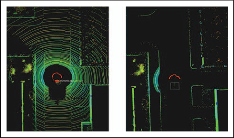
The left figure is the original point-cloud data, and the right figure is the road segmentation result.

The coordinate system which is used for point-cloud data rasterizing is shown in Figure 2, and we use the 40 cm × 40 cm cell to rasterize the remaining point-cloud data, creating a size of 200 × 200 grid occupancy map. After rasterizing the remaining point-cloud data, the attributes of each cell are assigned, including the number of points falling into the cell, the maximum point-cloud height, the minimum point-cloud height, and obstacle category of the cell. According to the quantity of points falling into the cell, the obstacle category of each cell is determined. Since the point-cloud data still have noisy points after the road segmentation, when the number of point clouds in a cell is 0, we are sure that the cell is indeed a non-obstacle cell. However, when there are few point clouds in a cell, the point-cloud data may represent the position of obstacle accurately, but may also contain noisy points which will lead to wrong detections. So, in order to avoid the effects from noisy points, we take two points as a threshold which is obtained through actual experiment to distinguish obstacle and non-obstacle cell. If the number of points in the cell is less than 2, the cell will be regarded as a non-obstacle cell and its category value is assigned to 0, or it will be regarded as an obstacle cell and its category value is assigned to 1. Through this step, the occupancy grid map will be created.

Figure 2.

Coordinate system for point-cloud data rasterizing.

Because of the spacing between different laser lines of HDL-64E, and over-segmentation of road, the point-cloud data of one frame after road segmentation cannot present the surrounding environment around autonomous vehicle precisely. Therefore, we add additional cells to enrich the useful information we once missed. If there are two obstacle cells whose intermediate cells are several non-obstacle cells, and one obstacle cell’s maximum point-cloud height is similar to the other, then we will change the intermediate non-obstacle cells into obstacle cells and assign the attribute values of the two obstacle cells to the non-obstacle cells. However, if the quantity of intermediate non-obstacle cells exceeds 3, no additional non-obstacle cell is changed into obstacle cell. When the LiDAR is installed at the position which is away about 2.2 m from the ground, the distance between different laser lines is about 2.3 m at the distance of 40 m away from autonomous vehicle, so changing possible non-obstacle cells into obstacle cells when the non-obstacle cells which are no more than three between two obstacle cells whose maximum point-cloud height is similar to the other is reasonable, as the maximum length of added obstacle cells is 1.2 m. Changing useful non-obstacle cells into obstacle cells can greatly enhance the ability of point-cloud data to present the surrounding environment around autonomous vehicle. Figure 3 is the occupancy grid map which has added additional useful cells. The middle blue box represents the position of autonomous vehicle, and the left figure is the original point-cloud data after road segmentation, and the right figure is the occupancy grid map with added cells.

Figure 3.

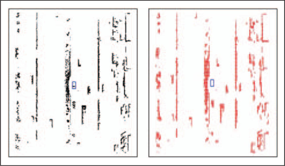
The left figure is the original point-cloud data after road segmentation, and the right figure is the occupancy grid map.

Eight-neighbor cells clustering algorithm

In this article, we propose an eight-neighbor cells clustering algorithm, which can quickly complete the cells clustering. As shown in Figure 4, the left lower cell with index (i, j) will be regarded as the first seed cell. After the cell (i, j) finished eight-neighbor cells search, the cell (i, j + 1) is added to the list table which is used to restore the encountered obstacle cells’ indexes, and the identification value of the seed cell (i, j) changes from 0 to 1, so when the cell (i, j + 1) is doing extended search, the cell (i, j) will not be added to the list table again since its identification value is 1. Meanwhile, the identification value of cell (i, j + 1) will become 1. Then, the next obstacle cell in the list table will be used as the new seed cell, and the loop will last until the final obstacle cell in the list table is used.

Figure 4.

The diagram of eight-neighbor cells clustering algorithm.

Algorithm 1 is the pseudo-code of eight-neighbor cells clustering algorithm. Firstly, we should create a list table to store the encountered obstacle cells indexes and a two-dimensional array flag [200, 200] whose initial value is assigned 0 to identify whether the cell has been searched. Traverse the occupancy grid map from left to right and from bottom to top, when encountering the first obstacle cell, we should add its index to the list table and take it as the first seed cell. Then, if obstacle cell whose identification value is 0 is one of the eight neighbor cells near the seed cell, we should add the encountered obstacle cell’s index to the list table and turn the seed cell’s identification value from 0 to 1, indicating that the seed cell has searched all the eight neighbor cells around it, so when other obstacle cells conduct extended search, the obstacle cell whose identification value is 1 will not be searched and added to the list table again.

Algorithm 1.

Eight-neighbor cells clustering algorithm.

Static obstacle detection

The static obstacle detection is carried out on the basis of the results obtained by eight-neighbor cells clustering algorithm. First of all, clustering results are used to detect the static obstacles in a single frame. Since the occlusion of moving obstacles such as moving vehicles and the spacing between different laser lines of HDL-64E LiDAR, it is hard to detect the roadside and other static obstacles in a single frame. Therefore, the method of multi-frame fusion is proposed to improve static obstacle detection, and we found that the static obstacle detection result is much better than the detection result in a single frame.

Static obstacle detection in a single frame

Based on the results obtained through the proposed clustering algorithm, the detection of roadside and other static obstacles are achieved by matching with the feature templates of static obstacle.

There are mainly two feature templates of static obstacle: (1) the first feature template contains the roadside and the adjacent static obstacle such as buildings. The length and width of this feature template are obviously larger than the length and width of the moving obstacle such as moving vehicles, pedestrians, and so on. The green part of box no.1 in Figure 5 is the static obstacle detection result by matching with this kind of feature template. (2) The second feature template only contains the roadside, and the salient feature of this kind of template is very narrow and its height is significantly lower than the moving bus and trucks in the expressway. As shown in Figure 5, the green part of box no. 2 is the static obstacle detection result by matching with this kind of feature template.

Figure 5.

Static obstacle detection results (colored green) in a single frame.

However, we can only get parts of static obstacle detection results through the template matching method, and the complex traffic scenarios determine that the template matching method cannot get all the static obstacle detection results in a single frame. As shown in box no.3 of Figure 5, the clustering result which is static obstacle but not colored green is wrongly detected. Therefore, we propose a multi-frame fusion method to detect static obstacles.

Static obstacle detection based on multi-frame fusion

Before multi-frame fusion is carried out, we should realize two-frame fusion firstly and then on the basis, multi-frame fusion can be easily achieved.

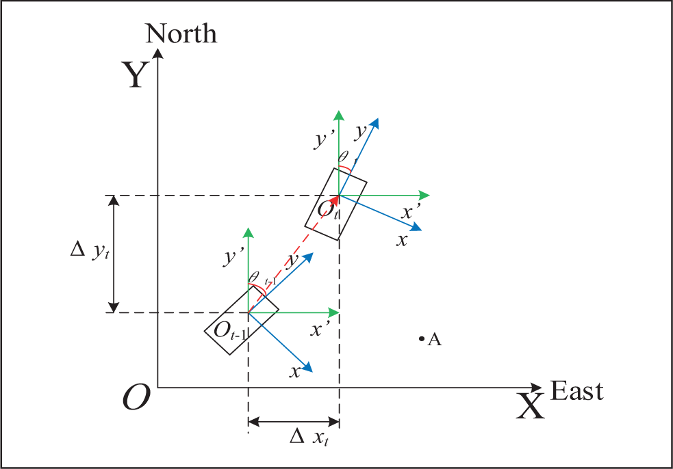
By using Charles’s method,¹⁷ the latitudes and longitudes parsed from real-time kinematic GPS (RTK-GPS) recording the position of autonomous vehicle at each frame are converted to geodetic coordinate system XOY. So, we can get the plane coordinates P_t which is the position where recording frame t, formulated as equation (1). The y-axis of geodetic coordinate system XOY always points to the north direction, and the x-axis always points to the east direction. The coordinate system origin O is the position where autonomous vehicle records the first RTK-GPS at the beginning, so we can get autonomous vehicle’s relative translational amount $Δ P_{t}$ which can be formulated as equation (2) in any two consecutive frames.

P = (x_{t}, y_{t}) (t = 1, 2, 3...)

Δ P_{t} = (Δ x_{t}, Δ y_{t})

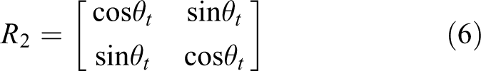
The x-axis of the bodywork’s coordinate system xoy points to the right of autonomous vehicle, and the y-axis points to the front of autonomous vehicle. The origin o is the center of HDL-64E LiDAR. Since the yaw angle data provided by autonomous vehicle’s inertial navigation system (INS) are not always the same, so we should consider the relationship of two frames’ yaw angles when we try to fuse the two consecutive frames. The point-cloud data of the static obstacle in the bodywork’s coordinate system $x o_{t - 1} y$ at previous frame are rotated to local bodywork’s coordinate system $x^{'} o_{t - 1} y^{'}$ whose x-axis and y-axis directions are the same like geodetic coordinate system XOY, and then the translation is carried out according to the relative translational amount $Δ P_{t}$ of the two frames. And finally, we should rotate the point-cloud data from coordinate system $x^{'} o_{t} y^{'}$ to the current bodywork’s coordinate system $x o_{t} y$ again, finishing two frames fusion.

Assuming that the autonomous vehicle’s yaw angle at previous frame t − 1 is $θ_{t - 1}$ , and the yaw angle at current frame t is $θ_{t}$ , which is defined as the clockwise angle between autonomous vehicle’s moving direction and the north direction. We pick up a point A whose coordinates are ( $x_{1}^{t - 1}$ , $y_{1}^{t - 1}$ ) at previous frame t − 1 to describe the two-frame fusion process. Point A belonging to static obstacle whose coordinates are ( $x_{1}^{t - 1}$ , $y_{1}^{t - 1}$ ) in bodywork’s coordinate system $x o_{t - 1} y$ at previous frame t − 1 is rotated and translated to the local bodywork’s coordinate system $x^{'} o_{t} y^{'}$ at current frame t, and its new coordinates ( $x_{2}^{t - 1}$ , $y_{2}^{t - 1}$ ) can be obtained by equation (3), where R ₁ is the rotation and translation matrix, defined as equation (4)

[x_{2}^{t - 1}, y_{2}^{t - 1},1] = [x_{1}^{t - 1}, y_{1}^{t - 1},1] R_{1}

R_{1} = [\begin{matrix} c o s θ_{t - 1} & s i n - θ_{t - 1} & 0 \\ s i n - θ_{t - 1} & c o s θ_{t - 1} & 0 \\ - Δ x_{t} & - Δ y_{t} & 1 \end{matrix}]

After the rotation and the translation, we get the point coordinates ( $x_{2}^{t - 1}$ , $y_{2}^{t - 1}$ ) in the local bodywork’s coordinate system $x^{'} o_{t} y^{'}$ , and then we should rotate the point to the current bodywork’s coordinate system $x o_{t} y$ at current frame t. The point coordinates ( $x_{1}^{t}$ , $y_{1}^{t}$ ) which are ( $x_{1}^{t - 1}$ , $y_{1}^{t - 1}$ ) at previous frame t − 1 can be obtained through equation (5), where R ₂ is the rotation matrix, defined as equation (6)

[x_{1}^{t}, y_{1}^{t}] = [x_{2}^{t - 1}, y_{2}^{t - 1}] R_{2}

R_{2} = [\begin{matrix} cos θ_{t} & sin θ_{t} \\ sin θ_{t} & cos θ_{t} \end{matrix}]

A single frame of point-cloud data contains about 130,000 points, so if all the points belonging to the static obstacle cells are rotated and translated, the calculation will be very large. Some static obstacle cells contain about thousands of points, after the rotation and translation, the points will still fall into the same cells. So we randomly select five points in each static obstacle cell (if the points in the cell are less than five, all the points are taken as calculation points) as the calculation points and the remaining points will be discarded. Six points, seven points, and even more points can be selected, but it depends on different computing platforms. The more the points in the cell are selected, the better the performance of multi-frame fusion is, but how many points should be selected depends on the need of ensuring the real-time performance of the algorithm on different computing platforms. The cells at current frame will be marked as static obstacle cells which the calculation points belonging to the static obstacle cells at previous frame fall into after the rotation and translation. On the basis of two-frame fusion, the coordinates of the static obstacle point-cloud data which was sampled at previous frame will have their new coordinates in the bodyworks coordinate system $x o_{t} y$ at current frame, so the multi-frame fusion can work out. We have fused six frames of point-cloud data through the method proposed by this article.

As the INS and HDL-64E LiDAR installation location on autonomous vehicle are not at the same place, the yaw angle data produced by INS belong to INS itself and do not belong to HDL-64E LiDAR. When autonomous vehicle conducts lateral control, the yaw angle we get from INS cannot represent the HDL-64E LiDAR’s yaw angle accurately. Therefore, if autonomous vehicle’s yaw angle changes greater than about 1.22 rad/s (demonstrated by large amount of experiments), the proposed multi-frame fusion method cannot operate well. Even so, in most scenarios of the city and almost all scenarios of the highway, the proposed method can perform well. Figure 6 shows the result of static obstacles detection; Figure 7(a) is the original point-cloud data after road segmentation in a single frame. The green part of Figure 7(b) is the static obstacle detection result in a single frame, and the green part of Figure 7(c) is the static obstacle detection result of multi-frame fusion. From Figure 7, the static obstacle detection result of multi-frame fusion is much better than in a single frame. The static obstacle detection method of multi-frame fusion can detect occluded static obstacles which are caused by moving obstacles and can also effectively retain the static obstacle detection results of history frames, such as box no.1 and area out of LiDAR detection range like box no.2, which will bring positive effect on the short period of autonomous vehicle path planning and decision-making.

Figure 6.

Static obstacle detection results (colored green) in a single frame.

Figure 7.

(a) Original point-cloud data after road segmentation in a single frame. (b) Static obstacle detection result in a single frame. (c) Static obstacle detection result of multi-frame fusion.

Moving obstacle detection and tracking

The purpose of moving obstacle detection and tracking is to obtain the movement state of the moving obstacle, so as to predict the possible state and trajectory of the moving obstacle, which is of great significance to path planning and decision-making of autonomous vehicle. In this article, a moving obstacle detection method based on the detected travelable area and feature templates matching is proposed. Data association is carried out on the basis, and moving obstacle is tracked by the improved dynamic tracking point model and Kalman filter.

Moving obstacle detection

The moving obstacle detection results achieved by geometric features matching algorithm^18,19 sometimes are prone to be false, so we use multi-frame fusion detection result of static obstacle to determine the travelable area, and then the moving obstacle which has been detected through the geometric features matching algorithm will be regarded as the real moving obstacles if they are located in the determined travelable area, and they will be tracked. Other moving obstacles which are not located in the determined travelable area detected by geometric features matching algorithm are regarded as normal obstacles, and we only deliver their location information to autonomous vehicle for path planning and decision-making without tracking it, which can largely avoid the occurrence of false detections.

First of all, we use the geometric features matching algorithm by Asma and Olivier¹⁹ to detect the majority of moving obstacles, as shown in Figure 8; the blobs which are colored black are moving obstacles in the primary detection step. But from the box no.1 in the left figure of Figure 8, using the geometric features matching algorithm is prone to have false detection, so we come up with the method of using travelable area to detect moving obstacles.

Figure 8.

Travelable area detection result.

Refer to Figure 9 when we determine the travelable area. Firstly, the longitudinal search is carried out dead ahead and dead astern from autonomous vehicle’s position O. When encountering the static obstacle cell, we stop the search and take cells A and B as the terminal cells. Then, we conduct lateral searches on both sides in accordance with the order from O to A and B, and the search will be terminated when encountering the static obstacle cell. If the offset distance between previous lateral search termination position and the current lateral search termination position is 4.5 m or more, it will be considered that we do not find a static obstacle cell, such as cell C, but if we encounter the normal obstacle cell, its position will be used as the lateral search termination position, such as cell D, otherwise we will use the last termination position as the current termination position. So we can easily determine the travelable area surrounded by the brown box in Figure 9. All the detected moving obstacles located in the travelable area are considered to be real moving obstacles. Figure 8 shows the detection result of travelable area. The red portion in the left picture of Figure 8 is detected as the travelable area, and the moving obstacles are bounded by red rectangles in the right figure.

Figure 9.

The diagram of detecting travelable area.

Data association of moving obstacle

For data association, we use the moving obstacle’s four boundaries’ position at current frame to calculate its similarities with other moving obstacles at previous frame. We define $M_{i}^{t}$ which contains four boundaries’ position of the ith obstacle at frame t as equation (7), where $i {Min}_{i}^{t}$ is cells’ minimum lateral index position of moving obstacle. $i {Max}_{i}^{t}$ is maximum lateral index position. $j {Min}_{i}^{t}$ is minimum longitudinal index position, and $j {Max}_{i}^{t}$ is maximum longitudinal index position.

M_{i}^{t} = (i {Min}_{i}^{t}, i {Max}_{i}^{t}, j {Min}_{i}^{t}, j {Max}_{i}^{t})

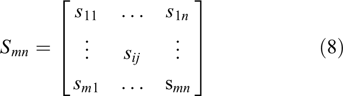
So we can get the similarity matrix $S_{m n}$ which is defined as equation (8) of all the moving obstacles between two consecutive frames, where m is the quantity of moving obstacles in the travelable area at previous frame, and n is the quantity of moving obstacles in the travelable area at current frame.

S_{m n} = [\begin{matrix} s_{11} & \dots & s_{1 n} \\ ⋮ & s_{i j} & ⋮ \\ s_{m 1} & \dots & s_{m n} \end{matrix}]

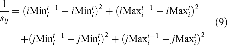
The similarity $s_{i j}$ which may belong to the same moving obstacle between two consecutive frames is defined as below

\begin{matrix} \frac{1}{s_{i j}} = (i {Min}_{i}^{t - 1} - i {Min}_{i}^{t})^{2} + {(i {Max}_{i}^{t - 1} - i {Max}_{i}^{t})}^{2} \\ + {(j {Min}_{i}^{t - 1} - j {Min}_{i}^{t})}^{2} + {(j {Max}_{i}^{t - 1} - j {Max}_{i}^{t})}^{2} \end{matrix}

The maximum $s_{i j}$ of each row may be the similarity which belongs to the same moving obstacle existing at both current frame and previous frame, and there are three conditions: (1) the moving obstacle at previous frame does exist at current frame, (2) the moving obstacle at previous frame is no longer present at current frame, and (3) a new moving obstacle is present at current frame, and the previous frame did not have this moving obstacle. Therefore, even if the similarity is the largest, it may not be the same moving obstacle, so by setting an appropriate threshold, we can distinguish whether the same moving obstacle exists at both previous frame and current frame. If similarity $s_{i j}$ is larger than threshold, we think that the moving obstacle does exist at two consecutive frames; otherwise the same moving obstacle doesn’t exist at two consecutive frames. We determined that the appropriate threshold is 0.005; 0.005 is the reasonable threshold based on large amount of online experiments and offline simulations.

Moving obstacle tracking

The selection of tracking point has a great impact on the tracking result of moving obstacle. When using HDL-64E LiDAR to track the moving obstacle, point-cloud data combined with the prior shape knowledge of the moving obstacle can deduce the moving obstacle’s center position,^20,21 but in fact, the shapes of all the moving obstacles do not strictly meet the specific models, and because of the obstacle’s occlusion and self-occlusion, the deduced center position cannot represent the vehicle’s position precisely. We improve Xiao et al.’s method,²² and when the moving obstacle is in different regions, different optimum tracking point is selected, and when the moving obstacle switches from a region to another region, the length and width of the moving obstacle are taken into account. We propose a new dynamic tracking point model to find the optimum tracking point of the moving obstacle. As shown in Figure 10, we divide the area around autonomous vehicle into eight different regions according to its relative position to autonomous vehicle.

When the moving obstacle is in A₃ and A₅, we should firstly find all the cells which are at the bottom of each cell column, and then find out the nearest point to autonomous vehicle from these cells as the tracking point which may be found in the red cell.

When the moving obstacle is in A₁, A₂, A₆, and A₇, we should firstly find all the cells which are at the top of each cell column and then find the nearest point to autonomous vehicle as the tracking point from the found cells.

When the moving obstacle is in A₄, we should firstly find all the cells which are at the bottom of each cell column, and when the moving obstacle is in A₈, we should firstly find all the cells which are at the top of each cell column and then take the nearest point in the rightmost cell as the tracking point.

When the moving obstacle switches from A₂ to A₃ and from A₆ to A₅, the obstacle’s length should be subtracted, and the obstacle’s length should be added when the moving obstacle switches from A₃ to A₂ and from A₅ to A₆. When the moving obstacle switches from A₄ to A₅ and from A₈ to A₇, the obstacle’s length should be subtracted. And when the moving obstacle switches from A₅ to A₄ and from A₇ to A₈, the obstacle’s length should be added. The length and width of the obstacle are calculated with the cells’ length and width at the time of switching, without relying on prior shape knowledge.

Figure 10.

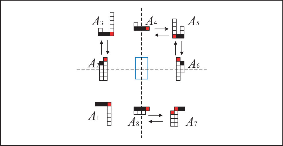
The diagram of dynamic tracking point model.

The movement state of the moving obstacle can be formulated as below

X = [X_{t}^{i}, Y_{t}^{i}, v_{t x}^{i}, v_{t y}^{i}]^{T}

Where

[\begin{matrix} v_{t x}^{i} \\ v_{t y}^{i} \end{matrix}] = [\begin{matrix} v_{t}^{i} sin θ_{t}^{i} \\ v_{t}^{i} cos θ_{t}^{i} \end{matrix}]

In equation (10), ( $X_{t}^{i}$ , $Y_{t}^{i}$ ) is the abscissa and ordinate of the ith moving obstacle in geodetic coordinate system XOY at frame t, and they can be obtained through equation (12). $v_{t x}^{i}$ and $v_{t y}^{i}$ are the moving obstacle’s eastward and northward component velocities, respectively. $v_{t}^{i}$ is the moving obstacle’s resultant velocity, and $θ_{t}^{i}$ is the moving obstacle’s yaw angle, defined as the clockwise angle between moving direction and north direction.

[X_{t}^{i}, Y_{t}^{i},1] = [x_{t}^{i}, y_{t}^{i},1] R_{3}

Where

R_{3} = [\begin{matrix} cos θ_{t}^{i} & sin - θ_{t}^{i} & 0 \\ sin - θ_{t}^{i} & cos θ_{t}^{i} & 0 \\ x_{t} & y_{t} & 1 \end{matrix}]

( $x_{t}^{i}$ , $y_{t}^{i}$ ) is the tracking point’s coordinates of the ith moving obstacle at frame t in bodywork’s coordinate system $x o_{t} y$ , and (x_t,y_t) of matrix R ₃ is autonomous vehicle’s coordinates in geodetic coordinate system XOY at frame t.

Assuming that the coordinates of the ith moving obstacle at frame t − 1 is ( $x_{t - 1}^{i}$ , $y_{t - 1}^{i}$ ), the moving obstacle’s resultant velocity $v_{t}^{i}$ can be obtained by equation (14), where T is the time interval of two consecutive frames, and the value of T is 0.1 s, as the sampling frequency of HDL-64E LiDAR and GPS is 10 Hz.

v_{t}^{i} = \frac{\sqrt{{(x_{t}^{i} - x_{t - 1}^{i})}^{2} + {(y_{t}^{i} - y_{t - 1}^{i})}^{2}}}{T}

The yaw angle $θ_{t}^{i}$ of the moving obstacle is obtained by substituting equation (15) into equation (16)

{\begin{array}{l} Δ x_{t}^{i} = x_{t}^{i} - x_{t - 1}^{i} & ​ \\ Δ y_{t}^{i} = y_{t}^{i} - y_{t - 1}^{i} & ​ \end{array}

θ_{t}^{i} = {\begin{array}{l} arctan \frac{Δ x_{t}^{i}}{Δ y_{t}^{i}} \times \frac{180}{π} & Δ x_{t}^{i} \geq 0, Δ y_{t}^{i} > 0 \\ arctan - \frac{Δ y_{t}^{i}}{Δ x_{t}^{i}} \times \frac{180}{π} + 90 & Δ x_{t}^{i} > 0, Δ y_{t}^{i} \leq 0 \\ arctan \frac{Δ x_{t}^{i}}{Δ y_{t}^{i}} \times \frac{180}{π} + 180 & Δ x_{t}^{i} \leq 0, Δ y_{t}^{i} < 0 \\ arctan - \frac{Δ y_{t}^{i}}{Δ x_{t}^{i}} \times \frac{180}{π} + 270 & Δ x_{t}^{i} < 0, Δ y_{t}^{i} \geq 0 \\ 0 & Δ x_{t}^{i} = 0, Δ y_{t}^{i} = 0 \end{array}

The system state equation and measurement equation can be expressed as equation (17) at time k. $A$ is the state transition matrix which is defined as equation (18), and $H$ is the observation matrix which is defined as equation (19). $w_{k - 1}$ is the system noise vector and v_k is the observation noise vector. We substitute the above state matrixes and vectors into the standard Kalman filter.²³

{\begin{array}{l} X_{k} = A X_{k - 1} + w_{k - 1} \\ Z_{k} = H X_{k} + v_{k} \end{array}

A = [\begin{matrix} 1 & 0 & T & 0 \\ 0 & 1 & 0 & T \\ 0 & 0 & 1 & 0 \\ 0 & 0 & 0 & 1 \end{matrix}]

H = [\begin{matrix} 1 & 0 & 0 & 0 \\ 0 & 1 & 0 & 0 \\ 0 & 0 & 1 & 0 \\ 0 & 0 & 0 & 1 \end{matrix}]

${\hat{X}}_{k + 1 | k}$ is the prediction vector of ${\hat{X}}_{k}$ at time k + 1 and can be obtained by the following equation

{\hat{X}}_{k + 1 | k} = A {\hat{X}}_{k}

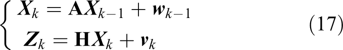
The optimal estimation ${\hat{X}}_{k + 1}$ at time k + 1 can be obtained through equation (21), where $K_{k + 1}$ is the Kalman gain which can be obtained through equation (22) at time k + 1, and $Z_{k + 1}$ is the actual observation of moving obstacle at time k + 1.

{\hat{X}}_{k + 1} = {\hat{X}}_{k + 1 | k} + K_{k + 1} (Z_{k + 1} - H {\hat{X}}_{k + 1 | k})

K_{k + 1} = P_{k + 1 | k} H^{T} {(H P_{k + 1 | k} H^{T} + R)}^{(- 1)}

$P_{k + 1 | k}$ is the prediction covariance matrix, which can be obtained through equation (23), and the observation noise matrix R is defined as Gaussian white noise diagonal matrix with the mean value of 0 m and standard deviation of 1 m with positive values. The state transition noise matrix Q is defined as Gaussian white noise diagonal matrix with the mean value of 0 m and standard deviation of 0.5 m with positive values.

P_{k + 1 | k} = A P_{k} A^{T} + Q

After the optimal estimation of ${\hat{X}}_{k + 1}$ , it is necessary to update $P_{k}$ to $P_{k + 1}$ through equation (24). Through the process mentioned above, the Kalman filter can work it out, getting the stable tracking result of moving obstacle.

P_{k + 1} = (I - K_{k + 1} H) P_{k + 1 | k}

Experimental results and analysis

Our experimental vehicle is JJUV-5, the champion of 2016 China Intelligent Vehicle Future Challenge (see Figure 11). The main sensors include a velodyne HDL-64E LiDAR, a set of RTK-GPS system, and an Inertial + INS, and the computer is equipped with Intel quad-core i5-3350p processor.

Figure 11.

JJUV-5 autonomous vehicle.

The experiment is carried out in a city scenario, which includes static obstacles such as roadside, buildings, stationary vehicles, and other moving obstacles such as bicycles and moving cars. Table 1 is the detection result of the proposed approach. The roadside detection rate is calculated by dividing all the frames by the quantity of frames in which roadside are successfully detected, and the false detection rate is calculated by dividing all the frames by the quantity of frames in which obstacles are wrongly detected as roadside. The moving obstacle detection rate is calculated by dividing the quantity of actual moving obstacles in all frames by the quantity of moving obstacles detected in all frames. And the false detection rate is calculated by dividing the quantity of moving obstacles detected in all frames by the quantity of obstacles wrongly detected as moving obstacles in all frames.

Table 1.

Detection result of the methods.

	Detection rate (%)	False detection rate (%)
Roadside	100	0.21
Moving obstacle (ours)	63.47	0.43
Moving obstacle (by Asma and Olivier¹⁹)	65.8	6.82

To further compare our approach, we also conduct the obstacle detection experiment presented by Asma and Olivier.¹⁹ The objective of this experiment is to estimate the obstacle detection rate and false detection rate of the proposed method in this article and the method by Asma and Olivier.¹⁹ Figure 12 shows that the proposed method in this article can robustly detect static obstacles as purple blobs and moving obstacles as black blobs. However, by using the method by Asma and Olivier,¹⁹ it leans to detect static obstacles which are colored purple as moving obstacles which are colored black in the left picture of Figure 12. So, it can be seen from parts 1 and 2 of Figure 12 that our method outperforms the method by Asma and Olivier.¹⁹ In Table 1, we report detection rate and false detection rate of moving obstacle by using the proposed method and the method by Asma and Olivier,¹⁹ and the results show that the method proposed in this article has lower false detection rate of moving obstacles than the method by Asma and Olivier.¹⁹

Figure 12.

The diagram of obstacle detection.

Because of the well-performed road segmentation algorithm and static obstacle detection of multi-frame fusion method, the static obstacle detection result is improved obviously. As the moving obstacles are detected based on the travelable area, the obstacles in the reverse lane are not detected as moving obstacles. The approach of handling the moving obstacle in the reverse lane is reasonable, because the moving obstacles in the reverse lane are not going to cross the fence into the lane where autonomous vehicle works, and providing its location to autonomous vehicle for path planning and decision-making is enough. The main factors which affect autonomous vehicle’s overtaking cars, following cars, changing lanes, and other actions are more from the moving obstacles which are located in the lane where autonomous vehicle works. Because the valid detection range of 3-D LiDAR is about 120 m and the density of point clouds decreases as the distance grows longer, it is difficult to detect moving obstacle when the obstacle is far away from 3-D LiDAR, and it is easier to have false detection when the distance is longer. When it comes to static obstacles false detection, there are always big trucks whose size are very long and wide running on the streets, the proposed algorithm inclines to detect the very long trucks as roadside. These are the main sources of obstacles false detection.

Figure 13 is the result of using the proposed approach to continuously track the three moving obstacles in 350 frames. Figure 14 shows the velocity and yaw angle obtained by using the proposed approach and the method by Xiao et al.²²

Figure 13.

The continuous tracking results of multi-frame in 350 frames. The blue box represents the position of autonomous vehicle, and other colored obstacles which are not colored black are detected moving obstacles. The frame of each figure is numbered as follows: (a) Frame 1. (b) Frame 18. (c) Frame 48. (d) Frame 80. (e) Frame 105. (f) Frame 110. (g) Frame 120. (h) Frame 150. (i) Frame 170. (j) Frame 201. (k) Frame 230. (l) Frame 300.

Figure 14.

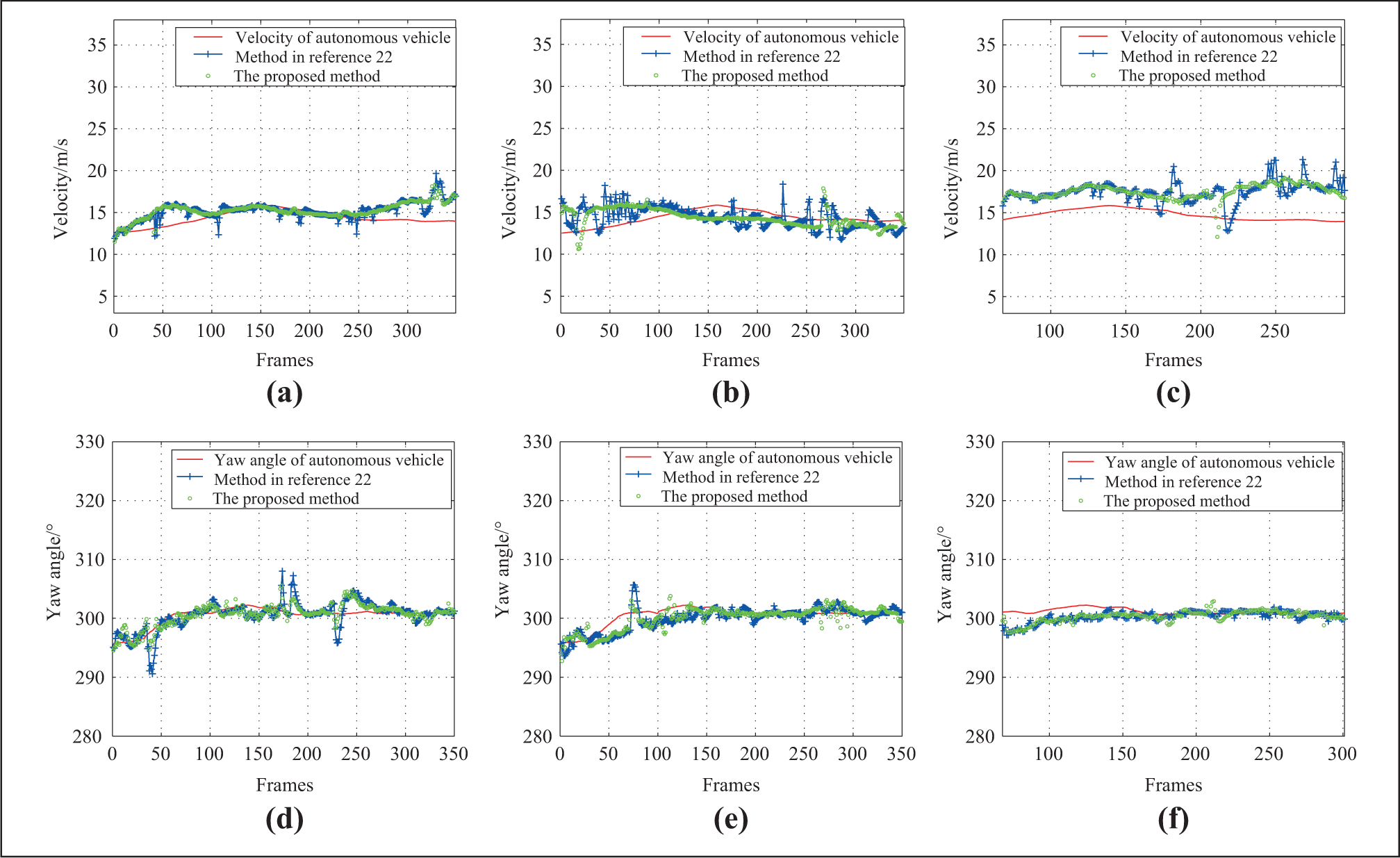
Tracking results of three dynamic obstacles’ yaw angle and velocity. (a) The velocity of obstacle No.1. (b) The velocity of obstacle No.2. (c) The velocity of obstacle No.3. (d) The yaw angle of obstacle No.1. (e) The yaw angle of obstacle No.2. (f) The yaw angle of obstacle No.3.

According to Figure 13, the proposed approach can continuously track the same moving obstacle whose color and number remain unchanged, such as the green obstacle which is marked “No.0” by the program. (obstacle 1 in this article). Obstacle 1 keeps green and the same number all the time in continuous 350 frames, which indicates that the proposed approach can robustly track the same obstacle. In addition, even when there are more moving obstacles, the proposed approach can still robustly track the various obstacles, as shown in Figure 13(a) to (c). Meanwhile, the static obstacles and moving obstacles which are not in the travelable area are black in one frame, indicating that the proposed approach can distinguish the static obstacles, moving obstacles which are not in the travelable and the moving obstacles needed to be tracked clearly. When tracking the moving obstacle 1 at the beginning, obstacle 1 is far away from the autonomous vehicle. And during this period from (a) to (d) of Figure 13, obstacle 1 keeps getting closer to the autonomous vehicle, as shown in Figure 14(a), and the velocity of obstacle 1 is obviously faster than the velocity of the autonomous vehicle. During the period from (e) to (k) of Figure 13, the distance between the obstacle 1 and the autonomous vehicle is almost constant. So in Figure 14(a), the velocity of the autonomous vehicle is almost equal to the velocity of obstacle 1. Then, during the period from (i) to (k) of Figure 13, it can be seen that obstacle 1 gradually approaches the autonomous vehicle and finally overtakes the autonomous vehicle. So, the velocity of obstacle 1 is faster than the velocity of the autonomous vehicle in Figure 14. The velocity of other obstacles like obstacle 2 which is marked “No.1” by the program and obstacle 3 which is marked “No.74” by the program is also in accordance with changes of position in Figure 13. It can be concluded that the proposed approach is robust in the process of tracking the moving obstacle and can obtain the accurate and stable velocity of the moving obstacle. So, when it comes to the complex urban scenarios and highway scenarios, the proposed approach has a very good applicability.

When the moving obstacle overtakes and changes lane, its yaw angle will change, so we can see little change of yaw angle in (d) and (e) of Figure 14. From Figure 13(d) to (m), it can be seen that the obstacle 3 has no lane change during the whole process, so that the yaw angle is stable in Figure 14(f). In this article, the average time-consuming of detecting and tracking at each frame is 96.085 ms during 350 frames, which satisfies the real-time perception requirement of autonomous vehicle.

Conclusions

In this article, we present an approach for detecting and tracking obstacles in 3-D LiDAR point clouds. Firstly, the point clouds produced by 3-D LiDAR after the road segmentation are rasterized, and additional useful cells are added. Then, the proposed clustering algorithm clusters the obstacle cells efficiently. Based on the clustering result, static obstacles are detected by the proposed multi-frame fusion method, and moving obstacles located in the travelable area are further detected. Lastly, the improved dynamic tracking point model and standard Kalman filter are used to track the moving obstacles, obtaining the stable movement state. The reliability of the proposed approach is demonstrated in various challenging scenarios. The autonomous vehicle developed by us can percept its surrounding environment well by using the proposed approach, and we got the champions in 2015 and 2016 China Intelligent Vehicle Future Challenge. We believe that the proposed approach can help other developers detect and track obstacles accurately when using 3-D LiDAR.

The proposed approach has not yet been able to deal with the situations in which the obstacles are very close to others, for example, vehicles very closed to the roadside will be clustered into one blob with the roadside. We will establish a variable scale occupancy grid map in which the cells’ size near autonomous vehicle is 10 cm × 10 cm, and in the long distance is 40 cm × 40 cm to deal with the situation that the point clouds near autonomous vehicle are denser than the point clouds in the distance. At the same time, we will focus on HDL-64E and GPS/INS calibration work to improve the real-time static obstacle detection of multi-frame fusion. The GPS data received on the streets can be influenced by building occlusions, making the GPS data less accurate. But by using our developed localization algorithm which fuses GPS raw data, INS data, point clouds, and vision data from camera, the GPS localization precision can be improved to some extent, but it is difficult to keep GPS accurate all the time when the autonomous vehicle drives itself on the streets, so we will further improve our localization algorithm to make the proposed algorithm more applicable.

Footnotes

Declaration of conflicting interests

The author(s) declared no potential conflicts of interest with respect to the research, authorship, and/or publication of this article.

Funding

The author(s) disclosed receipt of the following financial support for the research, authorship, and/or publication of this article: This work is supported by National Natural Science Foundation of China (Grant No. 91220301) and 973 Program of China (Grant No. 2016YFB0100903).

ORCID iD

Desheng Xie

References

Ratan

Clint

Garrett

. Self-driving cars. San Francisco: College of Engineering University of California, Berkeley, 2013.

Acharya

Lee

Chen

. Real time car detection and tracking in mobile devices. In: 2012 international conference on connected vehicles and expo, 12–16 December 2012, pp. 239–240. IEEE. http://ieeexplore.ieee.org/document/6519578/ (accessed 27 May 2013).

Leissi

Roberto

. Car detection in sequences of images of urban environments using mixture of deformable part models. Pattern Recognit Lett 2014; 39: 39–51.

Julius

Philipp

Markus

. Making bertha drive-an autonomous journey on a historic route. IEEE Int Trans Syst Magaz 2014; 6(2): 108–120.

Ayush

Tim

Gian

. Motion-based detection and tracking in 3D LiDAR scans. In: 2016 IEEE International conference on robotics and automation (ICRA), Stockholm, Sweden, 16–21 May 2016, pp. 4508–4513. IEEE. http://ieeexplore.ieee.org/document/7487649/ (accessed 9 June 2016).

Qiaohui

Bin

Hao

. LiDAR-based dynamic environment modeling and tracking using particles based occupancy cell. In: Proceedings of 2016 IEEE International conference on mechatronics and automation, 7–10 August 2016, pp. 238–243. IEEE. http://ieeexplore.ieee.org/document/7558567/ (accessed 5 September 2016).

Alireza

Cristiano

Paulo

. 3D LiDAR-based static and moving obstacle detection in driving environments: An approach based on voxels and multi-region ground planes. Robot Auto Syst 2016; 83: 299–311.

Keyu

Xiangjing

Jian

. Efficient deep network for vision-based object detection in robotic applications. Neurocomputing 2017; 245(C): 31–45.

Wen

Jing

Mao

. Real-time target detection and recognition with deep convolutional networks for intelligent visual surveillance. In: 2016 IEEE/ACM 9th International conference on utility and cloud computing, Shanghai, China, 6–9 December 2016, pp. 321–326. IEEE. http://ieeexplore.ieee.org/document/7881652/ (accessed 20 March 2017).

10.

Yang

. Moving objects real-time detection and tracking based on 3D LiDAR. Hangzhou: Zhejiang University, 2012.

11.

Xin

Liang

Mei

. Dynamic obstacle detection and representation approach for unmanned vehicles based on laser sensor. Robot 2014; 36(6): 654–661.

12.

Himmelsbach

Wuensche

. Tracking and classification of arbitrary objects with bottom-up/top-down detection. In: 2012 Intelligent vehicles symposium, Alcala de Henares, Spain, 3–7 June 2012, pp. 577–582. IEEE. http://ieeexplore.ieee.org/document/6232181/ (accessed 5 July 2012).

13.

Ralf

Jérôme

Yves

. Generative object detection and tracking in 3D range data. In: 2012 IEEE international conference on robotics and automation, 14–18 May 2012, pp. 3075–3081. IEEE. http://ieeexplore.ieee.org/document/6224585/ (accessed 28 June 2012).

14.

Frank

Christoph

. Joint self-localization and tracking of generic objects in 3D range data. In: 2013 IEEE International conference on robotics and automation (ICRA), Karlsruhe, Germany, 6–10 May 2013, pp. 1146–1152. IEEE. http://ieeexplore.ieee.org/document/6630716/ (accessed 17 October 2013).

15.

Anna

Sebastian

. Model based vehicle detection and tracking for autonomous urban driving. Auto Robot 2009; 26(2–3): 123–139.

16.

Zhiyuan

Youchun

Yongle

. Vehicle targets detection method based on 3D LiDAR. J Military Transport University 2017; 19(1): 45–49.

17.

Charles

FFK

. Geodesics on an ellipsoid of revolution. Princeton: SRI International, 2011. http://geographiclib.sourceforge.net/geod.html (accessed 30 September 2017).

18.

Jang

Yoon

Kim

. Research of object classification algorithm based on LiDAR for UGV. In: 2011 11th International conference on control, automation and systems, 26–29 October 2011, pp. 746–749. IEEE. http://ieeexplore.ieee.org/document/6106291/ (accessed 19 December 2011).

19.

Asma

Olivier

. Detection, classification and tracking of moving objects in a 3D environment. In: 2012 Intelligent vehicles symposium, Alcala de Henares, Spain, 3–7 June 2012, pp. 802–807. IEEE. http://ieeexplore.ieee.org/document/6232303/ (accessed 5 July 2012).

20.

Rulin

Huawei

Jiajia

. LiDAR based dynamic obstacle detection, tracking and recognition method for driverless cars. Robot 2016; 38(4): 437–443.

21.

Fortin

Noyer

Lherbier

. A particle filtering approach for joint vehicular detection and tracking in LiDAR data. In: International instrumentation and measurement technology conference proceedings, Graz, Austria, 13–16 May 2012, pp. 391–396. IEEE. http://ieeexplore.ieee.org/document/6229413/ (accessed 2 July 2012).

22.

Xiao

Keqiang

Jianqiang

. Parameter identification of intelligent vehicle target based on 3D laser rada. Auto Eng 2016; 38(9): 1146–1152.

23.

João

VFN

Jorge

José

APdA

. QR-duality tuning of standard Kalman filter oriented to rocket velocity indirect measurement. In: 2010 12th International conference on computer modelling and simulation, Cambridge, UK, 24–26 March 2010, pp. 74–79. IEEE. http://ieeexplore.ieee.org/document/5480263/ (accessed 7 June 2010).