Sage Journals: Discover world-class research

Abstract

A novel control approach is proposed for trajectory tracking of a wheeled mobile robot with unknown wheels’ slipping. The longitudinal and lateral slipping are considered and processed as three time-varying parameters. The adaptive unscented Kalman filter is then designed to estimate the slipping parameters online, an adaptive adjustment of the noise covariances in the estimation process is implemented using a technique of covariance matching in the adaptive unscented Kalman filter context. Considering the practical physical constrains, a stable tracking control law for this robot system is proposed by the backstepping method. Asymptotic stability is guaranteed by Lyapunov stability theory. Control gains are determined online by applying pole placement method. Simulation and real experiment results show the effectiveness and robustness of the proposed control method.

Keywords

Adaptive unscented Kalman filter unknown wheels’ slipping pole placement method tracking control wheeled mobile robot

Introduction

Over the last several years, the control problem of the wheeled mobile robot (WMR) has been regarded as a fascinating problem because of the property of its nonholonomic constraints. Many developed controllers have been designed for tracking and stabilization of nonholonomic mobile robots using several nonlinear control techniques such as sliding mode control,^1–6 adaptive control,^7–11 backstepping control^12
–14 and intelligent control based on neural networks,^15

–19 fuzzy control,^20–23 and other intelligent control method.^24,25

The previous papers^1–24 assume nonholonomic constraints for the controlled WMR. The nonholonomic constraints are generated by the assumption that the mobile robots are subject to a “pure rolling without slipping.” However, since the robotic wheels’ slipping can happen in various practical environments such as the on wet or icy roads, rough terrain, or the rapid cornering, the nonholonomic constraint can be disturbed in a few literatures.^26

–29 To deal with this case, control methods for mobile robots considering slipping were proposed in a few literatures.^26–35 Wang and Low³² proposed models of the WMR with wheels’ slipping and examined their controllability according to the outdoor maneuverability of the WMR. Moreover, they presented control approaches for trajectory tracking of mobile robots considering skidding and slipping.^31,32 However, the information of skidding and slipping is measured by the global positioning system and small initial conditions between the actual robot and the reference robot are required to design the controllers in.^31,32 Additionally, these papers^33,34 only considered the longitudinal slipping of the kinematic model for mobile robots without lateral slipping. The study by Zhou et al.³⁵ only considered the lateral slipping of the kinematic model for the WMR without longitudinal slipping. The papers by Cui et al. (2014), Tian and Sarkar (2014), and Yoo (2011)^26
–28 are excellent and distinguished works to deal with slipping perturbation; however, practical physical control constrains are not considered in the process of controller design.

Accordingly, the main theory contributions of our work are the design of an adaptive controller for tracking trajectory the WMR with unknown wheels’ slipping at the kinematics level. More specifically, in the theoretical aspect of this article, considering practical physical constrains, we design a control law that guarantees tracking with bounded error for the WMR with unknown slipping. First, the kinematic model of the WMR considering the slipping is induced from nonholonomic constraints. Three slipping parameters are estimated online by the adaptive unscented Kalman filter (AUKF). An adaptive adjustment of the noise covariances in the estimation process is implemented using a technique of covariance matching in the AUKF context. Meanwhile, a stable tracking control law for this nonholonomic system is proposed and the asymptotic stability is guaranteed by Lyapunov theory. From the Lyapunov stability theorem, we prove that tracking errors of the controlled closed-loop system are uniformly bounded and the tracking errors can be made arbitrarily small by adjusting design parameters regardless of large initial tracking errors and unknown slipping. Second, to simplify the complexity of the tuning parameters for the proposed controller, the controller gains are computed using pole placement method. To the best of our knowledge, this is the first design of a tracking controller for the WMR with two independently driving wheels. Finally, we provide simulation results to verify the effectiveness of the proposed controller.

This article is organized as follows. In “Kinematic model of the WMR with wheels’ slipping” section, we present the kinematics model of WMRs with longitudinal and lateral slipping induced from nonholonomic constraints. In “A scheme of the robotic slipping parameter estimation” section, an AUKF is employed to estimate three unknown sliding parameters. In “A scheme of the robotic slipping parameter estimation” section, a tracking controller for mobile robots in the presence of unknown longitudinal and lateral slipping is designed, and the stability of the proposed control system is analyzed. In “Adaptive adjustment of control parameters” section, a method of adjusting the control parameters online is proposed. Simulation results are discussed in “Simulations and experiment” section. Finally, “Conclusions” section gives some conclusions.

Kinematic model of the WMR with wheels’ slipping

A scheme of the WMR is shown as Figure 1. The two front wheels are driven independently by two direct current servo motors, respectively. The two rear wheels are supporting rollers, and they only play the roles of supporting car body, but no guidance.

Figure 1.

WMR with two independent driving wheels. WMR: wheeled mobile robot.

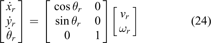
To describe the motion features of tracked WMR simply and rigorously in the general plane motion, a fixed reference coordinate frame F₁(x_w, y_w) and a moving coordinate frame F₂(x_m, y_m) are defined which attach to the robot body with origin at the geometric center O_m . ω is the angular velocity of the WMR around the geometric center O_m .

The linear velocities of left and right driving wheels of mobile robot without slipping are given as follows

\begin{matrix} v_{L} = r ω_{L} \\ v_{R} = r ω_{R} \end{matrix}

where ω_L and ω_R are the angular velocities of the left and right wheels, respectively and r is radius of the wheels. Longitudinal slipping ratio of the left and right wheels of the WMR are defined as follows³³

\begin{matrix} a_{L} = \frac{r ω_{L} - v_{L}^{s}}{r ω_{L}} \\ a_{R} = \frac{r ω_{R} - v_{R}^{s}}{r ω_{R}} \end{matrix}

where $v_{L}^{s}$ and $v_{R}^{s}$ are the relative to the ground linear velocities of the left and right wheels of the WMR with wheels’ slipping, respectively.

Assumption 1

The range of longitudinal slip ratio $a_{L}, a_{R} \in (- \infty, 1) \cup (1, + \infty)$ .

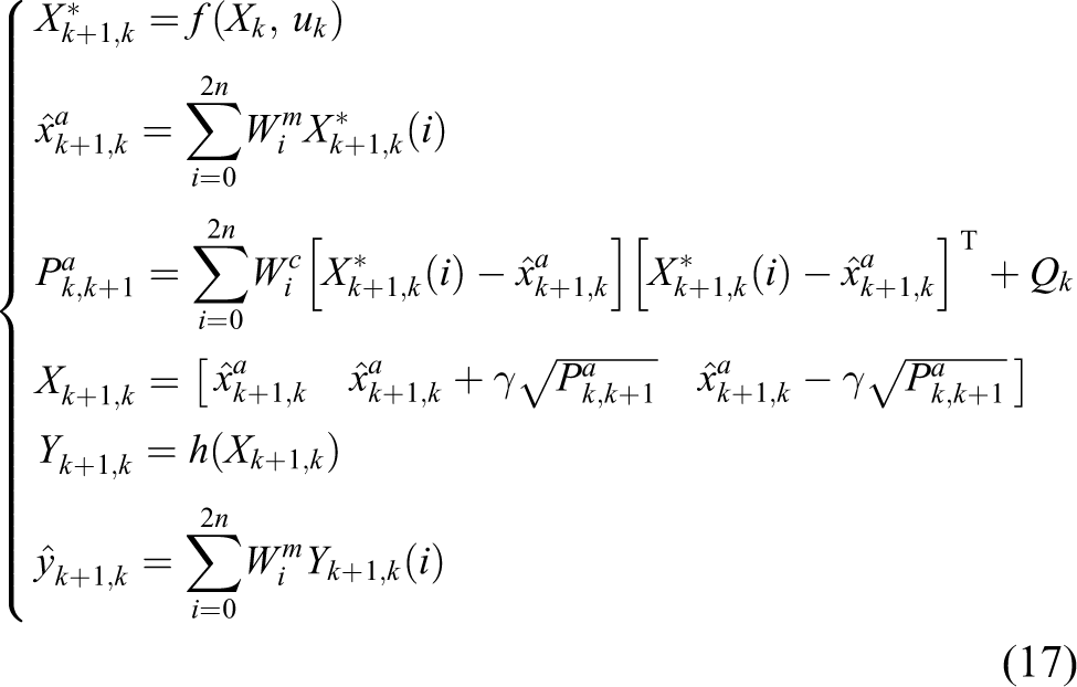
Remark 1

If a_R = a_L = 1, from equation (2), we know that $v_{L}^{s} = v_{R}^{s} = 0$ , it implies a complete slipping, that is, the wheels of the mobile robot are rotating, while its forward speed is zero, the mobile robot is uncontrollable, this case is not considered. When $v_{L}^{s} > r ω_{L}$ or $v_{R}^{s} > r ω_{R}$ , that is, a_R < 0 or a_L < 0, it indicates decelerated slipping (such as braking process).

Lateral slipping ratio of the WMR is defined as³⁵

$δ = tan α$
3

where α is the lateral slipping angle of a mobile robot (see Figure 1), it is the angle between the velocity of the mobile robot v and the x axis of a local frame attached to the mobile robot.

Assumption 2

The lateral slip angle α lies in (0, π/2).

Remark 2

If α = π/2, it implies that mobile robot is in a state of complete lateral slipping, the mobile robot is uncontrollable, this case is not considered. That is, lateral slip ratio δ is bounded.

From equation (2), the linear velocities of the left and right wheels of the mobile robot with wheels’ slipping are given as

$\begin{array}{l} v_{L}^{s} = r ω_{L} (1 - a_{L}) \\ v_{R}^{s} = r ω_{R} (1 - a_{R}) \end{array}$
4

In coordinate frame F₁(x_w, y_w), the kinematic mode of the WMR without wheels’ slipping is described as

$[\begin{matrix} \dot{x} \\ \dot{y} \\ \dot{θ} \end{matrix}] = [\begin{matrix} \cos θ & 0 \\ sin θ & 0 \\ 0 & 1 \end{matrix}] [\begin{matrix} v \\ ω \end{matrix}]$
5

In coordinate frame F₂(x_m, y_m), a suitable model with slipping can be written as

$\begin{array}{l} {\dot{x}}_{m} = \frac{r ω_{L} (1 - a_{L}) + r ω_{R} (1 - a_{R})}{2} \\ {\dot{y}}_{m} = - \frac{r ω_{L} (1 - a_{L}) + r ω_{R} (1 - a_{R})}{2} δ \\ \dot{θ} = \frac{r ω_{R} (1 - a_{R}) - r ω_{L} (1 - a_{L})}{b} \end{array}$
6

where b is the distance between two driving wheels. As shown in Figure 1, the coordinate rotation transformation from F₂(x_m, y_m) to F₁(x_w, y_w) is given by

$[\begin{matrix} x \\ y \end{matrix}] = [\begin{matrix} \cos θ & - sin θ \\ sin θ & \cos θ \end{matrix}] [\begin{matrix} x_{m} \\ y_{m} \end{matrix}]$
7

From equations (6) and (7), in coordinate frame F₁(x_w, y_w), the kinematic mode of the differential WMR with slipping is described as follows

$\begin{array}{l} \dot{x} = \frac{r ω_{L} (1 - a_{L}) + r ω_{R} (1 - a_{R})}{2} (\cos θ + δ sin θ) \\ \dot{y} = \frac{r ω_{L} (1 - a_{L}) + r ω_{R} (1 - a_{R})}{2} (sin θ - δ cos θ) \\ \dot{θ} = \frac{r ω_{R} (1 - a_{R}) - r ω_{L} (1 - a_{L})}{b} \end{array}$
8

where [x, y, θ] ^T is posture vector of the mobile robot and θ is heading angle of the WMR.

Assumption 3

Slipping parameters a_R , a_L , and δ are not measurable.

Define an auxiliary control input [v, ω] ^T , and then the relationship between auxiliary control input and real control input [ω_L, ω_R] ^T is regarded as

$[\begin{matrix} v \\ ω \end{matrix}] = [\begin{matrix} \frac{r (1 - a_{L}) ω_{L} + r (1 - a_{R}) ω_{R}}{2} \\ \frac{- r (1 - a_{L}) ω_{L} + r (1 - a_{R}) ω_{R}}{b} \end{matrix}] = T [\begin{matrix} ω_{L} \\ ω_{R} \end{matrix}]$
9

where matrix $T = r [\begin{matrix} \frac{1 - a_{L}}{2} & \frac{1 - a_{R}}{2} \\ \frac{- (1 - a_{L})}{b} & \frac{1 - a_{R}}{b} \end{matrix}]$ , T is a nonsingular matrix. From equation (9), virtual control input [ω_L, ω_R] ^T can be obtained as follows

$[\begin{matrix} ω_{L} \\ ω_{R} \end{matrix}] = T^{- 1} [\begin{matrix} v \\ ω \end{matrix}] = \frac{1}{r} [\begin{matrix} \frac{1}{1 - a_{L}} & - \frac{b}{2 (1 - a_{L})} \\ \frac{1}{1 - a_{R}} & \frac{b}{2 (1 - a_{R})} \end{matrix}] [\begin{matrix} v \\ ω \end{matrix}]$
10

Then, equation (8) can be rewritten as

$[\begin{matrix} \dot{x} \\ \dot{y} \\ \dot{θ} \end{matrix}] = [\begin{matrix} \cos θ + δ sin θ & 0 \\ sin θ - δ cos θ & 0 \\ 0 & 1 \end{matrix}] [\begin{matrix} v \\ ω \end{matrix}]$
11

We can see from equation (8), to handle tracking control problem of the WMR with unknown slipping parameters a_L , a_R , and δ, it is the top priority to estimate time-varying slipping parameters online, and then to design tracking controller on the basis of the estimation of the slipping parameters.

A scheme of the robotic slipping parameter estimation

Because three slipping parameters a_R , a_L , and δ in equation (8) cannot be measured directly, it is necessary to estimate slipping parameters in order to design tracking controller. To estimate the states and slipping parameters, joint estimation technique can be used, that is, states and parameters are estimated simultaneously using a same filter.³⁶ It is often used to solve the state feedback control with uncertain parameters, or the modeling of the parameters with noise and states that can’t be measured directly. Because of the incorporation of the states and the parameters, more accurate results may be made using this approach. In the localization of the WMR with slipping, the pose and the slipping parameters should be estimated at the same time. A new state vector P = [x, y, θ, a_R, a_L, δ] ^T is defined as a combination of the old states and parametric vector. In this augmented state, the dynamic of the slipping parameters are often unknown. In discrete time domain, it can be rewritten as following

$P_{k + 1} = P_{k} + w_{p, k}, k = 0, 1, 2, …$
12

where P_k ∈ R_p is the discrete parametric vector and w_p,k ∈ R_p is the additive process noise which drives the model. The UKF is introduced to estimate jointly the state and slipping parameters. Unlike extended Kalman filter (EKF),³⁷ the UKF is able to approximate the nonlinear process and observation models.³⁸ Instead, it uses the true nonlinear models and approximates the distribution of the state random variable. The UKF, which does not need to compute the Jacobian, the so-called unscented transform and sigma points are used to propagate all of them through models. As a result, the UKF often leads to more accurate estimations than the EKF.

Given the following general nonlinear system

${\begin{cases} x_{k + 1} = f (x_{k}, u_{k}) + w_{k} \\ y_{k + 1} = h (x_{k}) + v_{k} \end{cases}$
13

where f(x_k, u_k) and h (x_k) are the nonlinear process and measurement models of the robot, respectively. The immeasurable state vector is represented by x_k = [x, y, θ, a_R, a_L, δ] _T , u_k is known as the control input vector, and $y_{k} = {[\dot{x}, \dot{y}, \dot{θ}]}^{T}$ is the observed output. w_k and v_k are process and measurement noise sequences with covariance Q_k and R_k , respectively. The initial state vector is defined as x ₀. The UKF algorithm is given as follows:³⁸

Standard UKF

Initization at k = 0

${\begin{cases} {\bar{x}}_{0} = E [x_{0}] \\ P_{0} = E [(x_{0} - {\bar{x}}_{0}) {(x_{0} - {\bar{x}}_{0})}^{T}] \end{cases}$
14

where ${\bar{x}}_{0}$ is the expected value of the initial state and P ₀ is initial covariance.

The augmented state including original states, parameters, and process noises are defined as

${\begin{cases} {\hat{x}}_{0}^{a} = {[{\bar{x}}_{0}^{T} 0 0]}^{T} \\ P_{0}^{a} = d i a g (P_{0}, Q_{0}, R_{0}) \end{cases}$
15

(2) For K=1,2,…,∞

(a) Calculate sigma points

$X_{k} = [\begin{matrix} {\hat{x}}_{k}^{a} & {\hat{x}}_{k}^{a} + γ \sqrt{P_{k}^{a}} & {\hat{x}}_{k}^{a} - γ \sqrt{P_{k}^{a}} \end{matrix}]$
16

(b) The prediction step

${\begin{cases} X_{k + 1, k}^{} = f (X_{k}, u_{k}) \\ {\hat{x}}_{k + 1, k}^{a} = \sum_{i = 0}^{2 n} W_{i}^{m} X_{k + 1, k}^{} (i) \\ P_{k, k + 1}^{a} = \sum_{i = 0}^{2 n} W_{i}^{c} [X_{k + 1, k}^{} (i) - {\hat{x}}_{k + 1, k}^{a}] {[X_{k + 1, k}^{} (i) - {\hat{x}}_{k + 1, k}^{a}]}^{T} + Q_{k} \\ X_{k + 1, k}^{} = [\begin{matrix} {\hat{x}}_{k + 1, k}^{a} & {\hat{x}}_{k + 1, k}^{a} + γ \sqrt{P_{k, k + 1}^{a}} & {\hat{x}}_{k + 1, k}^{a} - γ \sqrt{P_{k, k + 1}^{a}} \end{matrix}] \\ Y_{k + 1, k}^{} = h (X_{k + 1, k}) \\ {\hat{y}}_{k + 1, k}^{} = \sum_{i = 0}^{2 n} W_{i}^{m} Y_{k + 1, k} (i) \end{cases}$
17

where Q_k is the process noise covariance matrix, and the weights $W_{i}^{m}$ and $W_{i}^{c}$ are defined as follows

${\begin{cases} W_{i}^{m} = \frac{λ}{n + λ}, i = 0 \\ W_{i}^{c} = \frac{λ}{n + λ} + (1 - α^{2} + β), i = 0 \\ W_{i}^{m} = W_{i}^{c} = \frac{1}{2 (n + λ)}, i = 1, 2, …, 2 n \end{cases}$
18

where n is the dimension of the augmented states; α controls the size of the sigma point distribution and should be ideally a small number to avoid sampling nonlocal effects when the nonlinearities are strong; and β is a nonnegative weighting term, which can be used to acknowledge the information of the higher order moments of the distribution. For a Gaussian prior the optimal choice is β = 2, and to guarantee positive semi-definiteness of the covariance matrix tuning, parameter κ ≥ 0 is chosen. The rest parameters are defined as

${\begin{cases} λ = α^{2} (n + κ) - n \\ γ = \sqrt{n + λ} \end{cases}$
19

(c) The update step

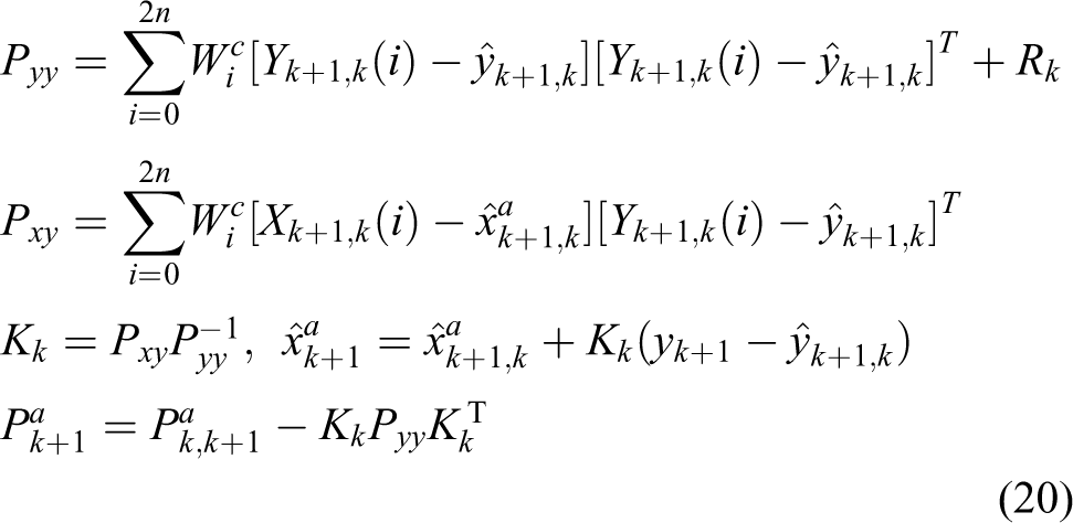
$\begin{array}{l} P_{y y} = \sum_{i = 0}^{2 n} W_{i}^{c} [Y_{k + 1, k} (i) - {\hat{y}}_{k + 1, k}] {[Y_{k + 1, k} (i) - {\hat{y}}_{k + 1, k}]}^{T} + R_{k} \\ P_{x y} = \sum_{i = 0}^{2 n} W_{i}^{c} [X_{k + 1, k} (i) - {\hat{x}}_{k + 1, k}^{a}] {[Y_{k + 1, k} (i) - {\hat{y}}_{k + 1, k}]}^{T} \\ K_{k} = P_{x y} P_{y y}^{- 1}, {\hat{x}}_{k + 1}^{a} = {\hat{x}}_{k + 1, k}^{a} + K_{k} (y_{k + 1} - {\hat{y}}_{k + 1, k}) \\ P_{k + 1}^{a} = P_{k, k + 1}^{a} - K_{k} P_{y y} K_{k}^{T} \end{array}$
20

where R_k is the measurement noise covariance matrix.

Adaptive UKF

In order to further improve the estimation precision, an adaptive adjustment of the noise covariances in the estimation process is implemented using a technique of covariance matching in the UKF context. More specifically, the adaptive estimation of the process noise covariance Q_k and measurement noise R_k on the basis of the pose sequence of the mobile robot will be considered. Therefore, Q_k and R_k are estimated and updated iteratively from the following³⁹

$\begin{array}{l} Q_{k} = K_{k} C_{k} {(K_{k})}^{T} \\ R_{k} = C_{k} + \sum_{i = 0}^{2 n} W_{i}^{c} [Y_{k + 1, k} (i) - {\hat{y}}_{k + 1, k}] {[Y_{k + 1, k} (i) - {\hat{y}}_{k + 1, k}]}^{T} \end{array}$
21

where ${\hat{y}}_{k + 1, k}$ is measured pose of the mobile robot and C_k is defined as

$C_{k} = \sum_{i = k - L + 1}^{k} E_{i} {(E_{i})}^{T}$
22

where $E = {[\begin{matrix} x - \hat{x} & y - \hat{y} & θ - \hat{θ} \end{matrix}]}^{T}$ are the pose estimation errors of the mobile robot at time step k, C_k is an approximation to the covariance of the voltage residual at time step k, and L is window size for covariance matching. More details can be found in the article by Cui et al. (2005)³⁷

Moreover, in order to reduce the chattering of AUKF, a low-pass filter (LPF) is applied to process the estimation signal. A first-order LPF is described in Figure 2.

Figure 2.
Filtering processing of the estimation signal.

The relationship between input u and output y of LPF is given as

$γ \dot{\bar{y}} + \bar{y} = u, \bar{y} (0) = u (0)$
23

where $u = {[{\hat{a}}_{L}, {\hat{a}}_{R}, \hat{δ}]}^{T}$ is estimation output of the AUKF, $γ = diag (γ_{1}, γ_{2}, γ_{3}), γ_{1}, γ_{2}, γ_{3} > 0$ are the filter parameters, $\bar{y}$ is the output, and γ is the filter time constant and a very small value that lies 0≤ γ_i ≤ 1, i = 1, 2, 3.

Remark 3

Note that we employ the first-order LPF (23) to reduce the chattering problem and guarantees smoothness of the estimation signal. After the estimation of the slipping parameters is processed by the LPF, their first-order derivative values ${\dot{\hat{a}}}_{L}$ , ${\dot{\hat{a}}}_{R}$ , and $\dot{\hat{δ}}$ are all bounded.

Design of the tracking controller

Design of the tracking control law

Assume there is a superposition between center of mass and movement geometric center of the WMR. The kinematic model of the WMR with the slipping can be described by equation (8), so actual posture of the WMR is decided by equation (8). The desired posture is defined as p_r = [x_r, y_r, θ_r] ^T , the desired posture satisfies the following equations

$[\begin{matrix} {\dot{x}}_{r} \\ {\dot{y}}_{r} \\ {\dot{θ}}_{r} \end{matrix}] = [\begin{matrix} cos θ_{r} & 0 \\ sin θ_{r} & 0 \\ 0 & 1 \end{matrix}] [\begin{matrix} v_{r} \\ ω_{r} \end{matrix}]$
24

where v_r and ω_r are reference linear velocity and angular velocity of the mobile robot, respectively.

Assumption 4

The reference linear velocity v_r and ω_r as well as their derivatives are all bounded.

Our control objective is to design a trajectory tracking controller, when the wheels’ slipping will occur between the WMR and the ground, which making the actual and desired posture of the WMR satisfy as following

$\lim_{t \to \infty} (p - p_{r}) = 0$
25

In the coordinate frame F₁(x, y), the tracking error dynamics of the WMR are described as follows

$[\begin{matrix} e_{1} \\ e_{2} \\ e_{3} \end{matrix}] = [\begin{matrix} \cos θ + δ sin θ & sin θ - δ \cos θ & 0 \\ - sin θ + δ \cos θ & \cos θ + δ sin θ & 0 \\ 0 & 0 & 1 \end{matrix}] [\begin{matrix} x_{r} - x \\ y_{r} - y \\ θ_{r} - θ \end{matrix}]$
26

where e ₁, e ₂, and e ₃ are state-tracking errors, they are expressed in the frame of real robot, as shown in Figure 3.

Figure 3.
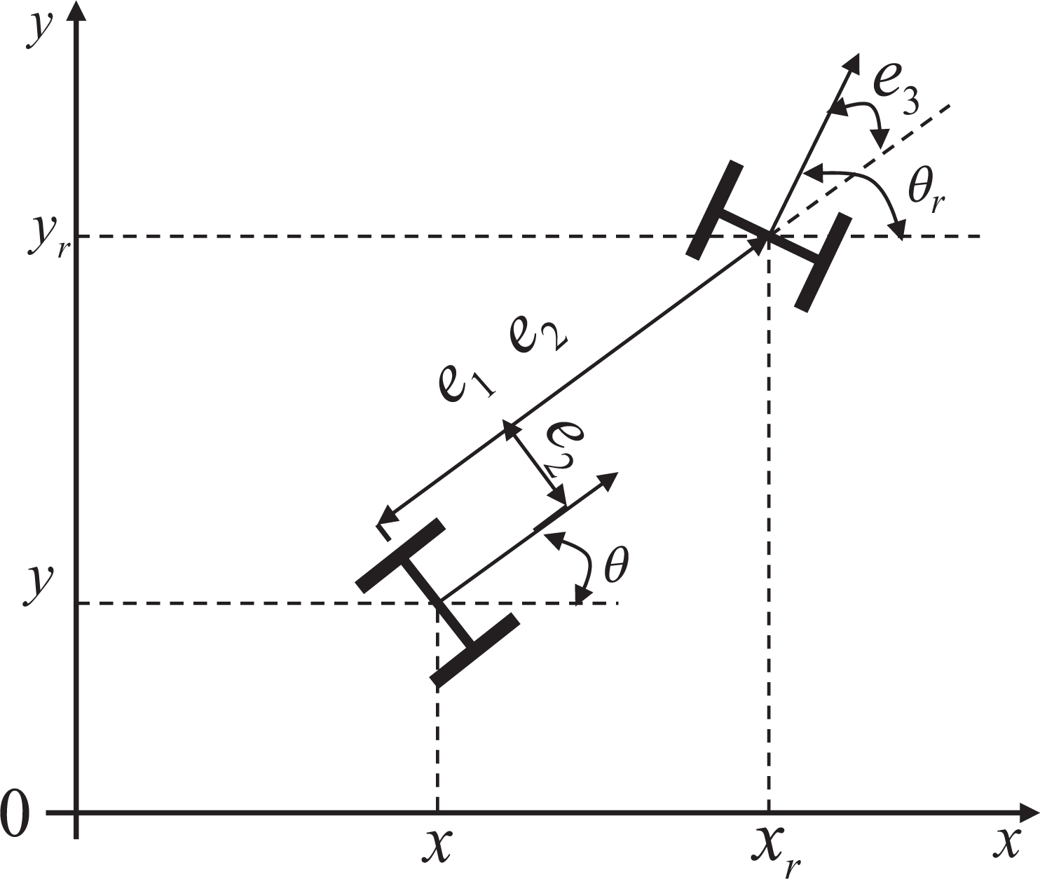
Robotic pose error coordinates scheme.

Tracking errors vector of the WMR is defined as e = [e₁, e₂, e₃] ^T , the error dynamics of the WMR is obtained as follows¹¹

$[\begin{matrix} {\dot{e}}_{1} \\ {\dot{e}}_{2} \\ {\dot{e}}_{3} \end{matrix}] = [\begin{matrix} ω e_{2} + (1 + δ^{2}) v_{r} \cos e_{3} - (1 + δ^{2}) v \\ - ω e_{1} + (1 + δ^{2}) v_{r} sin e_{3} \\ ω_{r} - ω \end{matrix}]$
27

In the presence of the wheels’ slipping, applying backstepping method, the auxiliary control input is designed as follows⁷

$[\begin{matrix} v \\ ω \end{matrix}] = [\begin{matrix} v_{r} \cos e_{3} + k_{1} (v_{r}, ω_{r}) e_{1} \\ ω_{r} + (1 + δ^{2}) k_{2} v_{r} e_{2} + (1 + δ^{2}) k_{3} (v_{r}, ω_{r}) v_{r} sin e_{3} \end{matrix}]$
28

where k ₂ is a positive design constant, and k₁(v_r, ω_r) and k₃(v_r, ω_r) are bounded continuous functions with bounded first derivatives, strictly positive on ℜ × ℜ − (0, 0) .

Now, if the slipping parameters a_R , a_L , and δ that appear in equation (8) are unknown, we cannot choose directly the auxiliary control input as given by equation (28). Hence, we will employ an AuKF with the LPF to attain the estimation of the slipping parameters. If ${\hat{a}}_{R}$ , ${\hat{a}}_{L}$ , and $\hat{δ}$ denote the estimatiotions of a_R , a_L , and δ, respectively, from equations (10) and (28), we can obtain auxiliary control input as follows

$[\begin{matrix} v \\ ω \end{matrix}] = [\begin{matrix} v_{r} \cos e_{3} + k_{1} e_{1} \\ ω_{r} + (1 + {\hat{δ}}^{2}) k_{2} v_{r} e_{2} + (1 + {\hat{δ}}^{2}) k_{3} v_{r} sin e_{3} \end{matrix}]$
29

where k₁ = k₁ (v_r, ω_r) and k₃ = k₃ (v_r, ω_r) are defined in equation (28). Actual control input ω_L and ω_R can also be obtained as follows

$[\begin{matrix} ω_{L} \\ ω_{R} \end{matrix}] = \frac{1}{r} [\begin{matrix} \frac{1}{1 - {\hat{a}}_{L}} & - \frac{b}{2 (1 - {\hat{a}}_{L})} \\ \frac{1}{1 - {\hat{a}}_{R}} & \frac{b}{2 (1 - {\hat{a}}_{R})} \end{matrix}] [\begin{matrix} v \\ ω \end{matrix}]$
30

Remark 4

The estimation values of the slipping parameters are possible to be ones when we use AUKF. Once ${\hat{a}}_{L} = 1$ or ${\hat{a}}_{R} = 1$ , from equation (30), we know that actual control input ω_L or ω_R will go to infinity. This can not be implemented by controller. One way to avoid this is by letting ${\hat{a}}_{L} = 1$ or ${\hat{a}}_{R} = 1$ be replaced by ${\hat{a}}_{L} - \bar{ε}$ or ${\hat{a}}_{R} - \bar{ε}$ ( $\bar{ε}$ is an arbitrarily small positive number).

Control constraints

Because of the bounded velocity capability of the motors, each wheel can achieve a maximum angular velocity ω_max. With the saturation, it is necessary to perform a suitable velocity scaling so as to preserve the curvature radius corresponding to the nominal velocities ω_L and ω_R . The actual commands $ω_{L}^{c}$ and $ω_{L}^{c}$ are then computed by defining

$c = max (\frac{| ω_{L} |}{ω_{max}}, \frac{| ω_{R} |}{ω_{max}}, 1)$
31

From equation (27), the actual commands $ω_{L}^{c}$ and $ω_{R}^{c}$ are computed as follows

$\begin{array}{l} ω_{L}^{c} = ω_{L}, ω_{R}^{c} = ω_{R}, c =1 \\ ω_{L}^{c} = \frac{ω_{L}}{c}, ω_{R}^{c} = ω_{max} sgn (ω_{R}), c = \frac{| ω_{R} |}{ω_{max}} \\ ω_{L}^{c} = ω_{max} sgn (ω_{L}), ω_{R}^{c} = \frac{ω_{R}}{c}, else \end{array}$
32

Remark 5

In equation (32), the nominal velocity control commands ω_L and ω_R are computed from equation (30).

Stability analysis of control system

Theorem 1

The trajectory tracking errors e = [e₁, e₂, e₃] ^T in the tracking error dynamics equation (27) of the WMR with unknown slipping parameters will asymptotically converge to zero vector, if the control law equation (29) and AUKF are applied.

Proof

We choose the following Lyapunov function candidate as

$V (t) = \frac{1}{2} (e_{1}^{2} + e_{2}^{2}) + \frac{1 - \cos e_{3}}{k_{2}}$
33

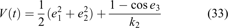
The first-order derivative of the Lyapunov function V(t) can be obtained as

$\dot{V} (t) = e_{1} {\dot{e}}_{1} + e_{2} {\dot{e}}_{2} + \frac{{\dot{e}}_{3} sin e_{3}}{k_{2}}$
34

The error dynamics equation (27) is substituted into equation (34), $\dot{V} (t)$ can be obtain as follows

$\begin{array}{l} \dot{V} (t) = e_{1} [ω e_{2} + (1 + {\hat{δ}}^{2}) v_{r} \cos e_{3} - (1 + {\hat{δ}}^{2}) v] + \\ e_{2} [- ω e_{1} + (1 + {\hat{δ}}^{2}) v_{r} sin e_{3}] + \frac{(ω_{r} - ω) sin e_{3}}{k_{2}} \end{array}$
35

Substituting equation (29) into equation (35), $\dot{V} (t)$ can be obtained as

$\dot{V} (t) = - k_{1} (1 + {\hat{δ}}^{2}) e_{1}^{2} - \frac{k_{3}}{k_{2}} (1 + {\hat{δ}}^{2}) v_{r} {sin}^{2} e_{3}$
36

The domain D is defined by $D = {e \in R^{3} | - π < e_{3} < π}$ , then the Lyapunov function given in equation (33) is positive definite in $D^{'} = {e \in R^{3} | - π < e_{3} < π, e_{3} \neq 0}$ with $\dot{V} (t) \leq 0$ in domain D, so we have

$\dot{V} (t) = - k_{1} e_{1}^{2} (1 + {\hat{δ}}^{2}) - \frac{k_{3}}{k_{2}} (1 + {\hat{δ}}^{2}) v_{r} {sin}^{2} e_{3} \leq 0$
37

As t∈[0,∞), V(t) is a nonincreasing function, we can obtain as

$V (t) \leq V (0), \forall t \geq 0$
38

This implies that V(t) is bounded as t∈[0, ∞). From equaion (33), we know e ₁ and e ₂ are all bounded as t∈[0, ∞). Since desired velocity v_r and ω_r are assumed to be bounded, from equation (28), we know the auxiliary control inputs v and ω are bounded. From equation (27), we can know $\dot{e} = {[{\dot{e}}_{1}, {\dot{e}}_{2}, {\dot{e}}_{3}]}^{T}$ is bounded. The Lyapunov function V(t) is taken the second-order derivative is given as

$\ddot{V} (t) = - {\dot{k}}_{1} e_{1}^{2} (1 + {\hat{δ}}^{2}) - 2 k_{1} (1 + {\hat{δ}}^{2}) e_{1} {\dot{e}}_{1} - 2 k_{1} e_{1}^{2} \hat{δ} \hat{δ} - \frac{{\dot{k}}_{3}}{k_{2}} v_{r} (1 + {\hat{δ}}^{2}) {sin}^{2} e_{3} - \frac{2 k_{3}}{k_{2}} v_{r} \hat{δ} \hat{δ} {sin}^{2} e_{3} - \frac{k_{3}}{k_{2}} {\dot{v}}_{r} (1 + δ^{2}) {sin}^{2} e_{3} - \frac{2 k_{3}}{k_{2}} v_{r} (1 + δ^{2}) {\dot{e}}_{3} sin e_{3} \cos e_{3}$
39

From remark 3, assumption 4, and equation (39), we can know $\ddot{V} (t)$ is bounded, so $\dot{V} (t)$ is uniformly continuous, Barbalat’s Lemma⁴⁰ shows that $\dot{V} (t) \to 0$ as t → ∞. From equation (37), we know e₁ → 0 and e₃ → 0 as t → ∞.

From equations (27) and (29), we have

${\dot{e}}_{3} = - k_{2} v_{r} (1 + {\hat{δ}}^{2}) e_{2} - k_{3} v_{r} (1 + {\hat{δ}}^{2}) sin e_{3}$
40

Thus

$\begin{array}{l} {\ddot{e}}_{3} = - k_{2} {\dot{v}}_{r} (1 + {\hat{δ}}^{2}) e_{2} - 2 k_{2} v_{r} \hat{δ} \hat{δ} e_{2} - k_{2} v_{r} (1 + {\hat{δ}}^{2}) {\dot{e}}_{2} \\ - {\dot{k}}_{3} v_{r} (1 + {\hat{δ}}^{2}) sin e_{3} - k_{3} {\dot{v}}_{r} (1 + {\hat{δ}}^{2}) sin e_{3} \\ - 2 k_{3} v_{r} \hat{δ} \hat{δ} sin e_{3} - k_{3} v_{r} (1 + {\hat{δ}}^{2}) {\dot{e}}_{3} \cos e_{3} \end{array}$
41

Because ${\dot{e}}_{2}$ , ${\dot{e}}_{3}$ , and $\dot{\hat{δ}}$ are all bounded, the reference linear velocity v_r and its derivative are finite value, ${\dot{k}}_{3}$ is bounded, thus ${\ddot{e}}_{3}$ is bounded, that is ${\ddot{e}}_{3} \in L_{\infty}$ , so ${\dot{e}}_{3}$ is uniformly continuous. From Barbalat’s Lemma,⁴⁰ we know ${\dot{e}}_{3} \to 0$ as t → ∞ . Since $e_{3}, {\dot{e}}_{3} \to 0$ as t → ∞, from equation (40), we have $- k_{2} v_{r} (1 + {\hat{δ}}^{2}) e_{2} \to 0$ as t → ∞. If the reference linear velocity v_r ≠ 0 as t → ∞, then e₂ → 0 as t → ∞.

In conclusion, the equilibrium point e = [e₁, e₂, e₃] ^T = [0, 0, 0]^T is uniform and asymptotically stable. This implies the WMR can converge asymptotically to the reference posture p_r = [x_r, y_r, θ_r] ^T from the arbitrary initial posture. Thus, the control objective is implemented accordingly.

Adaptive adjustment of control parameters

Since the location of the poles determines the damping ratio ξ of transient response near the reference trajectory, so the transient response of closed-loop robot system can be analyzed from the location of the poles in a closed-loop system. The theory of the location of poles shows that the poles are always in the area not exceeding ±45^∘ in the left-half s-plane. That is to say, $\cos 45^{\circ} \leq ξ \leq 1$ is guaranteed. It implies the transient response of trajectory tracking always converges without oscillation regardless of gain parameters. Therefore, we need not choose carefully the gain parameters to reduce oscillation or overshoot.

The tracking error vector of the WMR is defined as e = [e₁, e₂, e₃]^T, after substituting equation (28) into equation (27), the tracking error differential equations of closed-loop robotic system can be obtained as

$[\begin{matrix} {\dot{e}}_{1} \\ {\dot{e}}_{2} \\ {\dot{e}}_{3} \end{matrix}] = [\begin{matrix} - k_{1} (1 + {\hat{δ}}^{2}) e_{1} + [ω_{r} + k_{2} (1 + {\hat{δ}}^{2}) v_{r} e_{2} + k_{3} (1 + {\hat{δ}}^{2}) sin e_{3}] e_{2} \\ - [ω_{r} + k_{2} (1 + {\hat{δ}}^{2}) v_{r} e_{2} + k_{3} (1 + {\hat{δ}}^{2}) sin e_{3}] e_{1} + v_{r} (1 + {\hat{δ}}^{2}) sin e_{3} \\ - k_{2} (1 + {\hat{δ}}^{2}) v_{r} e_{2} - k_{3} (1 + {\hat{δ}}^{2}) sin e_{3} \end{matrix}]$
42

After linearizing the equation (42) around the equilibrium point [e₁, e₂, e₃] ^T = [0, 0, 0] ^T , we have

$\begin{array}{l} [\begin{matrix} {\dot{e}}_{1} \\ {\dot{e}}_{2} \\ {\dot{e}}_{3} \end{matrix}] = [\begin{matrix} - k_{1} (1 + {\hat{δ}}^{2}) & ω_{r} & 0 \\ - ω_{r} & 0 & (1 + {\hat{δ}}^{2}) v_{r} \\ 0 & - k_{2} (1 + {\hat{δ}}^{2}) v_{r} & - k_{3} (1 + {\hat{δ}}^{2}) \end{matrix}] [\begin{matrix} e_{1} \\ e_{2} \\ e_{3} \end{matrix}] \\ = A_{q} e \end{array}$
43

Remark 6

Note that the mismatch between the linearized model and the nonlinear system grows for values of e ₃ far from zero. It will be shown that, in practice, after the transient, e ₃ remains very close to zero. Then, the problem could be present at the first instants, due to the initial condition. For that reason, we assume that, in practice, the real robot and the reference virtual robot start close. In this case, the linearization is successful.

Generally, the trial-and-error method is used to determine controller gains. If so, not only the accuracy of the controlled robotic system can not be guaranteed but also its adaptation is bad. Based on the linearization model, an online computing method of control gains is proposed by the pole placement strategy.

The controller gains can be determined by comparing the actual and desired characteristic polynomial equations. Here, pole placement methodology is employed to decide control gains of robotic tracking controller. The desired poles are chosen as $s_{1} = - 2 ξ ω_{n}$ and $s_{2}, s_{3} = - ξ ω_{n} \pm j ω_{n} \sqrt{1 - ξ^{2}}$ (ξ is damping ratio of controlled mobile robot system and ω_n is the characteristic frequency of controlled WMR). So the desired characteristic polynomial of the closed-loop robotic system takes the following form as:

$(s + 2 ξ ω_{n}) (s^{2} + 2 ξ ω_{n} s + ω_{n}^{2})$
44

where ξ is desired damping coefficient of closed-loop robotic system, ω_n is the characteristic frequency, both of them are positive constants, and s is Laplace operator.

Equation (43), the characteristic polynomial of the system matrix A_q can be obtained as

$\det (s I - A_{q}) = s^{3} + (k_{1} + k_{3}) (1 + {\hat{δ}}^{2}) s^{2} + [k_{1} k_{3} {(1 + {\hat{δ}}^{2})}^{2} + k {(1 + {\hat{δ}}^{2})}^{2} v_{r}^{2} + ω_{r}^{2}] s + k_{1} k_{2} {(1 + {\hat{δ}}^{2})}^{3} v_{r}^{2} + k_{3} ω_{r}^{2} (1 + {\hat{δ}}^{2})$
45

The robotic closed-loop poles are now equal to the roots of the characteristic polynomial equation (45). Comparing equation (44) with equation (45), the following equations can be obtained as

$(k_{1} + k_{3}) (1 + {\hat{δ}}^{2}) = 4 ξ ω_{n} k_{1} k_{3} {(1 + {\hat{δ}}^{2})}^{2} + k_{2} {(1 + {\hat{δ}}^{2})}^{2} v_{r}^{2} + ω_{r}^{2} = 4 ξ^{2} ω_{n}^{2} + ω_{n}^{2} k_{1} k_{2} {(1 + {\hat{δ}}^{2})}^{3} v_{r}^{2} + k_{3} ω_{r}^{2} (1 + {\hat{δ}}^{2}) = 2 ξ ω_{n}^{3}$
46

Equation (46), we can obtained as

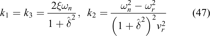
$k_{1} = k_{3} = \frac{2 ξ ω_{n}}{1 + {\hat{δ}}^{2}}, k_{2} = \frac{ω_{n}^{2} - ω_{r}^{2}}{{(1 + {\hat{δ}}^{2})}^{2} v_{r}^{2}}$
47

where ω_n should be larger than the maximum-allowed robotic angular velocity, ω_n > ω_rmax, ω_rmax is the maximum-allowed robot angular velocity. ω_rmax can be obtained as follows

$ω_{r max} = \frac{4 r ω_{max}}{b}$
48

where ω_max is robot’s wheel, which can achieve the maximum angular velocity, r is radius of the wheels, and b is the distance between two driving wheels. In equation (47), v_r → 0 and k₂ → ∞. One way to avoid this is by allowing the closed-loop poles only depend on the values of v_r and ω_r . Consequently, a gain scheduling should be chosen for $ω_{n} = \sqrt{ω_{r}^{2} + d {(1 + {\hat{δ}}^{2})}^{2} v_{r}^{2}}$ with a positive constant d. Then, the control gains can become

$k_{1} = k_{3} = \frac{2 ξ \sqrt{ω_{r}^{2} + d {(1 + {\hat{δ}}^{2})}^{2} v_{r}^{2}}}{1 + {\hat{δ}}^{2}}, k_{2} = d$
49

Remark 7

In equation (49), the slipping parameter δ is estimated by AUKF online (see “Scheme of the robotic slipping parameter estimation” section).

Remark 8

From assumption 1 and equation (49), we know that k_i ∈ (0, ∞),(i=1, 2, 3) are realizable in physics.

Since the dynamic performance of closed-loop system is determined by the damping ratio ξ, thus we can predetermine the damping ratio ξ in accordance with the desired performance requirements. Therefore, controller gains k ₁, k ₂, and k ₃ can be determined only by adjusting parameter d, and then the control parameter adjusting process is simplified greatly. Since the reference velocity v_r and ω_r are time varying, then the control gains k ₁ and k ₃ are also time varying. Accordingly, they can be adjusted online in accordance with equation (49). Hence, the real-time property and flexibility of the controlled robot system are improved greatly.

From the above analysis (see “A scheme of the robotic slipping parameter estimation,” “Design of the tracking controller,” and “Adaptive adjustment of control parameters” sections), tracking close-loop control principle of the WMR can be described by the scheme shown in Figure 4.

Figure 4.
A scheme of the trajectory tracking control principle for the WMR. WMR: wheeled mobile robot.

Simulations and experiment

Simulations

In this section, to verify the effectiveness of the proposed tracking control scheme, some simulations are performed on the kinematic model of the tracked WMR with slipping. In the simulations, the angular velocities of the two driving wheels are considered as control input variables. To observe and compare the simulation results more easily, two kinds of reference trajectories are chosen as follows: one is a straight-line trajectory, and the other is a circle one. The parameters of the WMR are chosen as follows:

b = 1 m, r = 0.125 m, ξ = 0.707 (both to ensure that convergence speed of the tracking errors and ensure that as far as possible little overshoot, the best damping ratio ξ = 0.707 is chosen), robot's wheels can achieve a maximum angular velocity ω_max = 8.5rad/s, k ₂ = d = 60; the parameters of the AUKF should be determined carefully. For the AUKF, the three constant filter parameters are chosen as follows: α = 1, β = 2 and γ = 0, L = 100. The parameters of the LPF are chosen as follows: γ₁ = 0.6, γ₂ = 0.2, γ₃ = 0.8. Let us suppose the three states about the robot's poses, which can be measured directly.

Note that the kinematics and the dynamics of the robot are described by the continuous-time equations and (26). On the other hand, the AUKF is a discrete-time algorithm. Thus, to perform the computer simulation, the continuous-time equations (8) and (26) are discretized using Euler’s forward difference scheme with a sampling period of T_s = 0.02 s.

The straight-line reference trajectory tracking

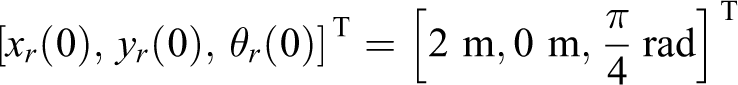
In this case, a straight-line reference trajectory is considered. The initial posture of the reference trajectory is set at

${[x_{r} (0), y_{r} (0), θ_{r} (0)]}^{T} = {[0 m,0 m, \frac{π}{4} rad]}^{T}$

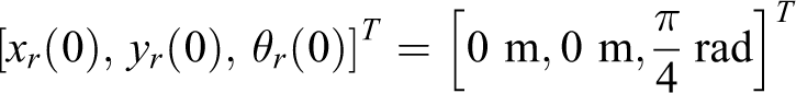
The actual initial posture of the WMR is given as

${[x (0), y (0), θ (0)]}^{T} = {[- 2 m, - 2 m, \frac{π}{4} rad]}^{T}$

The actual initial posture errors of the WMR is

${[e_{1} (0), e_{2} (0), e_{3} (0)]}^{T} = {[2 \sqrt{2} m,0 m, 0 rad]}^{T}$

Reference velocities are given as v_r = 2 m/s, ω_r = 0 rad/s, and the reference orientation angle θ_r = π rad/4. In order to demonstrate the tracking performance, abrupt changes are simulated to occur in the three slipping parameters at time t = 15 s, they are given as follows:

$\begin{array}{l} a_{L} = {\begin{cases} 0.15 sin 0.2 (t - 15), t \geq 15 s \\ 0, else \end{cases} \\ a_{R} = {\begin{cases} - 0.15 sin 0.2 (t - 15), t \geq 15 s \\ 0, else \end{cases} \\ δ = {\begin{cases} 0.12 sin 0.2 (t - 15), t \geq 15 s \\ 0, else \end{cases} \end{array}$

From Figure 5, we can see that proposed control method can track the desired straight-line trajectory rather quickly. Furthermore, when the wheel’s slipping are introduced into the robot’s system, we can observe that the proposed adaptive tracking controller has excellent ability to overcome the wheel’s slipping perturbation. Meanwhile, we can see that the AUKF can estimate the time-varying slipping parameters rather precisely. The estimations of the slipping parameters have a rather light oscillation due to LPF is applied.

Figure 5.
Straight-line trajectory tracking. (a) Straight-line trajectory tracking result; (b) x orientation error e ₁; (c) y orientation error e ₂; (d) heading angle error e ₃; (e) slipping parameter a_L estimation; (f) slipping parameter a_R estimation; (g) slipping parameter δ estimation; (h) control input ω_L ; (i) control input ω_R ; (j) control gains (k₁ = k₃).

The circle reference trajectory tracking

The equation of the circle reference trajectory is given as

${\begin{cases} x_{r} = 2 \cos t \\ y_{r} = 2 sin t \end{cases}$

where t is simulation time. The initial posture of the reference trajectory is set at

${[x_{r} (0), y_{r} (0), θ_{r} (0)]}^{T} = {[2 m,0 m, \frac{π}{4} rad]}^{T}$

The actual initial posture of the WMR is

${[x (0), y (0), θ (0)]}^{T} = {[- 1 m,0 m, \frac{π}{4} rad]}^{T}$

The actual initial posture errors of the WMR is

${[e_{1} (0), e_{2} (0), e_{3} (0)]}^{T} = {[3 m,0 m, 0 rad]}^{T}$

To facilitate comparison of the simulation results, the control parameters, the parameters of the AUKF, and the changes of the slipping parameters are all the same as in the previous simulation. In this case, the reference line velocity v_r(t) = 2 rad/s, and the tangential angle velocity of each point on the reference trajectory is given as follow: ω_r(t) = 1 rad/s.

From Figure 6, we can see that the proposed control approach has the good tracking control performance for the curved path in spite of the effects of the unknown wheels’ slipping. That is to say, the proposed control method can effectively conquer the slipping effect for the given curved trajectory tracking of the WMR. Meanwhile, the AUKF can estimate three time-varying slipping parameters accurately, even when sudden changes happen.

Figure 6.
Circle trajectory tracking. (a) Circle trajectory tracking result; (b) x orientation error e ₁ ; (c) y orientation error e ₂; (d) heading angle error e ₃; (e) slipping parameter a_L estimation; (f) slipping parameter a_R estimation; (g) slipping parameter δ estimation; (h) control input ω_L ; (i) control input ω_R ; (j) control gains (k₁ = k₃).

Furthermore, from Figures 5 and 6, we can futher find that the proposed control method can effectively overcome the slipping for the given trajectory tracking of the WMR, this is mainly because that the designed tracking controller have an adaptive ability, whose some control parameters k ₁ and k ₃ can be adaptively modifying in real time. Moreover, even if the wheels’ slipping parameters change suddenly, the AUKF can still exactly estimate slipping parameters in real time to satisfy the demands of the robot in the actual working environment. Consequently, the adaptive tracking control algorithm has good robustness and adaptive ability to confront slipping parameter perturbations of the WMR.

Further, by comparing Figure 5 with Figure 6, we can also find that the tracking errors of circle trajectory is bigger than straight-line trajectory, this is mainly because that circle path have a time-varying reference angular velocity θ_r while reference angular velocity of the straight-line reference path is constant. Compared Figure 5(j) with Figure 6(j), we can see that k ₁ and k ₃ are all constants in straight-line trajectory environment, from equation (47), we know $k_{1} = k_{3} = 2 ξ v_{r} \sqrt{d} = 21.9056$ . However, in circular reference trajectory environment, due to reference angular velocity θ_r is time-varying, control gains k ₁ and k ₃ must also be time varying to meet better circular reference trajectory.

Real experiment

In order to demonstrate the effectiveness and applicability of the proposed method, a real-time control system is implemented for the mobile robot. In the experiment, a mobile robot with one vision navigation system fixed on the top moves along the marking line. Figure 7 shows the picture of the robot which is used in the experiment. It has the same structure as Figure 8, with two driving wheels and two passive wheels. The diameter of the robot is 50 cm and the radius of driving wheel is 12.5 cm. The driving wheels are driven by motors with the maximum permissible speed of 3900 n/min. The motor and the driving wheel are connected by a reduction gearbox. For the convenience of comparing, the control parameters are all same as the simulations.

Figure 7.
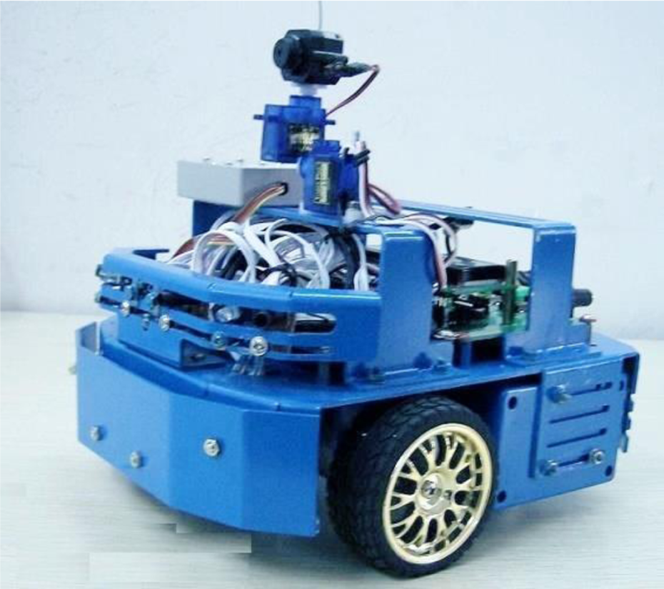
Mobile robot in real experiment.

Figure 8.
Schematic diagram of the experiment control system.

The control board of the mobile robot consists of the main controller and motor controller. The main controller of the robot is dsPIC30F6014, which is running at 32 MHz. It is used to communicate with host computer and motor controller. It receives the voltage instruction from the host computer and calculates the voltage distribution on the right and left motors, respectively, and then sends the data through SPI communication to the auxiliary motor controller, dsPIC4012. The motor controller generates pulse-width modulation (PWM) signal with different duty cycles according to the voltage instruction.

Figure 8 shows the whole schematic diagram of the trajectory tracking system for the mobile robot. Because of the complexity of the calculation process, the proposed adaptive tracking controller based on AUKF is carried out in the main computer running at the frequency of 1.86 MHz. The software for implementing the algorithm is developed in Visual C++6.0. After the reference trajectory has been set up, the proposed adaptive tracking controller generates the real voltage instruction. The dsPIC controller can generate the PWM signal to control the velocity of the mobile robot so that the mobile robot moves according to the instruction. The vision navigation system evaluates the posture of the robot and feedback the information to the host computer until the posture error is minimized.

In order to validate the applicability of the proposed control scheme, the mobile robot was required to track reference trajectories. The real position of the mobile robot is feedback to the mobile robot every 0.2 s by camera navigation system.

In order to prove the effectiveness of the proposed adaptive tracking controller based on AUKF, real experiment is implemented for the desired trajectory of a straight line. Reference velocities are given as v_r = 2 m/s and ω_r = 0 rad/s, The robot started tracking with initial errors e₁ = 0 m, e₂ = 0 m, and e₃ = 0 rad. At 25 s, the arbitrary external wheels’ slipping disturbance is fed in robotic system by laying sand on the ground. The experimental results are shown in Figure 9. From Figure 9, we can see that the tracking errors of the proposed adaptive control algorithm are asymptotically convergent. It implies that the mobile robot eventually approaches the reference trajectory with asymptotic stability within 3 s to 0.32% error bound by the proposed adaptive controller. This fact demonstrates the effectiveness of the proposed adaptive control algorithm.

Figure 9.
Experimental results for the straight-line tracking errors with initial error (0 m, 0 m, 0 rad).

Conclusions

The wheels’ slipping effects appear generally in practice and are really significant problems for the control of the WMR. In this article, the wheels’ slipping is taken into account and modeled as three time-varying parameters. The kinematic model containing the slipping parameters is proposed and AUKF is designed to estimate unknown slipping. The estimated results are introduced into a uniformly asymptotically stable tracking controller to implement the path tracking objective. Furthermore, based on pole placement strategy, the controller parameters are adjusted online in real time in accordance with the practial reference trajectory. The simulation and real experiment results are given to validate the performance of the proposed tracking control approach. More works should be done to research the physical mechanism of slipping and the dynamic tracking controller design will be investigated in future.

Footnotes

Acknowledgement

Authors Mingyue Cui, Hongzhao Liu, Wei Liu and Rongjie Huang are also affiliated with Oil Equipment Intelligent Control Engineering Laboratory of Henan province, Nanyang, Henan, 473061, China.

Declaration of conflicting interests

The author(s) declared no potential conflicts of interest with respect to the research, authorship, and/or publication of this article.

Funding

The author(s) disclosed receipt of the following financial support for the research, authorship, and/or publication of this article: This work was supported by the National Natural Science Foundation (no.U1404614), the Henan Province Education Department Foundation (no.14B120003 and no.17A413002), and the Henan Province Scientific and Technological Foundation (no. 142300410455).

References

Yang

Kim

. Sliding mode control of trajectory tracking of nonholonomic wheeled mobile robots. IEEE Trans Robot Autom 1999; 15( 3 ): 578–587.

Chwa

. Sliding-mode control of nonholonomic wheeled mobile robots in polar coordinates. IEEE Trans Contr Syst Technol 2004; 12( 4 ): 637–644.

Park

Yoo

Park

. Adaptive neural sliding mode control of nonholonomic wheeled mobile robots with model uncertainty. IEEE Trans Contr Syst Technol 2009; 17( 1 ): 207–214.

Chen

Yeh

. EP-based kinematic control and adaptive fuzzy sliding-mode dynamic control for wheeled mobile robots. Inf Sci 2009; 179(1): 180–195.

Zhang

Chung

JH,

Velinsky

. Variable structure control of a differentially steered wheeled mobile robot. J Intell Robot Syst 2003; 36(3): 301–314.

Yang

Zheng

. Extended state observer based double loop integral sliding mode control of electronic throttle valve. IEEE Trans Intell Transp Syst 2015; 16(5): 2501–2510.

Fukao

Nakagawa

Adachi

. Adaptive tracking control of a nonholonomic mobile robot. IEEE Trans Robot Autom 2000; 16( 5 ): 609–615.

Dixon

Queiroz

Dawson

. Adaptive tracking and regulation of a wheeled mobile robot with controller/update law modularity. IEEE Trans Contr Syst Technol 2004; 12( 1 ): 138–147.

Dong

Kuhnert

. Robust adaptive control of nonholonomic mobile robot with parameter and nonparameter uncertainties. IEEE Trans Robot 2005; 21( 2 ): 261–266.

10.

Jiang

Pan

. Simultaneous tracking and stabilization of mobile robots: an adaptive approach. IEEE Trans Autom Cont 2004; 49( 7 ): 1147–1152.

11.

Ranjbarsahraei

Roopaei

Khosravi

. Adaptive fuzzy formation control for a swarm of non-holonomic differentially driven vehicles. Nonlinear Dynam 2012; 67(4): 2747–2757.

12.

Jiang

Nijmeijer

. Tracking control of mobile robots: a case study in backstepping. Automatica 1997; 33( 7 ): 1393–1399.

13.

Dong

Huo

Tso

. Tracking control of uncertain dynamic nonholonomic system and its application to wheeled mobile robots. IEEE Trans Robot Autom 2000; 16( 6 ): 870–874.

14.

Lee

Song

Lee

. Tracking control of unicycle-modeled mobile robots using a saturation feedback controller. IEEE Trans Contr Syst Technol 2001; 9( 2 ): 305–318.

15.

Sousa

Hemerly

Galvao

. Adaptive control for mobile robot using wavelet networks. IEEE Trans Syst Man Cybern B 2002; 32( 4 ): 493–504.

16.

Fierro

Lewis

. Control of a nonholonomic mobile robot using neural networks. IEEE Trans Neural Netw 1998; 9( 4 ): 589–600.

17.

Yoo

Choi

Park

. Generalized predictive control based on self-recurrent wavelet neural network for stable path tracking of mobile robots: adaptive learning rates approach. IEEE Trans Circuits Syst I: Reg Papers 2006; 53( 6 ): 1381–1394.

18.

Hendzel

. An adaptive critic neural network for motion control of a wheeled mobile robot. Nonlinear Dynam 2007; 50(4): 849–855.

19.

Yen

THS

Chang

. Design of a robust neural network-based tracking controller for a class of electrically driven nonholonomic mech- anical systems. Inform Sci 2013; 222(3): 559–575.

20.

Das

Kar

. Design and implementation of an adaptive fuzzy logic-based controller for wheeled mobile robots. IEEE Trans Contr Syst Technol 2006; 14( 3 ): 501–510.

21.

Hwang

Chang

. Network-based fuzzy decentralized sliding-mode control for car-like mobile robots. IEEE Trans Ind Electron 2007; 54( 1 ): 574–585.

22.

Martínez

Castillo

Aguilar

. Optimization of interval type-2 fuzzy logic controllers for a perturbed autonomous wheeled mobile robot using genetic algorithms. Inform Sci 2009; 179(13): 2158–2174.

23.

Castillo

Martínez-Marroquín

Melin

. Comparative study of bio-inspired algorithms applied to the optimization of type-1 and type-2 fuzzy controllers for an autonomous mobile robot. Inform Sci 2012; 192(6): 19–38.

24.

Klančar

Matko

Blažič

. A control strategy for platoons of differential drive wheeled mobile robot. Robot Autonom Syst 2011; 59(2): 57–64.

25.

Zheng

. Evaluating the performance of vehicular platoon control under different network topologies of initial states. Phys A 2016; 450: 359–368.

26.

Cui

Huang

Liu

. Adaptive tracking control of wheeled mobile robots with unknown longitudinal and lateral slipping parameters. Nonlinear Dynam 2014; 78(3): 1811–1826.

27.

Tian

Sarkar

. Control of a mobile robot subject to wheel slip. J Intell Robot Syst 2014; 74(3-4): 915–929.

28.

Yoo

. Adaptive tracking and obstacle avoidance for a class mobile robots in the presence of unknown skidding and slipping. IET Contr Theory Appl 2011; 5(14): 1597–1608.

29.

Cui

Sun

Liu

. Adaptive tracking and obstacle avoidance control for mobile robots with unknown sliding. Int J Adv Robot Syst 2012; 9( 171 ): 1–14.

30.

Wang

Low

. Modeling and analysis of skidding and slipping in wheeled mobile robots: control design perspective. IEEE Trans Robot 2008; 24( 3 ): 676–687.

31.

Low

Wang

. GPS-based path following control for a car-like wheeled mobile robot with skidding and slipping. IEEE Trans Contr Syst Technol 2008; 16( 2 ): 340–347.

32.

Low

Wang

. GPS-based tracking control for a car-like wheeled mobile robot with skidding and slipping. IEEE Trans Mechat 2008; 13(4): 480–484.

33.

Gonzalez

Fiacchini

Alamo

. Adaptive control for a mobile robot under slip conditions using an LMI-based approach. Eur J Contr 2010; 16(2): 144–155.

34.

Iossaqui

Camino

Zampieri

. A nonlinear control design for tracked robots with longitudinal slip. In: Preprints of the 18th IFAC World Congress, Milano, Italy, 28 August–2 September, 2011, 44(1): 5932–5937. ELSEVIER.

35.

Zhou

Han

Dai

. Backstepping based global exponential stabilization of a tracked mobile robot with slipping perturbation. J Bionic Eng 2011; 8(1): 69–76.

36.

Brunke

Campbell

. Estimation architecture for future autonomous vehicles. In: IEEE the Proceedings of the American Control Conference, Anchorage, AK, 8–10 May 2002, pp. 1108–1114. IEEE.

37.

Cui

Hong

Layne

. A comparison of nonlinear filtering approaches with an application to ground target tracking. Signal Proc 2005; 85(8): 1469–1492.

38.

Julier

Uhlmann

JH,

Durrant-Whyte

. A new method for the nonlinear transformation of means and covariances in filters and estimators. IEEE Trans Autom Contr 2000; 45(3): 477–482.

39.

Song

Han

. An adaptive UKF algorithm for the state and parameter estimations of a mobile robot. Acta Autom Sin 2008; 34(1): 72–79.

40.

Slotine

. Applied nonlinear control. New Jersey: Prentice-Hall, 1991.

An adaptive unscented Kalman filter-based adaptive tracking control for wheeled mobile robots with control constrains in the presence of wheel slipping

Abstract

Keywords

Introduction

Kinematic model of the WMR with wheels’ slipping

Assumption 1

Remark 1

Assumption 2

Remark 2

Assumption 3

A scheme of the robotic slipping parameter estimation

Standard UKF

Adaptive UKF

Remark 3

Design of the tracking controller

Design of the tracking control law

Assumption 4

Remark 4

Control constraints

Remark 5

Stability analysis of control system

Theorem 1

Proof

Adaptive adjustment of control parameters

Remark 6

Remark 7

Remark 8

Simulations and experiment

Simulations

The straight-line reference trajectory tracking

The circle reference trajectory tracking

Real experiment

Conclusions

Footnotes

Acknowledgement

Declaration of conflicting interests

Funding

References