Sage Journals: Discover world-class research

Abstract

We investigate the dynamic mode of a 3-degree of freedom (DOF) redundantly actuated parallel manipulator by taking the flexible deformation of the limbs into account. The dynamic model is derived using Newton–Euler formulation. Since the number of equations derived from the force and moment equilibrium of the parallel manipulator components is less than the number of unknown variables, the flexible deformation of the limbs is treated as an inequality constraint to find the solution of the dynamic model. The errors of moving platform caused by the flexible deformation of limbs are discussed, and a control strategy is given. To validate the model, the dynamic model is integrated with the control system and compared with the traditional method to minimize the normal driving forces.

Keywords

Parallel manipulator force optimization actuation redundancy dynamics deformation

Introduction

Over the last decade, parallel robots have received great attention in both theoretical research and practical applications. This attention is due to their superior stiffness, high load to weight ratio, and low inertia over the conventional serial manipulators that are made with rigid-body links and joints connected in serial. Parallel manipulators have wide application in the industrial world;^1,2 for example, flight simulators,³ parallel kinematics machines,⁴ and conveyors for the pretreatment and electrocoating of a vehicle body.⁵ However, parallel manipulators have two inherent disadvantages: (i) limited workspace due to the mobility constraints imposed by the other legs in the mechanism and (ii) singular configurations that further reduce the useful workspace. To deal with these drawbacks, several proposals have been presented, among which actuation redundancy is an effective solution. Redundantly actuated parallel manipulators have attracted a lot of interest.^6

–10

To provide high accuracy while performing fast motions, the dynamics modeling must be efficiently formulated in order to meet real-time requirements. There are four main methods to model the dynamic equations:¹¹ Newton–Euler formulation,¹² Lagrangian formulation,¹³ virtual work principle,¹⁴ and Kane’s method.¹⁵ As opposed to non-redundant parallel manipulators, the dynamics of redundantly actuated parallel manipulators are statically undetermined and have infinite possible solutions. An optimization technique to minimize an objective function while satisfying the dynamic equations should be used to obtain a unique solution to the inverse dynamics. Many studies have been conducted on the dynamics of redundantly actuated parallel manipulators. Nahon and Angeles¹⁶ used a quadratic-programming approach by minimizing the internal forces in the system to obtain real-time solutions to the force optimization problem of redundantly actuated parallel manipulators. Cheng et al.¹⁷ used the Moore–Penrose pseudoinverse to find the solution of a 2-DOF redundant parallel manipulator. However, flexible deformation of the manipulator is generally neglected in dynamic models. In fact, deformation of the mechanisms has an important effect on the accuracy of a redundant parallel manipulator, in particular for heavy loads and high-speed motions. Some researchers attempted to derive the dynamics of redundant parallel manipulators by introducing the deformation compatibility equation. Liu et al.¹⁸ and Xu et al.¹⁹ introduced the deformation compatibility equation to deal with the dynamics of the redundant parallel manipulator. The work on the dynamics of redundant parallel manipulators that considers flexible deformation is scarce, and the bending deformation of the limb of the parallel manipulator is not considered.

We investigate the dynamic model of a novel 3-DOF redundantly actuated parallel manipulator. The dynamic model is derived using the Newton–Euler formulation, and both the axial and bending deformations of the limbs are taken as an inequality constraint to find the solution of the dynamic model. Based on the dynamic model presented, a driving forces optimization is introduced, which can improve the motion accuracy of the tool tip, and the dynamic model is incorporated into a control system. This article is organized as follows. The section “Kinematics” gives the structure description and kinematics, which are used to derive the force and moment equilibrium equation of the manipulator components in the section “Dynamic model of the parallel manipulator.” The section “Driving force optimization” investigates the flexible deformation of limbs to provide the inequality constraint to the dynamic model. The section “Control application” deals with the control application of the dynamic model. Conclusions are presented in the section “Conclusions.”

Kinematics

Structure description and inverse kinematics

A schematic diagram of the 3-DOF redundant parallel manipulator is shown in Figure 1 and the corresponding kinematic model is given in Figure 2. It is composed of a moving platform linked to the base by two RPU (R, P, and U standing for rotational, prismatic and universal joints, respectively) limbs, one RPS (S standing for spherical joint), and one UPU limb. All the prismatic joints in the four limbs are active. The limbs are numbered 1–4. The first, third, and fourth limbs are coplanar and the two rotational axes of the U joint connecting the moving platform of one limb are parallel to the two rotational axes of the U joint connecting the moving platform of other limb, respectively.

Figure 1.

Three-dimensional model of the parallel manipulator.

Figure 2.

Kinematic model of the parallel manipulator.

The base coordinate O − XYZ is fixed on point B₄ with a vertical Z axis. The Y axis is along the vector from B₄ to B₁, and the X axis satisfies the right-hand rule. Meanwhile, a moving coordinate system $O' - X' Y' Z'$ is attached to point A₄ with the Z′ axis normal to the moving platform and the Y′ axis along the vector from A₄ to A₁. The moving platform can translate along the Z axis and rotate about the X axis and Y axis while it is actuated by the four prismatic inputs. Thus, the parallel manipulator is redundantly actuated.

The geometrical parameters are defined as $O' A_{i} = R_{1} (i = 1, 2, 3), O B_{i} = R_{2} (i = 1, 2, 3), and A_{i} B_{i} = L_{i} (i = 1, 2, 3, 4)$ . The Euler angle is used to describe the orientation of the manipulator. The rotational matrix from $O' - X' Y' Z'$ to O − XYZ can be expressed as

R = [\begin{matrix} \cos α_{2} & 0 & sin α_{2} \\ sin α_{1} sin α_{2} & \cos α_{1} & - sin α_{1} \cos α_{2} \\ - \cos α_{1} sin α_{2} & sin α_{1} & \cos α_{1} \cos α_{2} \end{matrix}]

where α₁ and α₂ are the rotation angles of platform around the X and Y axes, respectively.

The translational DOF along the Y axis is restricted by the second limb, but the unwanted parasitic motion along the Y axis exists because of the S joint of the second limb when the orientation of the moving platform changes.

Let ${r'}_{a i}$ be the position vector of joint point A_i in the moving coordinate system $O' - X' Y' Z'$ . The position vector of joint point A_i in the base coordinate system O − XYZ can be expressed as

r_{a i} = R {r'}_{a i} + r_{a 4} (i = 1, 2, 3, 4)

where $r_{a 4}$ is the position vector of point O′ in O − XYZ and $r_{a 4} = {[0 y_{P} z]}^{T}$ , of which the Z component is z and y_p is the parasitic motion.

For point A₂, $r_{a 2} = {[R_{1} \cos α_{2} R_{1} sin α_{1} sin α_{2} + y_{P} z - R_{1} \cos α_{1} sin α_{2}]}^{T}$ . Since the R joint in the second limb can only rotate around the Y axis and the Y component of $r_{a 2}$ should be zero. Thus, we can get

R_{1} sin α_{1} sin α_{2} + y_{P} = 0

Thus, the parasitic motion in the Y direction can be determined based on equation (3). The constraint equation associated with each limb can be written as

L_{i} = ‖ r_{a i} - r_{b i} ‖

where r _bi is the position vector of joint point B_i in O − XYZ. So the input vector of the parallel manipulator can be expressed as $V_{input} = {[L_{1} L_{2} L_{3} L_{4}]}^{T}$ , while the output vector of the moving platform is $V_{output} = {[α_{1} α_{2} z]}^{T}$ .

The vector loop equation for each kinematic chain in O − XYZ can be written as

r_{a i} = r_{b i} + L_{i} n_{i}

where n _i is the unit vector of link A_iB_i and the direction of n _i is from point B_i to point A_i.

The position vector of mass center C_i of the lower part of link A_iB_i in O − XYZ can be expressed as

r_{c i} = r_{b i} + \frac{L_{c}}{2} n_{i}

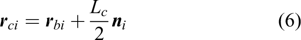
where L_c is the length of lower part of link A_iB_i. The position vector of mass center D_i of the upper part of limb A_iB_i can be written as

r_{d i} = r_{b i} + (L_{i} - \frac{L_{d}}{2}) n_{i}

where L_d is the length of upper part of link A_iB_i. Because the moving platform is an isosceles right triangle, the position vector of the mass center of the moving platform can be expressed as

r_{C} = \frac{1}{3} r_{a 2} + \frac{2}{3} r_{a 4}

Velocity analysis

Choosing point B_i as the center of rotation of link A_iB_i and taking the derivative of equation (5) with respect to time leads to

{\dot{r}}_{a i} = {\dot{L}}_{i} n_{i} + L_{i} (ω_{i} \times n_{i})

where ω _i is the angular velocity of link A_iB_i, and taking the dot product with n _i on both sides of equation (9) leads to

{\dot{L}}_{i} = n_{i}^{T} {\dot{r}}_{a i}

Taking the cross product with n _i on both sides of equation (9) leads to equation (11)

ω_{i} = \frac{1}{L_{i}} (n_{i} \times {\dot{r}}_{a i})

Differentiating equation (6) with respect to time leads to

{\dot{r}}_{ci} = \frac{L_{c}}{2} ω_{i} \times n_{i}

Taking the derivative of equation (7) with respect to time leads to

{\dot{r}}_{di} = (L_{i} - \frac{L_{d}}{2}) ω_{i} \times n_{i} + {\dot{L}}_{i} n_{i}

Dynamic model of the parallel manipulator

Acceleration analysis

Differentiating equation (9) with respect to time yields equation (14)

r_{a i} = {\ddot{L}}_{i} n_{i} + 2 {\dot{L}}_{i} (ω_{i} \times n_{i}) + L_{i} ω_{i} \times (ω_{i} \times n_{i}) + L_{i} ɛ_{i} \times n_{i}

where ε _i is the angular acceleration of link A_iB_i.Taking the dot product with n _i on both sides of equation (14) leads to

{\ddot{L}}_{i} = n_{i}^{T} r_{a i} + L_{i} ω_{i}^{2}

The angular acceleration ε _i can be obtained by taking the cross product with n _i on both sides of equation (14) leading to

ɛ_{i} = \frac{1}{L_{i}} (n_{i} \times r_{a i} - 2 {\dot{L}}_{i} ω_{i})

Differentiating equation (12) with respect to time yields

r_{c i} = \frac{L_{c}}{2} (ɛ_{i} \times n_{i} - ω_{i}^{2} n_{i})

The acceleration of the mass center of the upper part of link A_iB_i can be obtained by differentiating equation (13) to give

r_{d i} = (L_{i} - \frac{L_{d}}{2}) (ɛ_{i} \times n_{i} - ω_{i}^{2} n_{i}) + 2 ω_{i} \times {\dot{L}}_{i} n_{i} + {\ddot{L}}_{i} n_{i}

Dynamic model

For a less-DOF parallel machine, its limbs contribute not only to transmitting driving forces/torques but also to providing constraint forces/torques. If all the constraint forces/torques are taken into account, there will be too many redundant forces/torques that will make the dynamic model much more complicated. To simplify the problem, it is assumed that only the force in Z axis and the moments around the X and Y axes are imposed on the moving platform. The free-body diagram of link A_iB_i is shown in Figure 3.

Figure 3.

Free-body diagram of link A_iB_i.

The Euler equation of link A_iB_i with respect to O − XYZ is given by

\frac{L_{c} m_{c}}{2} n_{i} \times (g - r_{c i}) + (L_{i} - \frac{L_{d}}{2}) m_{d} n_{i} \times (g - r_{d i}) + L_{i} n_{i} \times F_{A i} - J_{i} ɛ_{i} + M_{B i} = 0

Where $F_{A i} = F_{A i l} + F_{A i v}$ are the forces imposed by the platform on the link; F _Bi is the constraint force that the base imposes on link A_iB_i; M _Bi is the constraint moment imposed on point B_i; $- m_{c} {\ddot{r}}_{c i} and - m_{d} {\ddot{r}}_{d i}$ are inertial forces of the lower and upper parts of link A_iB_i, respectively; g is the acceleration vector of gravity; and J_i is the moment of inertia of link A_iB_i about point B_i.

Taking the cross product with n _i on both sides of equation (19) leads to

F_{A i}_{v} = \frac{1}{L_{i}} (n_{i} \times \frac{L_{c}}{2} m_{c} n_{i} \times (g - r_{c i}) + n_{i} \times (L_{i} - \frac{L_{d}}{2}) m_{d} n_{i} \times (g - r_{d i}) - n_{i} \times J_{i} ɛ_{i} + n_{i} \times M_{B i})

Based on the orientation of R joints in the first, second, and third limbs, we conclude that M _B1 and M _B3 only have a Y directional component and M _B2 only has a X directional component. For the fourth limb, there is a U joint connecting to the base instead of an R joint, so we can get $M_{B 4} = 0$ .

Based on Figure 4, the Newtonian equation of the moving platform can be written as

M g + F_{ext} - M r_{C} - \sum_{i = 1}^{4} (F_{A i l} + F_{A i v}) = 0

Figure 4.

Free-body diagram of moving platform.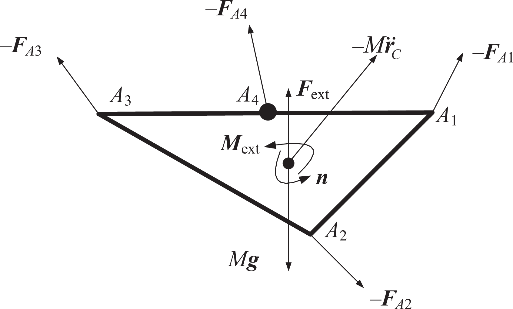

where M is the mass of the moving platform and F _ext is the external force acting on the moving platform. The Euler equation of the moving platform is given by

- J_{x} ɛ_{x} - J_{y} ɛ_{y} - J_{z} ɛ_{z} - \sum_{i = 1}^{3} {r'}_{i} \times (F_{A i l} + F_{A i v}) + M_{ext} + {r'}_{C} \times (M g - M r_{C} + F_{ext}) = 0

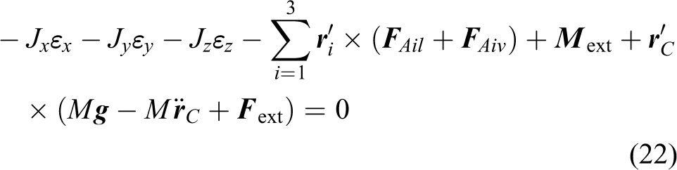
where J_x, J_y, and J_z are moments of inertia of X′, Y′, and Z′ axes about point A₄, respectively, and ε _x , ε _y , and ε _z represent, respectively, the angular accelerations about the X′, Y′, and Z′ axes. $r_{i}^{'} (i = 1, 2, 3)$ is the vector from point A₄ to point $A_{i} (i = 1, 2, 3), {r'}_{C}$ is the vector from point A₄ to point C, and M _ext is the external moment acting on the moving platform.

Combining equations (21) and (22) with equation (20) leads to

Q a = b

where $a = {(F_{A 1 l}, F_{A 2 l}, F_{A 3 l}, F_{A 4 l}, M_{B 1}, M_{B 2}, M_{B 3})}^{T}$ . There are six static force equations and seven unknown variables in equation (23). Thus, the optimization technique should be used to obtain the inverse solution of the dynamics.

Driving force optimization

Deformations of non-redundant links

In practical applications, the limb with lowest stiffness in the manipulator has a flexible deformation. If this deformation is not considered, the motion accuracy of the manipulation is low. Here, the flexible deformation of the limb is considered. Based on the structure of the redundant parallel manipulator in this article, the deformations of the joints, base, and moving platform can be ignored. Because the non-redundant limbs (the first, second, and third limbs) are driven with a position control model and the redundant limb (the fourth limb) is driven with a force control model, which will be discussed in detail in the section “Control application,” we mainly investigate the deformations of the non-redundant limbs. There are two kinds of deformations of link A_iB_i. As shown in Figure 5, the axial deformation leads to the axial error δL_il and the bending deformation leads to the tangential error δL_iv.

Figure 5.

Deformation diagrams of link A_iB_i.

The force of link A_iB_i has to be analyzed to obtain the deformation of the limb.¹⁸ The force analysis of link A_iB_i is shown in Figure 6, where m(u) g represents the distributed gravity on the link, $- m (u) {\ddot{r}}_{i} (u)$ is the distributed inertial force on the link, and ${\ddot{r}}_{i} (u)$ is the acceleration of the point with the distance of u to point B_i. ${\ddot{r}}_{i} (u)$ can be obtained using the acceleration analysis method in the subsection “Acceleration analysis,” and ${\ddot{r}}_{i} (u)$ can be expressed as

r_{i} (u) = {\begin{matrix} ɛ_{i} \times (u n_{i}) - ω_{i}^{2} (u n_{i}) \\ ɛ_{i} \times L_{c} n_{i} - ω_{i}^{2} L_{c} n_{i} + {\ddot{L}}_{i} n_{i} + 2 ω_{i} \times {\dot{L}}_{i} n_{i} + ɛ_{i} \times (u - L_{c}) n_{i} - ω_{i}^{2} (u - L_{c}) n_{i} \end{matrix} \begin{matrix} (0 \leq u \leq L_{c}) \\ (L_{c} \leq u \leq L_{i}) \end{matrix}

Figure 6.

Force analysis diagram of link A_iB_i.

First, let us focus on the axial deformation. Since the prismatic joint of each limb is actuated by a servomotor via a ball screw, both the upper and lower parts of each limb have axial deformations. Because the overlap of the upper and lower parts of limb is relatively short, while its stiffness is large, the axial deformation of overlap is neglected. For link $A_{i} B_{i} (i = 1, 2, 3)$ , taking point B_i as the original point, the force of the point with the distance of u to point B_i can be expressed as

F_{d i} (u) = {\begin{matrix} n_{i}^{T} \cdot \int_{u}^{L_{c}} \frac{m_{c} (g - r_{i} (u))}{L_{c}} d u + n_{i}^{T} \cdot \int_{L_{i} - L_{c}}^{L_{i}} \frac{m_{d} (g - r_{i} (u))}{L_{d}} d u + F_{A i l} (0 \leq u \leq L_{i} - L_{d}) \\ n_{i}^{T} \cdot \int_{u}^{L_{i}} \frac{m_{d} (g - r_{i} (u))}{L_{d}} d u + F_{A i l} (L_{c} \leq u \leq L_{i}) \end{matrix}

The axial deformation of link A_iB_i can be expressed as

δ L_{i l} = \int_{0}^{L_{i} - L_{d}} \frac{F_{d i} (u)}{E S_{B}} d u + \int_{L_{c}}^{L_{i}} \frac{F_{d i} (u)}{E S_{A}} d u

where S_A and S_B are the cross-sectional areas of the upper and lower part of link A_iB_i, respectively, and E is the elastic modulus.

The first, third, and fourth limbs are coplanar (O − YZ plane), and the second limb is located in the vertical plane (O − XZ plane). As mentioned in the section “Dynamic model of the parallel manipulator,” the constraint moment M _B2 is in the direction of the Y axis according to the orientation of the R joint of the second limb, so the bending deformation of the second limb occurs along the Y axis when the constraint force F _A2v is applied on A₂. In addition, the U joint of the second limb connecting to the moving platform cannot limit the motion along the Y axis of the limb. Thus, the bending deformation of the second limb along the Y axis is similar to that of a cantilever.

Similarly, based on the abovementioned analysis, motions of the end point A₁ and A₃ of the first and third limbs along the X axis are limited due to the R joints, so the bending deformation of the first and third limb is along the X axis. Unlike the second limb, the first and third limbs are coplanar (O − YZ plane), so the stiffness of these limbs along the X axis is relatively large and the influence on the error of the end point is small so the bending deformations of the first and third limbs can be neglected. Thus, only the bending deformation of the second limb is taken into consideration here.

Because the gravity and inertia moment of the link are smaller than constraint force, thus only the constraint force F _A2v is taken into account. According to equation (20), we get

F_{A 2}_{v} = \frac{1}{L_{2}} (n_{2} \times \frac{L_{c}}{2} m_{c} n_{2} \times (g - r_{c 2}) + n_{2} \times (L_{2} - \frac{L_{d}}{2}) m_{d} n_{2} \times (g - r_{d 2}) - n_{2} \times J_{2} ɛ_{2} + n_{2} \times M_{B 2})

As mentioned earlier, the bending deformation of the second limb can be seen as that of a cantilever, and the bending stiffness of the lower limb and the overlap of the upper and lower limbs is relatively large so that their bending deformation can be neglected. According to the knowledge of mechanics of materials,²⁰ the displacement of the end of a cantilever can be obtained by solving the differential equation for small deflection of cantilever of linear elastic material, it can be expressed as

δ L = \frac{P}{E I} \frac{L^{3}}{3}

where P is the force acting on the end point of the cantilever, L is the length of the cantilever, and I is the moment of inertia of the cantilever cross section about the neutral axis. For upper part of link A_iB_i, I can be expressed as $π d^{4} / 64$ , where d is the diameter of the upper part of limb A_iB_i. So by letting $P = e_{2}^{T} F_{A 2}_{v}$ , where $e_{2} = {[0 1 0]}^{T}$ is the unit vector along Y axis, and $L = L_{2} - L_{c}$ , the bending deformation of the second limb along the Y axis can be expressed as

δ L_{2 v} = \frac{e_{2}^{T} F_{A 2}_{v} {(L_{2} - L_{c})}^{3}}{3 E I}

Platform displacement caused by the link deformation

The position vector of point A₄ (origin of moving coordinate system $O' - X' Y' Z'$ ) in the base coordinate system O − XYZ can be expressed as

r_{a 4} = r_{b i} + L_{i} n_{i} - R \cdot {r'}_{a i} (i = 1, 2, 3)

The deformations of link A_iB_i lead to the errors of the moving platform including the rotation error $δ α_{1}, δ α_{2}$ , and the translation error δz. As a result, the rotational matrix R is turned into R + δR and equation (1) can be rewritten as

R + δ R = [\begin{matrix} \cos (α_{2} + δ α_{2}) & 0 & sin (α_{2} + δ α_{2}) \\ sin (α_{1} + δ α_{1}) sin (α_{2} + δ α_{2}) & \cos (α_{1} + δ α_{1}) & - \cos (α_{2} + δ α_{2}) sin (α_{1} + δ α_{1}) \\ - \cos (α_{1} + δ α_{1}) sin (α_{2} + δ α_{2}) & sin (α_{1} + δ α_{1}) & \cos (α_{1} + δ α_{1}) \cos (α_{2} + δ α_{2}) \end{matrix}]

For limbs 1 and 3, r _a4, L_i, and n _i in equation (30) are changed into $r_{a 4} + δ r_{a 4}, L_{i} + δ L_{i l}, and n_{i} + δ n_{i}$ , and equation (30) should be rewritten as

r_{a 4} + δ r_{a 4} = r_{b i} + (L_{i} + δ L_{i l}) (n_{i} + δ n_{i}) - (R + δ R) \cdot {r'}_{a i}_{} (i = 1, 3)

According to the analysis in the section “Kinematics,” we can get $r_{a 4} = {[0, y_{P}, z]}^{T} = {[0, - R_{1} sin α_{1} sin α_{2}, z]}^{T}$ . Considering the errors caused by the deformation, r _a4 can be rewritten as

r_{a 4} + δ r_{a 4} = {[0, - R_{1} sin (α_{1} + δ α_{1}) sin (α_{2} + δ α_{2}) + δ L_{2 v}, z + δ z]}^{T}

By eliminating equation (30) from equation (32) and then neglecting high-order small quantities, we can obtain

L_{i} δ n_{i} + n_{i} δ L_{i l} - δ R \cdot {r'}_{a i} = δ r_{a 4}

Considering n _i is an unit vector and δ_ni is perpendicular to n _i , taking the dot product of equation (34) with n _i at both sides yields

δ L_{i l} = n_{i}^{T} (δ r_{a 4} + δ R \cdot {r'}_{a i})

Based on the analysis in the subsection “Deformations of non-redundant links,” the bending deformation of the second limb should be taken into account. For the second limb, equation (30) can be rewritten as

r_{b 2} + (L_{2} + δ L_{2 l}) (n_{2} + δ n_{2}) + δ L_{2 v} e_{2} - (R + δ R) \cdot {r'}_{a 2} = r_{a 4} + δ r_{a 4}

By eliminating equation (30) from equation (36) and then taking dot product of equation (36) with n ₂ on both sides yields

δ L_{2 l} + δ L_{2 v} e_{2}^{T} n_{2} = n_{2}^{T} (δ r_{a 4} + δ R \cdot {r'}_{a 2})

Based on equations (35) and (37), we can obtain the relationship between the deformations of non-redundant limbs and the kinematic errors of moving platform as

W {(δ α_{1}, δ α_{2}, δ z)}^{T} = {(δ L_{1 l} - n_{1 y} δ L_{2 v}, δ L_{2 l}, δ L_{3 l} - n_{3 y} δ L_{2 v})}^{T}

where $W = [\begin{matrix} R_{1} (- n_{1 y} (\cos α_{1} sin α_{2} + sin α_{1}) + n_{1 z} \cos α_{1}) & - R_{1} n_{1 y} sin α_{1} \cos α_{2} & n_{1 z} \\ R_{1} n_{2 z} sin α_{1} sin α_{2} & R_{1} (- n_{2 x} sin α_{2} - n_{2 z} \cos α_{1} \cos α_{2}) & n_{2 z} \\ R_{1} (n_{3 y} (sin α_{1} - \cos α_{1} sin α_{2}) - n_{3 z} \cos α_{1}) & - R_{1} n_{3 y} sin α_{1} \cos α_{2} & n_{3 z} \end{matrix}], n_{i} = {[n_{i x} n_{i y} n_{i z}]}^{T}, (i = 1, 2, 3)$ .

Objective function

In practical applications, a tool is fixed on the moving platform, and the parallel manipulator can be used to develop the tool. Let the tool length be L_t and the tool be fixed at point A₄. The tool length vector is along the Z′ axis. Based on the dynamic model presented earlier, we can improve the position accuracy of the tool tip by optimizing the driving forces of the manipulator. Thus, the optimizing object is to lower the error of the tool tip, which is caused by both axial and bending deformations of the limbs, to a minimum. The objective function can be expressed as

H = \min (δ x_{t}^{2} + δ y_{t}^{2} + δ z_{t}^{2})

where δ_xt, δ_yt, and δ_zt are the errors of the tool tip in the X, Y, and Z axes, respectively. Combining equation (23) and (38) leads to

ℜ \cdot p = q

where $p = {(F_{A 1 l}, F_{A 2 l}, F_{A 3 l}, F_{A 4 l}, M_{B 1}, M_{B 2}, M_{B 3}, δ α_{1}, δ α_{2}, δ z)}^{T}$ . There are 10 unknown variables and 9 equations in equation (40). The general solution of equation (40) can be expressed as

p = λ p_{0} + p_{s}

where p _s is a special solution of equation (41), p ₀ is a base value, and λ is a real number. So the position vector of the tool tip point T of the machine tool can be expressed as

t = r_{a 4} + R \cdot t'

where $t = {(x_{t}, y_{t}, z_{t})}^{T}$ is the position vector of point T in the base coordinate system, and $t' = {(0, 0, L_{t})}^{T}$ is the position vector of point T in the moving coordinate system $O' - X' Y' Z'$ . Considering the kinematic errors of the moving platform, equation (42) can be rewritten as

t + δ t = (r_{a 4} + δ r_{a 4}) + (R + δ R) \cdot t'

where $δ t = {(δ x_{t}, δ y_{t}, δ z_{t})}^{T}$ . Based on equations (42) and (43), we can get

δ t = δ r_{a 4} + δ R \cdot t'

Equation (44) can be written in the matrix format as

{(δ x_{t}, δ y_{t}, δ z_{t})}^{T} = D {(δ α_{1}, δ α_{2}, δ z)}^{T} + δ L_{2 v} e_{2}

where $D = [\begin{matrix} 0 & L_{t} \cos α_{2} & 0 \\ - R_{1} \cos α_{1} sin α_{2} - L_{t} \cos α_{1} \cos α_{2} & - R_{1} sin α_{1} \cos α_{2} + L_{t} sin α_{1} sin α_{2} & 0 \\ - L_{t} sin α_{1} \cos α_{2} & - L_{t} \cos α_{1} sin α_{2} & 1 \end{matrix}]$ .

Equation (45) shows the relationship between link deformation and the errors of the tool tip. Since the optimization goal is to minimize the error of the tool tip, $δ d_{s} = {(δ α_{1 s}, δ α_{2 s}, δ z_{s})}^{T} and δ d_{0} = {(δ α_{10}, δ α_{20}, δ z_{0})}^{T}$ are derived from the 8th, 9th, and 10th elements of vector p from equation (41). Thus, we can get

δ t = λ \cdot D δ d_{0} + D δ d_{s} + δ L_{2 v} e_{2}

To minimize δt², the following equation should be satisfied

\frac{\partial δ t^{2}}{\partial λ} = 2 ((D δ d_{s} + δ L_{2 v} e_{2})^{T} + λ D δ d_{0}^{T}) D δ d_{0} = 0

Based on equation (47), λ can be determined by

λ = \frac{- (D δ d_{s} + δ L_{2 v} e_{2})^{T} D δ d_{0}}{D δ d_{0}^{T} D δ d_{0}}

Substituting equation (48) into equation (41), the drive forces can be determined.

Control application

Control scheme

The control strategy of a redundant parallel manipulator is more complicated than that of non-redundant one, and for the redundantly actuated manipulator, position and force control are widely used.^21,22 For the 3-DOF redundantly actuated parallel manipulator in this article, the redundant limb is controlled with a force control mode and the non-redundant limbs are controlled with a position control mode. As for position control mode, it consists of a current loop, a velocity loop, and a position loop. The expected input positions of the non-redundant limbs (L₁, L₂, and L₃) come from the inverse kinematics equation (3) in the subsection “Structure description and inverse kinematics.” For force control mode, sections “Dynamic model of the parallel manipulator” and “Driving force optimization” build the dynamic model of the parallel manipulator and optimize the driving force, finally by substituting equation (48) into equation (41) in the subsection “Objective function,” we can get the optimized driving forces as the expected driving force of the redundant limb. The control scheme of the redundant parallel manipulator is shown in Figure 7.

Figure 7.

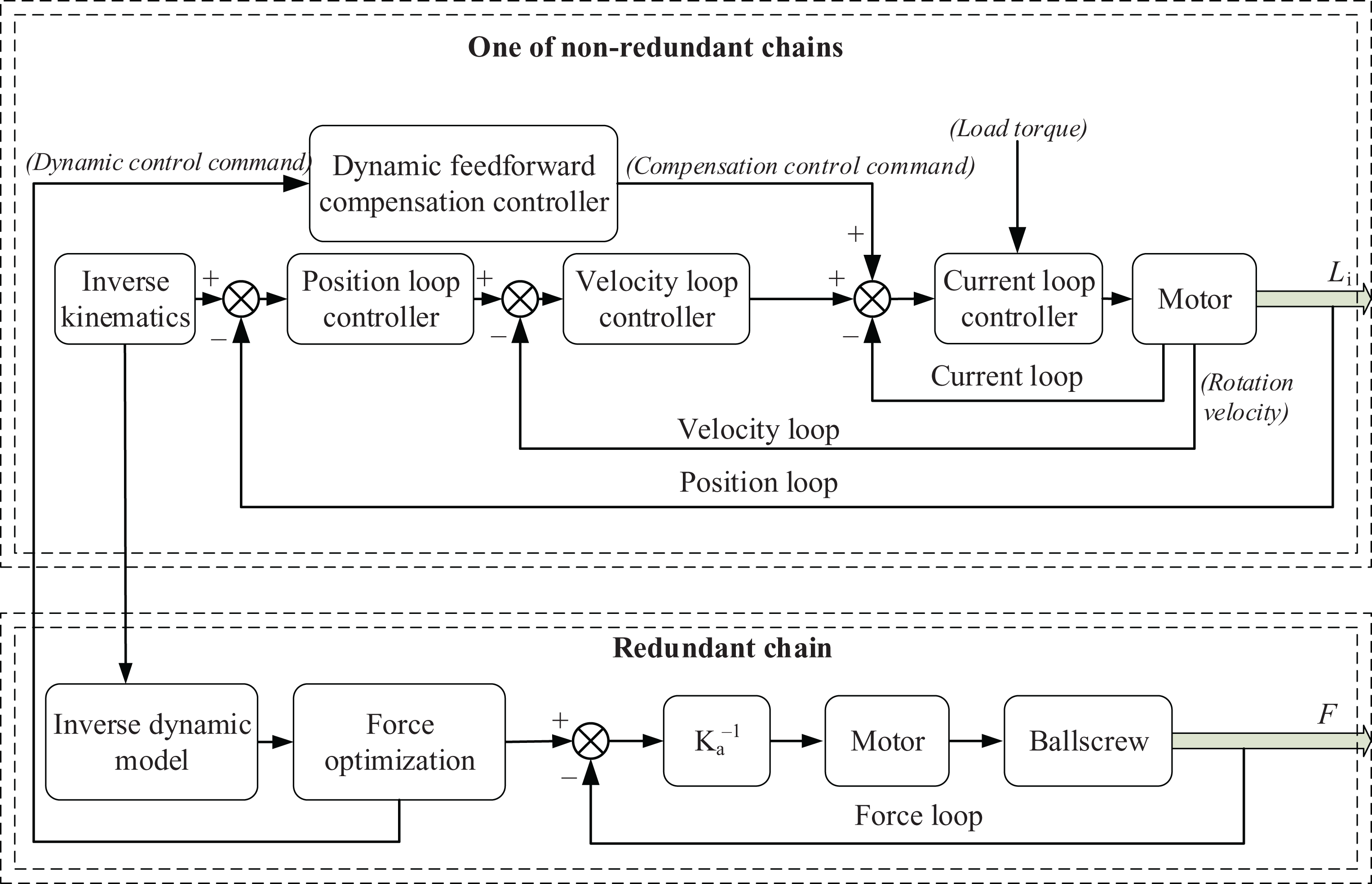
Schematic diagram of control system.

Besides, for the non-redundant limbs, the load torque as a kind of nonlinear effect on the servomotor will affect the accuracy of the output of the servomotor. As the dynamic model is built and the driving force optimization is applied, the load force of each actuator link during the machine running can be obtained from equation (48). As mentioned earlier, each limb of the redundantly actuated parallel manipulator is actuated by a servomotor via a ball screw and the pitch of lead screw is known, so the load torque of each servomotor can be calculated. Thus, the nonlinear effect on the servomotor caused by the load torque can be compensated by a dynamic feedforward compensator. As shown in Figure 7, the transfer function from the input of compensation control command to the output of rotation velocity is G₁(s), and the transfer function from the input of load torque to the output of rotation velocity is G₂(s), in order to improve the output accuracy of the servomotor by compensating the nonlinear effect caused by the load torque, the transfer function of the dynamic feedforward compensation controller G_df(s) should satisfy the following equation

G_{d f} (s) G_{1} (s) + G_{2} (s) = 0

It should be noted that more future research about the control system is required to improve the performance of the controller in real-world application. For example, intelligence control such as neural control and fuzzy control might be needed to solve the problem of disturbance of this manipulator.^23,24 But before that, the efforts on the dynamic model and optimization are also very necessary and meaningful for improving the accuracy of the tool tip.

Results

The geometrical and inertial parameters of the manipulator are given in Table 1. The dynamics and control are simulated when the tool moves along the trajectory shown in Figure 8. In the motion, the acceleration of translational motion of the moving platform is given by

a = {\begin{cases} - \frac{a_{0}}{T_{t}} t + a_{0} (0 < t \leq T_{t}) \\ 0 (T_{t} < t \leq T_{f} - T_{t}) \\ - \frac{a_{0}}{T_{t}} (t - T_{f} + T_{t}) (T_{f} - T_{t} < t \leq T_{f}) \end{cases}

Table 1.

The geometrical and inertial parameters of the manipulator.

Parameters	Values	Parameters	Values
M	80 kg	L_t	0.15 m
R ₁	0.4 m	L_c	0.6 m
R ₂	0.6 m	L_d	1.0 m
J_x	2.133 kg·m²	S_A	1.30 × 10⁻³ m²
J_y	2.133 kg·m²	S_B	0.55 × 10⁻³ m²
J_z	4.267 kg·m²	m_c	9.8646 kg
I	1.2566 × 10⁻⁷ m²	m_d	2.6043 kg
E	210 GPa

Figure 8.

Simulation trajectory.

where T_t is the acceleration/deceleration time, T_f is the total run time, and a₀ is the maximum acceleration.

Similarly, the angular acceleration of the moving platform is given by

ε = {\begin{cases} - \frac{ε_{0}}{T_{t}} t + ε_{0} (0 < t \leq T_{t}) \\ 0 (T_{t} < t \leq T_{f} - T_{t}) \\ - \frac{ε_{0}}{T_{t}} (t - T_{f} + T_{t}) (T_{f} - T_{t} < t \leq T_{f}) \end{cases}

where ε₀ is the maximum angular acceleration. In the simulation, $T_{f} = 1 s, T_{t} = 0.4286 s, a_{0} = 0.3267 {m/s}^{2} =, and ε_{0} = 3.4208 {rad/s}^{2}$ . The output vector V _output cited in the section “Kinematics” changes from [0° 0° 1.15 m] to [30° 30° 1.2 m], and the coordinate of tool tip T in O − XYZ changes from [0, 0, 1.3]^T to [0.075, −0.165, 1.3125]^T. In addition, a 1000 N external force is imposed on point A₄ vertically downward.

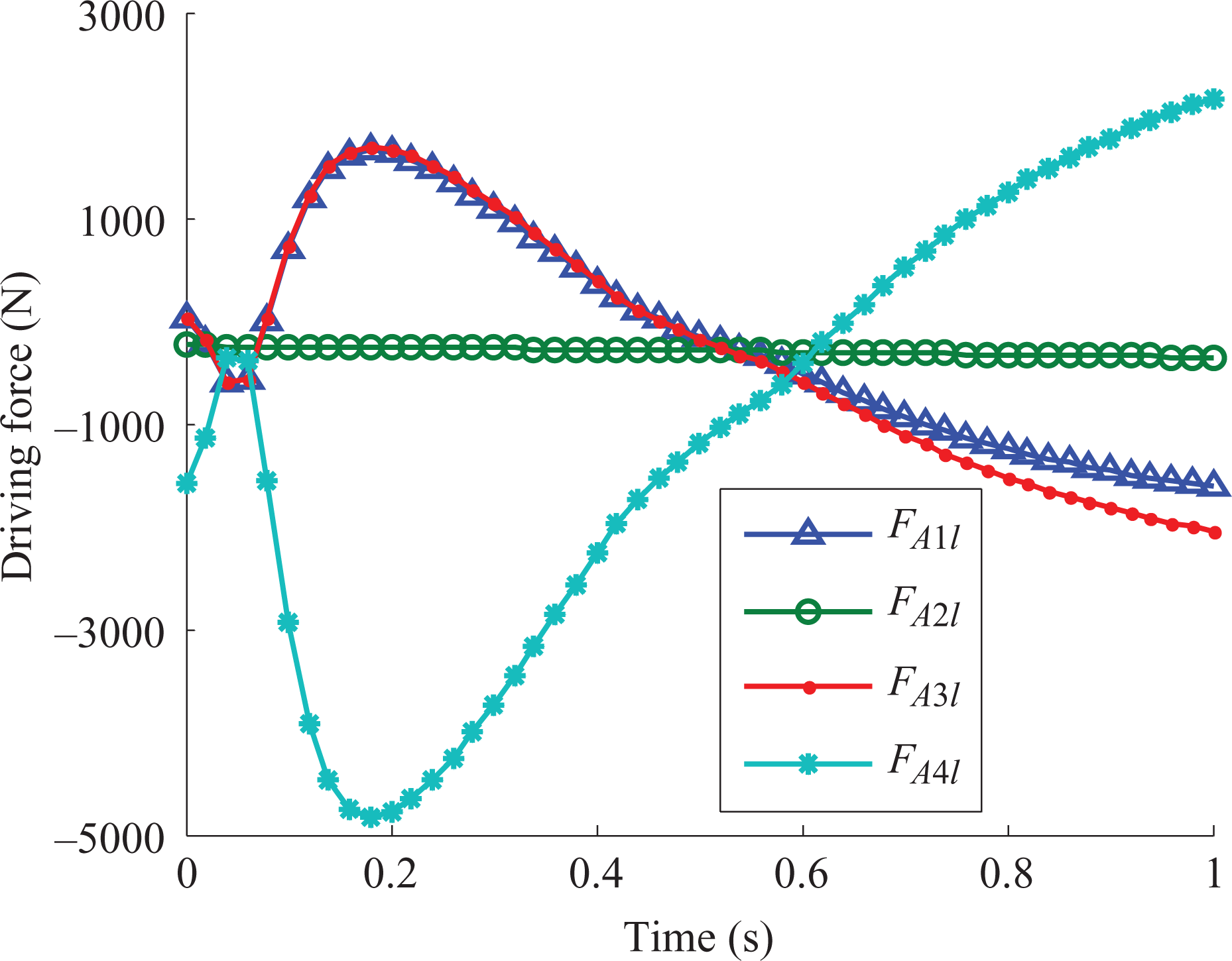
As the driving forces directly affect the deformations of the limbs, they can also be minimized to improve the position error. Thus, the traditional driving force optimization method, which aims to minimize the driving forces (optimization goal: $H = \min \sum_{i = 1}^{4} {(F_{i l})}^{2}$ ), is introduced for comparison.^25,26 For ease of description, the driving force optimization method proposed in this article is called method I, and the traditional driving force optimization method is called method II. The driving forces of the parallel manipulator obtained using method I and method II are shown in Figures 9 and 10, respectively.

Figure 9.

Driving forces in method I.

Figure 10.

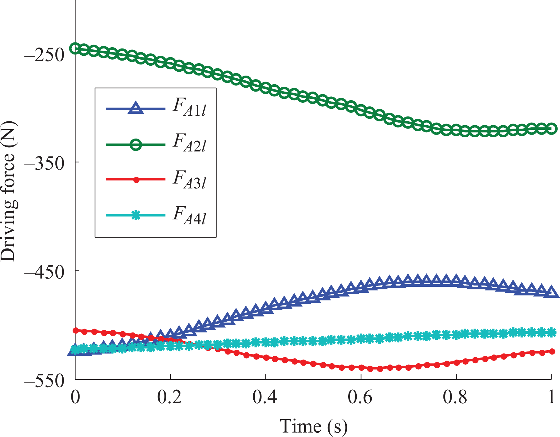
Driving forces in method II.

In the rigid-body dynamic model, the flexible deformation of limb is neglected, and the position of the tool tip can be obtained based on the rigid-body model. If the flexible deformation of limbs is considered, the position of tool tip will be different from the values in the rigid-body model. Here, the difference between the tool tip position computed from the model that considers the limb deformation and the tool tip position computed from the rigid-body model is defined as the position error. When methods I and II are used, the position errors are simulated as shown in Figure 11 and we can see that the position error can be greatly reduced when method I is used. 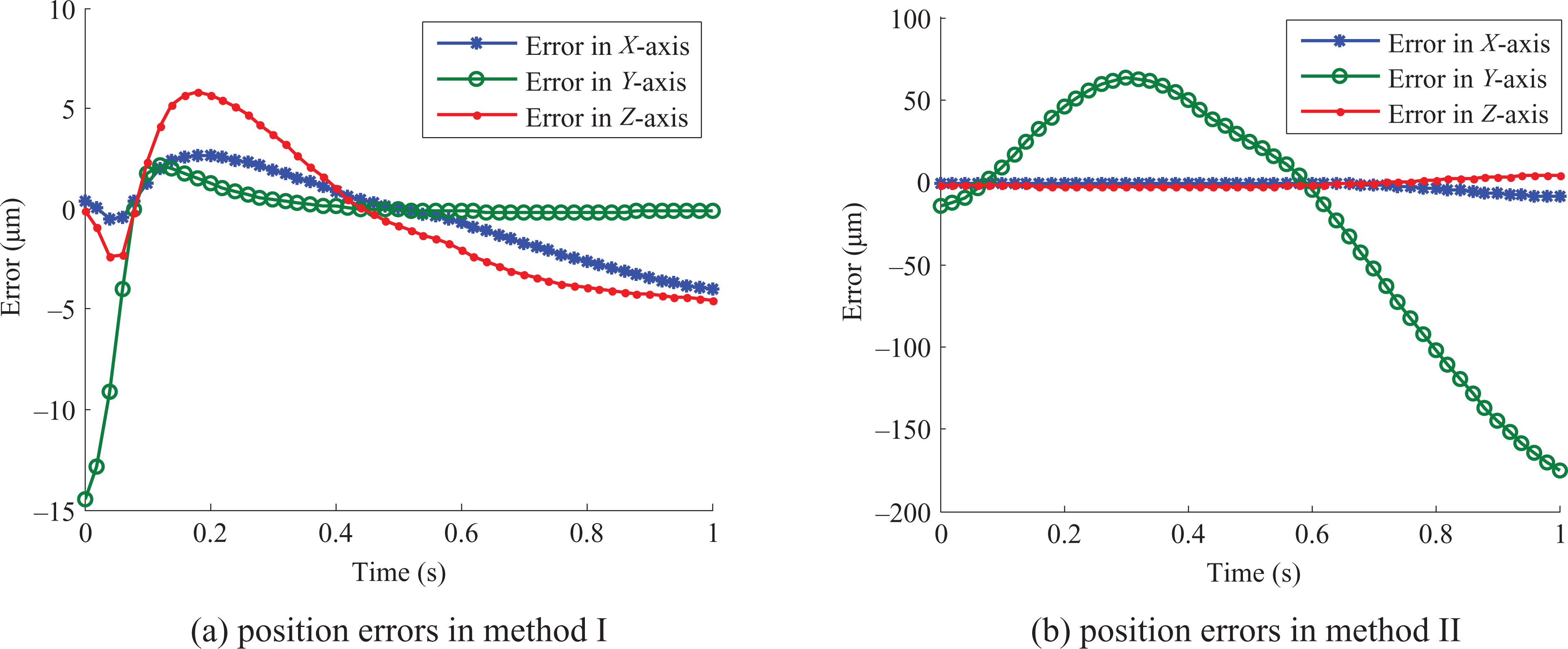Furthermore, the total position error of the tool tip ( $\sqrt{δ x_{t}^{2} + δ y_{t}^{2} + δ z_{t}^{2}}$ ) is computed, as shown in Figure 12. The comparison of the two methods reveals that it is actually effective to use an optimization method I to improve the position accuracy of the tool tip of redundantly actuated parallel manipulator.

Figure 11.

Position errors of tool tip caused by the link deformation.

Figure 12.

Total position error of two methods.

To validate the dynamic model further, the dynamic model is incorporated into the proposed control system. The control system is simulated using the Simulink soft pack in Matlab, R2014a. When the manipulator moves along the trajectory as shown in Figure 8, the control system with force optimization method I is simulated. Furthermore, the force optimization method II is used in the control system and the manipulator moves with the same trajectory. The motion error of the redundant parallel manipulator is shown in Figure 13, and it can be noted that the position error simulated from the control system is larger than that computed from the dynamic model by comparing Figure 13 with Figure 11, and the reason is that the error from the control system is not considered in Figure 11. As shown in Figure 13, when method I is used, the position error is still smaller than the error obtained while using method II.

Figure 13.

Motion accuracy of the parallel manipulator.

The total motion accuracy of the manipulator is shown in Figure 14. When method I is used, the maximum value of total position error is less than 0.031 mm, while the maximum value of total position error is greater than 0.15 mm when method II is used. In most of the motion trajectory, the total position error of the tool tip is smaller when method I is used. This result shows that the dynamic model and force optimization method are effective in control model.

Figure 14.

Total motion error of tool tip.

Conclusions

We studied the dynamic modeling of a novel 3-DOF redundantly actuated parallel manipulator by taking both the axial and bending deformations of the limbs into account. The driving force optimization method, which aims to minimize the error of the tool tip, is studied. The dynamic model is used in the model-based control system of the parallel manipulator, and the maximum position error is about 0.031 mm. When the traditional method to minimize the normal driving forces is used in the control system, the maximum position error of the tool tip is greater than 0.15 mm. The analyses and comparison reveal that the dynamic model and optimization presented in this article are effective and can be used in the control system to improve the position accuracy of the redundantly actuated parallel manipulator.

Footnotes

Declaration of conflicting interests

The author(s) declared no potential conflicts of interest with respect to the research, authorship, and/or publication of this article.

Funding

The author(s) disclosed receipt of the following financial support for the research, authorship, and/or publication of this article: This work is supported by the National Natural Science Foundation of China (grant no. 51275260) and the Science and Technology Major Project-Advanced NC Machine Tools & Basic Manufacturing Equipment (2015ZX04001002).

References

Tang

Shao

. Trajectory planning and tracking control of a multi-level hybrid support manipulator in FAST. Mechatronics 2013; 23(8): 1113–1122.

Tang

Wang

Zhang

. On the analysis of active reflector supporting mechanism for large spherical radio telescope. Mechatronics 2004; 14(9): 1037–1053.

Dongsu

Hongbin

. Adaptive sliding control of six-DOF flight simulator motion platform. Chin J Aeronaut 2007; 20(5): 425–433.

Wang

. A control strategy of a two degrees-of-freedom heavy duty parallel manipulator. J Dyn Syst Meas Control 2015; 137(6): 061007.

Chen

Wang

. Dynamic load-carrying capacity of a novel redundantly actuated parallel conveyor. Nonlinear Dyn 2014; 78(1): 241–250.

Kock

Schumacher

. A parallel xy manipulator with actuation redundancy for high-speed and active-stiffness applications. In: Proceedings of the 1998 IEEE international conference on robotics and automation, Vol. 3, Leuven, Belgium, 16–20 May 1998, pp. 2295–2300. IEEE. Available at: http://ieeexplore.ieee.org/document/680665/media.

Muller

. Internal preload control of redundantly actuated parallel manipulators-its application to backlash avoiding control. IEEE Trans Robot 2005; 21(4): 668–677.

Garg

Nokleby

Carretero

. Wrench capability analysis of redundantly actuated spatial parallel manipulators. Mech Mach Theory 2009; 44(5): 1070–1081.

Wang

. Dynamics and control of a planar 3-DOF parallel manipulator with actuation redundancy. Mech Mach Theory 2009; 44(4): 835–849.

10.

Zhao

Gao

. Development of 6-dof parallel seismic simulator with novel redundant actuation. Mechatronics 2009; 19(3): 422–427.

11.

Kang

. An inverse dynamic model of over-constrained parallel kinematic machine based on Newton–Euler formulation. J Dyn Syst Meas Control 2014; 136(4): 041001.

12.

Dasgupta

Mruthyunjaya

. A Newton-Euler formulation for the inverse dynamics of the Stewart platform manipulator. Mech Mach Theory 1998; 33(8): 1135–1152.

13.

Di Gregorio

Parenti-Castelli

. Dynamics of a class of parallel wrists. J Mech Des 2004; 126(3): 436–441.

14.

Tsai

. Solving the inverse dynamics of a Stewart-Gough manipulator by the principle of virtual work. J Mech Des 2000; 122(1): 3–9.

15.

Wiens

Shamblin

. Characterization of PKM dynamics in terms of system identification. P I Mech Eng K-J Mul 2002; 216(1): 59–72.

16.

Nahon

Angeles

. Real-time force optimization in parallel kinematic chains under inequality constraints. IEEE Trans Robot Autom 1992; 8(4): 439–450.

17.

Cheng

Yiu

. Dynamics and control of redundantly actuated parallel manipulators. IEEE/ASME Trans Mechatron 2003; 8(4): 483–491.

18.

Liu

Yao

. Control-faced dynamics with deformation compatibility for a 5-DOF active over-constrained spatial parallel manipulator 6PUS–UPU. Mechatronics 2015; 30: 107–115.

19.

Yao

Zhao

. Inverse dynamics and internal forces of the redundantly actuated parallel manipulators. Mech Mach Theory 2012; 51: 172–184.

20.

Feynman

Leighton

Sands

. The Feynman lectures on physics, vol. 2: Mainly electromagnetism and matter. Reading: Addison-Wesley. 1979.

21.

Vukovich

. Position and force control of flexible joint robots during constrained motion tasks. Mech Mach Theory 2001; 36(7): 853–871.

22.

Kock

Schumacher

. Control of a fast parallel robot with a redundant chain and gearboxes: experimental results. In: Proceedings of the IEEE international conference on robotics and automation, ICRA’00, Vol. 2, San Francisco, CA, 24–28 April 2000, pp. 1924–1929. IEEE. Available at: http://ieeexplore.ieee.org/document/844876/?arnumber=844876

23.

Shi

Yang

. Composite neural dynamic surface control of a class of uncertain nonlinear systems in strict-feedback form. IEEE Trans Cybernet 2014; 44(12): 2626–2634.

24.

Shi

Yang

. Composite fuzzy control of a class of uncertain nonlinear systems with disturbance observer. Nonlinear Dyn 2015; 80(1–2): 341–351.

25.

Zheng

Luh

JYS

. Optimal load distribution for two industrial robots handling a single object. J Dyn Syst Meas Control 1989; 111(2): 232–237.

26.

Nahon

Angeles

. Optimization of dynamic forces in mechanical hands. J Mech Design 1991; 113(2): 167–173.

Dynamic model of a 3-DOF redundantly actuated parallel manipulator

Abstract

Keywords

Introduction

Kinematics

Structure description and inverse kinematics

Velocity analysis

Dynamic model of the parallel manipulator

Acceleration analysis

Dynamic model

Driving force optimization

Deformations of non-redundant links

Platform displacement caused by the link deformation

Objective function

Control application

Control scheme

Results

Conclusions

Footnotes

Declaration of conflicting interests

Funding

References