
Abstract
A novel Udwadia–Kalaba approach for redundant parallel manipulator dynamics is presented in this article. This methodology is explicit and simple which is suitable for systems with holonomic or non-holonomic constraints. As parallel manipulator is a closed-loop mechanism, it is complex to build the dynamical model, especially for redundant parallel manipulators. This article is the first to apply Udwadia–Kalaba equation to the dynamics modeling of the redundant actuation system. In this article, we segment the parallel manipulator into several subsystems and cluster them together due to kinematic constraints. Based on Udwadia–Kalaba approach, we can establish both the direct dynamical model and inverse dynamical model of the 2-degrees of freedom redundant parallel manipulator concisely and explicitly. We use MATLAB to carry on the numerical simulation and the analysis, the results show that the approach is feasible and reliable for the 2-degrees of freedom redundant parallel manipulator.
Introduction
Generally, parallel manipulators have potential advantages of high stiffness, high accuracy, low inertia, and high payload due to their closed-loop kinematic chain mechanism. Parallel manipulators have become an active research due to these advantages. A parallel manipulator can be divided into two parts, one fixed on the base and the other move in the workspace. 1
The parallel actuated manipulator was introduced by Stewart, 2 which was first developed by Gough for the purpose of testing tires. 3 Over the past decades, many researchers and industries have paid attentions on the parallel manipulators. They can be found in many technical applications, such as simulators, 4 pick-and-place operations, 5 solar tracker, 6 telescopes, 7 medical equipment, 8 and machine tools.9–11
During the research of parallel manipulators, people exploited many new structures. In Flavio and Ron, 12 a study of the effect of including redundant actuators on the existence of force-unconstrained configurations for a planar parallel layout of joints was presented. Li and Xu 13 proposed a new 3-degrees of freedom (3-DOF) translational parallel manipulator with fixed actuators, and analyzed the manipulator by resorting to reciprocal screw theory in Li and Xu. 14 For enlarging workspace and avoiding singularities, a double parallel manipulator has been designed in 1999. 15 J. Wu et al. 16 constructed a symmetrical 3-DOF parallel manipulator with one and two additional branches, respectively, and compared their optimum performance, and proved that it is better to develop the parallel manipulator by adding only one additional leg to construct a symmetrical architecture in Wu et al. 17
The studied parallel mechanisms are commonly 6-DOF which all based on the Stewart platform. However, 6-DOF is not necessarily required in many situations. Therefore, the limited DOF manipulators are attracted by many people due to the advantages of reducing the total cost of the device while meeting the requirement of people. Redundancy can be classified as kinematic redundancy and actuation redundancy; in this article, the 2-DOF manipulator is a redundancy actuation parallel manipulator. S Kock et al. have proved that the actuation redundancy can be exploited for active stiffness and offers some good benefits for improving the behavior of parallel manipulators and optimizing force transmission in Kock and Schumacher. 18 WW Shang and colleagues19–21 did many contributions to the research of 2-DOF planar parallel manipulators.
Dynamics modeling and analysis play an important role in the study of parallel manipulators. Some classic approaches have been adopted, such as Newton–Euler approach and Lagrangian approach. In Li et al. 22 and Dasgupta and Mruthyunjaya, 23 the inverse dynamics formulation was obtained by the Newton–Euler approach. And the dynamics problem was solved using Lagrangian technique in Pang and Shahinpoor 24 and Murray et al. 25
Several new approaches have also been developed for the dynamics modeling of parallel manipulators. S Staicu et al. adopted the novel recursive matrix method to derive the kinematics and the dynamics equations of a half parallel manipulator in Staicu et al. 26 J Wu et al. 27 obtained the redundantly actuated parallel manipulator’s inverse dynamics using the virtual work principle, and the driving force was optimized by least-square method. The Lagrange–D’Alembert formulation was used in Cheng et al., 28 which developed a simple and straightforward approach to obtain the dynamical model and proved by four basic control algorithms. Z Gao et al. 29 proposed a new artificial intelligence approach to build the inverse dynamical model. Cross-coupling approach was used in Sun et al. 30
The approaches mentioned above are well applied to the parallel manipulator. However, they are all based on the D’Alembert’s Principle that is the virtual displacement principle as their start point which means that the constraint forces are assumed as ideal constraints and the total work done by the constraint forces under virtual displacement is always zero. For constrained mechanical systems, the use of Lagrangian multipliers can be effectively utilized for constraint calculation. However, it is often very difficult to find the Lagrangian multiplier to obtain the explicit motion equations for systems with a large number of DOF and also for redundant parallel manipulators. The ideal constraints assumption works well in many conditions but it is not applicable when the constraints are non-ideal.
For the reasons above, we adopt a novel Udwadia–Kalaba approach31–34 to obtain the dynamics equation of the 2-DOF redundant parallel manipulator in this article. Udwadia–Kalaba methodology does not differentiate between holonomic and non-holonomic constraints, and also does not need to determine the Lagrangian multiplier which is often very difficult to obtain. The expression is general, explicit, and simple. During the process of this approach, the unconstrained system’s motion equations are first be obtained by Lagrangian mechanics or Newtonian mechanics in terms of the generalized coordinates. Then, constraint equations are written in the form of second-order equation. Third, the constrained system’s dynamics equation can be obtained by imposing the additional generalized forces on the unconstrained system. Based on the obtained dynamical model, constraint following control can be realized and the constraint force can be obtained by Udwadia–Kalaba equation. Because Udwadia–Kalaba equation is concise and explicit, the approach has been used by many researchers.35–37 However, the approach has not been used in the redundant parallel manipulator. In fact, redundant actuation parallel manipulators are very common in the research area. It is the first time to apply Udwadia–Kalaba equation to the dynamics modeling of the redundant actuation parallel manipulator.
In this article, we first introduce the Udwadia–Kalaba equation and distinguish between direct dynamics and inverse dynamics. Second, we establish the dynamical model of the unconstrained parallel manipulator; in this process, we segment it into several subsystems and then put them together due to the constraints in the common joint. Third, we analyze both the direct dynamics and inverse dynamics of the parallel manipulator using Udwadia–Kalaba approach. In the end, we prove the feasibility and reliability of the approach by simulation.
The Udwadia–Kalaba equation
In this section, we deal with the fundamental equation of the marvelous Udwadia–Kalaba theory. The theory can be divided into three steps. 32
First, we analyze the unconstrained mechanical system which has n generalized coordinates

with the initial conditions

where

Second, a set of structure constraints and control constraints exist in the mechanical system. These constraints may include holonomic constraint, non-holonomic constraint, scleronomic constraint, or even the combination of all these constraints. Now, we assume that the system is subjected to h holonomic constraints

and s non-holonomic constraints

Under the assumption that equations (4) and (5) are sufficiently smooth and consistent, we can obtain the constraint equations by differentiating holonomic constraints (equation (4)) twice and differentiating non-holonomic constraints (equation (5)) once with respect to time t, respectively, given by

where
Remark 1
As we know, constraint equations used in Lagrange’s motion equation, Maggi equation, Boltzmann and Hamel equation, Gibbs and Appell equation, and so on, are either in the zero-order (4) or first-order (5) form. However, Udwadia and Kalaba first convert constraints into a second-order form, which is believed to be a critical step. For system’s constraint equations to be linear in accelerate, it is believed to be useful for further dynamics analysis. Thus, Udwadia–Kalaba equation is developed based on second-order constraints. It is also uncoupled and free from Lagrangian multipliers.
Remark 2
The differentiation of constraints could not result in the loss of information. In fact, the initial conditions of state satisfy the zeroth-order or holonomic constraints means the missing information is retained in initial conditions. And it has been demonstrated by stabilization, trajectory following, optimality, and other control problems. 39
Finally, the motion equation of constrained mechanical system can be acquired by combing the unconstrained motion equation (1) and the constraint equation (6). Additional “generalized forces of constraints” is imposed on the system. Thus, the actual motion equation of the constrained system can be written as

where
In Lagrangian mechanics,

where
Udwadia and Kalaba have proved the ideal constraint force

and the non-ideal constraint force

where the matrix
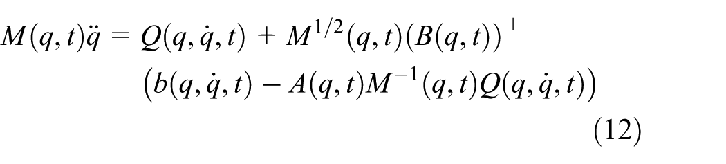
From equations (7)–(10), the general “explicit” equation of motion is (including both ideal and non-ideal constraints)

If the work done by constraint forces under the virtual displacement is zero, then
Remark 3
Udwadia–Kalaba motion equation of constrained mechanical system is applicable for holonomical and/or non-holonomical constrained systems, as well as constraints are ideal or non-ideal. We can see clearly that the equation is general, novel, concise, and simple; what’s more, there is no need to determine the Lagrangian multiplier which is often very difficult to obtain. Based on equation (8), we can get the control input
Parallel manipulator
A planar parallel manipulator is generally composed of three independent chains with one end of the chain connected to a fixed base and the other end connected to a common moving point. Depending on the kind of joints in the chain, it can be classified as RRR, RPR, PPP (P, prismatic; R, rotating), and so on. 40
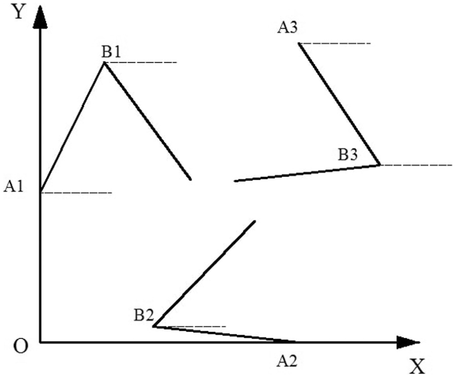
In this article, we research the RRR parallel manipulator as shown in Figure 1; a reference frame is established in the workspace. This parallel manipulator comprised three chains which are two-link mechanisms. It is actuated by three servo motors located at the base A1–A3, and the end-effector is mounted at the common joint O where the three chains meet.

Coordinates of the 2-DOF redundant parallel manipulator.
The main idea of using Udwadia–Kalaba approach for dynamics analysis is to divide the parallel closed-loop manipulator system into several open-loop subsystems. And then establish the kinematics constraints at the common joint position. The steps of this parallel manipulator’s dynamics modeling are as following
Analyze the structure of parallel manipulator system. Then make a proper segmentation at the point of O to divide it into three subsystems which only contain two-link mechanism. The proper segmentation is shown in Figure 2.
Obtain the motion equations of each “unconstrained” subsystem using Lagrangian approach or Newton–Euler approach.
Establish the kinematic constraints among the subsystems at the common joint. The constraints must be converted into the form of equation (6).
Combine the subsystems into a closed-loop mechanism and form the explicit motion constraint equation using Udwadia–Kalaba equation.
Segmentation of the 2-DOF redundant parallel manipulator.
Direct dynamics
The direct dynamics problem is to determine the motion of the system when external loads and actuator forces/torques are specified. According to Figure 2 we perform the segmentation; the unconstrained parallel closed-loop manipulator is divided into three subsystems. Then, the motion equations of the three subsystems can be easily written in the form of 41

where
The equations of motion of the “free-of-constraint” platform can be expressed by

According to Udwadia–Kalaba equation, the direct dynamics can be established as

where

Inverse dynamics
For the inverse dynamics problem, what we should do is to determine the force and/or torque applied by the actuators when the motions of manipulator are specified.
According to Udwadia–Kalaba equation, the inverse dynamics can be established as

Dynamics modeling of the parallel manipulator platform
In this section, we show in detail how to use Udwadia–Kalaba approach to obtain the dynamic characteristics of the 2-DOF parallel manipulator.
Dynamics modeling of the unconstrained subsystems
We first derive the motion equations of the “unconstrained” subsystems.
Consider subscript i = 1, 2, 3 are adopted to represent the ith chain. Ai represents the ith active joint whose coordinate is denoted by
In view of our research, object is a planar parallel robot; we can ignore the influence of gravity and further ignore the effect of each joint friction. We can adopt the standard Lagrangian approach to obtain the following equation 20

Let

where

According to the dynamics equations obtained above, we can derive the equations of motion of the unconstrained 2-DOF planar parallel manipulator as

where

Dynamics modeling of the whole open-chain system
Put three dynamical models of two-link mechanism together, and we can get the dynamical model of the unconstrained whole open-chain system

where

In the matrixes above,
Second-order kinematic constraints
Based on the dynamical model of the whole open-chain system (19), consider the constraints at the end-effector of the whole open-chain system, there exists constraint forces between each chain of the parallel manipulator.
Assume that the coordinate of the active joints is
For the relationship between the first open chain and the second open chain, we get
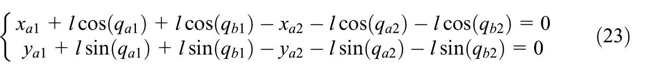
Taking the time derivative twice, we get

For the relationship between the first open chain and the third open chain, we get

Taking the time derivative twice, we get

There are two additional constraint equations which are used to constraint the trajectory of the point O, which is the same point of three chains. The trajectory is a straight line parallel to the x coordinate.

Convert the coordinate of point O to the angle of the first two-link mechanism’s active joint and passive joint (

Taking the time derivative twice, we get

Then, combine equations (24), (26), and (29), the constraints can be written in the form of equation

where

Dynamic characteristic and numerical simulation
Equation of motion with constraints
In “Dynamics modeling of the parallel manipulator platform,” we have obtained the dynamical model and kinematic constraints of the parallel manipulator; now, we impose the additional “constraint forces” on the unconstrained system. Thus, form the explicit equation of motion with the following constraints

where

According to Udwadia–Kalaba equation, the constraint force that is the inverse dynamics of the parallel manipulator can be written in the form

where the superscript ‘+’ denotes the Moore–Penrose generalized inverse.
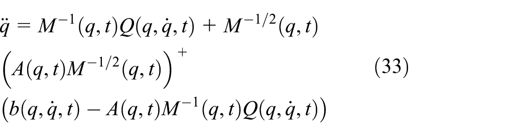
From equations (31) and (32), the general equation of motion (the direct dynamics of the parallel manipulators) is
Remark 4
Shang et al. 19 have obtained the dynamics equation of the 2-DOF redundantly parallel manipulator by Lagrangian dynamics. During the process, the Lagrangian multiplier is difficult to be measured directly and calculated by linear projection method. However, there is no need to make any linearization or approximations by the Udwadia–Kalaba approach. Exact analytical solutions to the tracking control of mobile robots are obtained. In Udwadia–Kalaba equation, all the variables are easy to get.
Parameters and initial conditions
We have obtained the motion equations of this manipulator by the dynamics analysis before. Now, we are going to verify the validity of the theory by numerical simulations. The numerical integration through-out this article is done by MATLAB. In this section, the numerical simulation results and analysis are shown.
The coordinates of three bases, the links’ length, mass, mass center, and rotational inertia are known.19,21 Through the computational formula of dynamic parameters (17), we can obtain the value of dynamic parameters
Parameter values of the system.

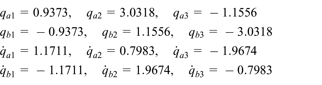
The initial states include each chain’s initial angle and initial angular velocity. Initial coordinate of the point O is
Numerical simulation results and analysis
With the equations and initial conditions, we can solve the problem of the parallel manipulator’s dynamics including direct dynamics and inverse dynamics. Figures 3–13 show the direct dynamic characteristics, and Figures 14–16 show the inverse dynamic characteristics of the redundant parallel manipulator.
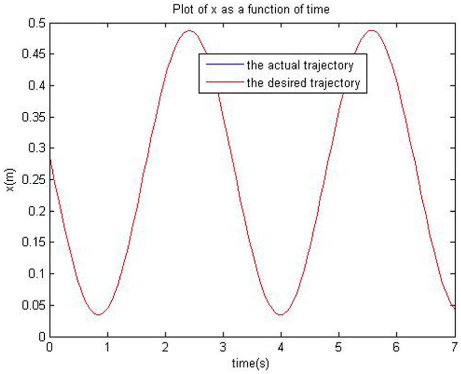
x-coordinate curve of the point O.

y-coordinate curve of the point O.

Angle curve of active joint angle qa1 and passive joint angle qb1.

Angle curve of active joint angle qa2 and passive joint angle qb2.
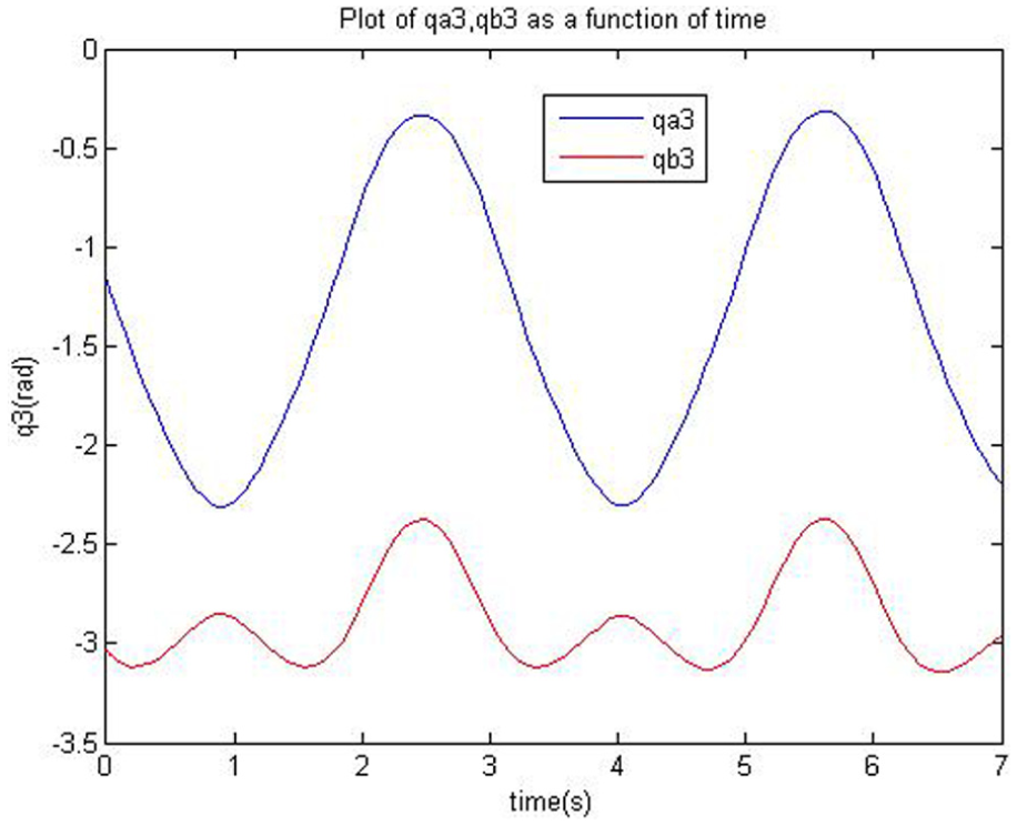
Angle curve of active joint angle qa3 and passive joint angle qb3.
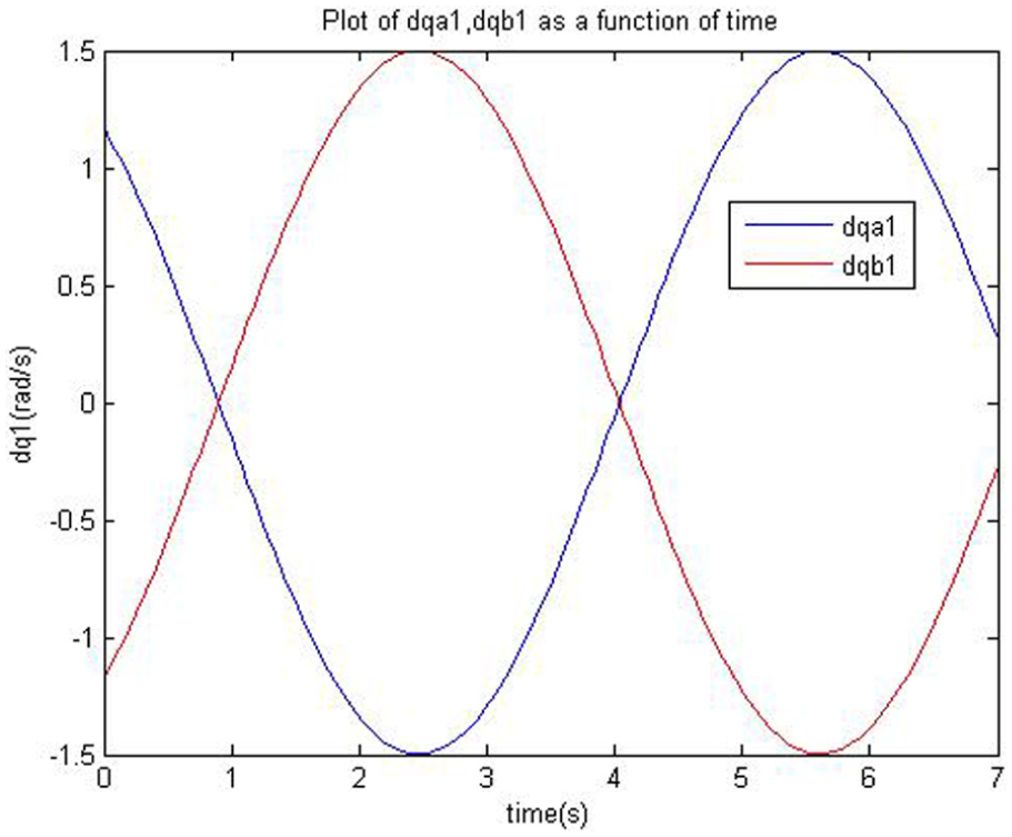
Angular velocity curve of active joint angle qa1 and passive joint angle qb1.
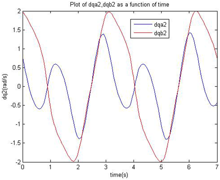
Angular velocity curve of active joint angle qa2 and passive joint angle qb2.
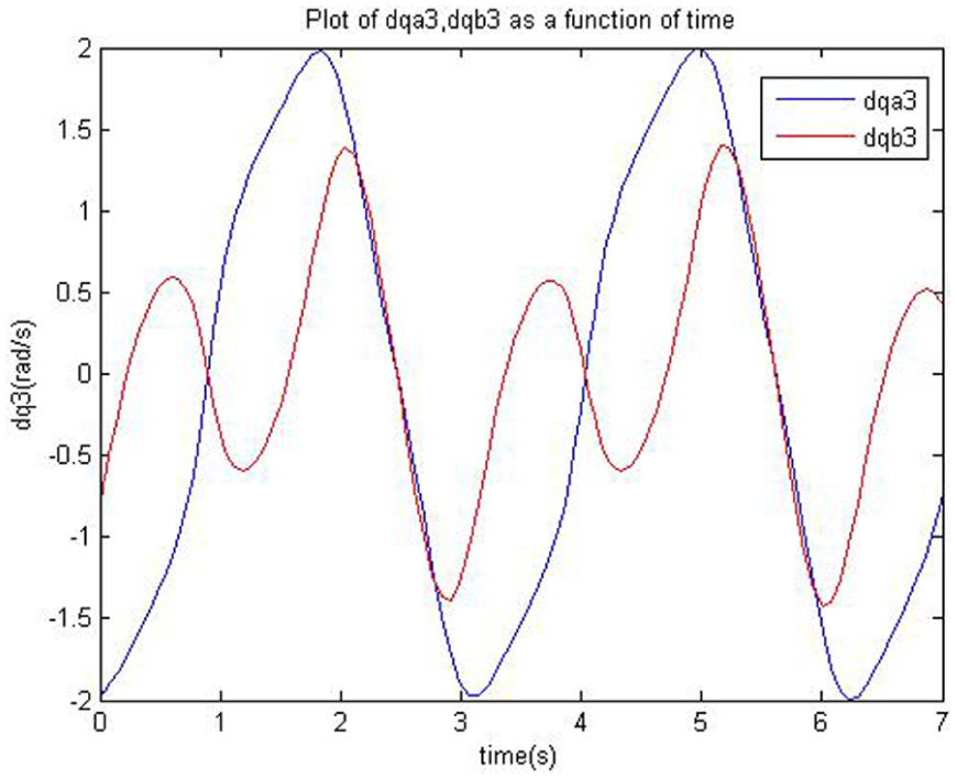
Angular velocity curve of active joint angle qa3 and passive joint angle qb3.
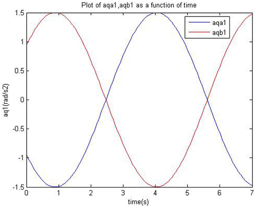
Angular acceleration curve of active joint angle qa1 and passive joint angle qb1.
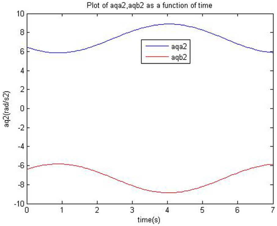
Angular acceleration curve of active joint angle qa2 and passive joint angle qb2.

Angular acceleration curve of active joint angle qa3 and passive joint angle qb3.

Torque curve of active joint A1 and passive joint B1.

Torque curve of active joint A2 and passive joint B2.
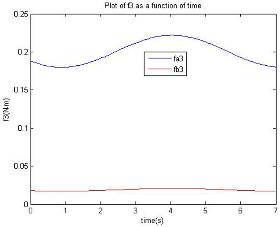
Torque curve of active joint A3 and passive joint B3.
Figures 3 and 4, respectively, show the actual and desired x-coordinate curve and y-coordinate curve of the point O as a function of time. It is clear to see that the actual trajectory coincides well with the desired trajectory.
The angle curves of each active joint and passive joint are shown in Figures 5–7. In Figure 5, the first chain’s angles of the active joint and the passive joint are in accordance with the constraints expressed in equation (28). From Figures 6 and 7, we can see that the angles of the second and third chains are also changed in periodic, but the period time is half of the first chain which is consistent with actual.
Figures 8–10 show the angular velocity curves of each active joint and passive joint. Figure 8 shows the first chain’s angular velocity which is in accordance with the constraints derived from equation (28). The angular velocity of the second and third chains is also in a period which is half of the first chain.
The angular acceleration curves of each active joint and passive joint are shown in Figures 11–13. The angular acceleration of the first chain meets requirement expressed in equation (29). In Figures 11–13, the angular acceleration of active joint is opposite to the angular acceleration of passive joint.
Figures 14–16 expressed the torque curve of each active joint and passive joint. We can see that the active joint’s torques fa1, fa2, and fa3 changed in period, the passive joint’s torques fb1, fb2, and fb3 are also in a same periodic change and it is close to zero. These results satisfy the requirements that driving torque of the passive joint is zero.
From Figures 3–16, it is obvious to find that this approach expressed the performance of the parallel manipulator and all performance meets the theoretical expectation.
Conclusion
The main reason for studying closed-loop parallel manipulators is that it has the advantage of high precision, high stiffness, high payload, and low inertia, so they have broad application prospect. Different from other approaches, Udwadia–Kalaba approach presents a novel, concise, and explicit motion equation for constrained mechanical system which is uncoupled and free from the Lagrangian multiplier. There is no need to make any linearization or approximations by Udwadia–Kalaba approach. We can easily get the exact analytical solutions for all the variables. This approach is suitable for systems with holonomic and/or non-holonomic constraints, as well as constraints are ideal or non-ideal. This article is the first to apply Udwadia–Kalaba approach to the redundant actuated system.
In this article, we present a novel Udwadia–Kalaba approach for the dynamics modeling of the 2-DOF redundant parallel manipulator, including direct dynamics and inverse dynamics. The expression of the method is general, simple, and precise. First, the fundamental equation of the marvelous Udwadia–Kalaba theory is introduced. Second, we describe the direct dynamics and inverse dynamics of the parallel manipulator and establish its dynamical model. Then, we use Udwadia–Kalaba approach to analyze both the direct dynamics and inverse dynamics of the closed-loop 2-DOF redundant parallel manipulator, and the simulation is done by MATLAB. The results show that the approach is feasible and reliable.
Footnotes
Academic Editor: Aditya Sharma
Declaration of conflicting interests
The author(s) declared no potential conflicts of interest with respect to the research, authorship, and/or publication of this article.
Funding
The author(s) disclosed receipt of the following financial support for the research, authorship, and/or publication of this article: This research was supported by National Natural Science Foundation of China (no. 51505116), Natural and Science Foundation of Anhui Province (no. 1508085SME 221), the Fundamental Research Funds for the Central Universities (JZ2016HGTB0716) and China Postdoctoral Science Foundation (2016M590563).