Sage Journals: Discover world-class research

Abstract

Tool wear monitoring using vibrations is a complex task, due to various simultaneously occurring vibration sources and due to distortion of the signals acquired. This work investigates the mechanism by which tool wear information is concealed within acquired process-intrinsic vibration signals. Excluding other sources of vibration, such as machine-related, is attempted utilizing process simulations. As a case study, face milling is performed for three different cutting speeds. At first, the resulted simulated wear curves have been compared with experimental ones resulted under the same cutting conditions. Then, a quantification of the effect of tool wear on the acquired signals is presented.

Keywords

Tool wear finite element method monitoring vibrations wear curves

Introduction

Tool wear is the phenomenon of the gradual deterioration of cutting tools due to regular operation. It is a significant topic of interest for manufacturing industries, as they need to utilize the full potential of each cutting tool, thus increasing their productivity.¹ Predicting tool wear level is also crucial to industry,² as it can be used to give information on the remaining service life of the tool, minimizing downtime, and eliminating scrap parts due to tool failure during machining. Therefore, online monitoring and estimation of tool wear in machining processes, is a significant research task.³ Process signals, such as vibrations or current, can be correlated with tool wear evolution and utilized for online monitoring of a machining process. For instance, vibration signals can be acquired⁴ utilizing appropriate sensor systems and be correlated with corresponding tool wear levels employing signal processing methods. However, due to various mechanisms, the signal is distorted and the information is “hidden” among noise and other pieces of information.⁵ Papacharalampopoulos et al.⁶ have showcased how the propagation of elastic waves affects the process signal and in Teti et al.,⁷ the effect of non-desired oscillations on signal noise is presented. Thus, employing numerical simulations of machining processes, one can isolate the process-level information (Figure 1), while checking the validity and the accuracy of the results.

Figure 1.

Decomposing information-carrying vibration.

Literature review

In the literature, many approaches have been utilized, so far, in order to estimate and model tool wear via acquired process signals, both experimentally and numerically. As it regards experimental approaches, studies try to estimate the predictability of tool wear levels in milling. Stavropoulos et al.⁵ have utilized a combination of current and workpiece acceleration measurements to predict the Taylor curve of the cutting tool. Moreover Doukas et al.⁸ experimented in face milling and tried to make a correlation between sensorial data and tool wear levels. Correlation between tool wear and the acquired signals has been estimated employing signal processing and pattern recognition techniques. Research on online monitoring of tool condition has also been conducted. Sanchez et al.⁹ have proposed an online monitoring method for tool wear, based on cutting force signals measured during the process. Ritou et al.¹⁰ proposed a cutting force monitoring system based on eddy current sensors and estimated cutter eccentricity due to worn edges, in order to predict tool failure. Analytical and experimental methods have been described and implemented, involving vibration signals and the use of three perpendicular components of cutting forces, in order to find a correlation between tool wear and signals measured from the cutting tool. Also, correlation between tool wear and vibration signals, in end milling operation, has been investigated.¹¹ Tool wear progression models have also been implemented¹² under semi-dry and dry conditions. Furthermore, audio signals¹³ and machine vision¹⁴ have been proposed as novel tool wear monitoring techniques.

Regarding data processing tools, singular spectrum analysis and cluster analysis on vibration signals has been attempted,¹⁵ Hilbert–Huang transformation was used to decompose vibration signals in both milling¹⁶ and drilling,¹⁷ and statistical analysis and artificial intelligence methods have been used for tool wear identification. In Zhu and Liu,¹⁸ a hidden semi-Markov model was employed for prediction of remaining useful life of the tool, while in Javed et al.,¹⁹ a summation wavelet-extreme learning machine ensemble with incremental learning was used to predict tool wear based on cutting force and vibration data. Hesser and Markert²⁰ retrofitted an older computer numerical control (CNC) milling machine with a vibration monitoring system and developed a neural network for wear state classification. Moreover, auto-regressive (AR) models have been utilized in industrial applications,²¹ coupled with different methods such as nonlinear dynamical approaches²² or operational modal analysis.²³ However, all these methods, being empirical, lack physical meaning and the actual correlation between tool wear development and process signals and parameters cannot be clearly defined. Consequently, there is a clear requirement for the development of a more direct and intuitive signal analysis, where, if possible, features of the signals (such as spectrum characteristics) will be directly correlated with physical phenomena. Concerning the simulations aspect, there have been previous works for predicting tool wear and tool life using finite element method simulations; Huang’s and Usui’s wear models and their experimental calibration²⁴ are an example. Usui’s model provided better results, when compared with the experiments and appeared to have better stability than Huang’s model. Other works include predicting the effects of cutting parameters caused from the variation of cutting forces on tool wear,²⁵ predicting tool wear in orthogonal cutting of Titanium alloys using finite element model (FEM) simulations,²⁶ and FEM using self-developed continuous remeshing method to form segmented chips.²⁷ Also, there have been reported works with use of Johnson–Cook model for orthogonal cutting of Ti6Al4V²⁸ and AISI 1045,²⁹ correlation of tool wear with cutting parameters during milling of Inconel 718,³⁰ and computational research on cutting edge geometries with the aim of decreasing tool wear in hard milling operations and estimation of tool stresses.³¹ Finally, forecasting tool wear progression based on FEM simulation in turning operations³² has appeared in the literature. In this last work, a coupled abrasive–diffusive wear model has been implemented in order to predict abrasive and diffusive wear evolution. The model was calibrated with experimental results. However, there are not many researches regarding acquired vibration signals from numerical simulations.

As it can be observed from the literature review, there has been significant effort toward indirect tool wear monitoring, through post-processing of different process signals. However, the mechanism(s) in which the acquired vibration signal, measured during the process, encapsulates the information related to tool wear level, is yet to be revealed. As a result, the scope of this study is to reveal these mechanism(s) and provide further understanding on the information that is carried on the vibration signals measured during the process.

Toward this goal, simulations of the milling process have been conducted. Then, a comparison has been conducted between tool wear curves acquired both experimentally and from simulations. Following, right after being pre-conditioned to be able to be processed, the acquired—through simulations—vibration signals are correlated with the tool wear level quantitatively, through AR models. The above-mentioned have been performed for different cutting speeds.

Methodology

In this section, the methodology is described within three sections as follows: the “Backbone” section deals with the specific approach, namely, how the set of simulations is defined. The “Numerical simulations” section is about modeling, and the “Tool wear curves extraction” concerns the extraction of the tool wear curves themselves.

Backbone

Driven by the fact that the environmental and the machine-related noise have to be eliminated, the vibration distortion mechanisms due to movement of the machine tool parts¹ and due to wave propagation⁶ have to be removed. On the contrary, vibration generation mechanisms such as cutting force variations, friction, and crack propagation will be taken into consideration. Factors that will affect these are as follows:

Cutting speed.

Feed-rate.

Workpiece material properties.

Depth of cut.

In order to develop the holistic empirical model, which will utilize vibration signals as input and estimate the tool wear progression as output, the milling process has to be decomposed in two levels: process level and machine level, as shown in Figure 2. Simulations have been conducted in commercial software, which is based on finite elements modeling. The whole methodology can be divided in four components (Figure 2). During the first one, the original geometry of the cutting tool is modified to represent a worn tool, based on experimental data⁵ incorporating both crater and flank wear. Second, the simulations are performed for each level of tool wear, successively, using the final stress and temperature values of the previous tool wear level as initial stress and temperature values for the next tool wear level simulation. Next, the Usui model²⁴ is used to match temporally the experimental values with the numerical values of tool wear and compare the Taylor curves.¹ Finally, the correlation analysis between the tool wear level and the numerically acquired vibration signal is performed.

Figure 2.

The methodology of the modeling extraction from simulations.

Each simulation is conducted for a time interval that is defined as the time needed for the stress and temperature values to reach an equilibrium stage, at which no variation and no increment at these measures is observed. The use of this assumption has been verified by the evolution of these measures in time as well as by Klocke et al.³³ This process of sequential simulations and the corresponding timing is shown in Figure 3; the evolving measure can be either temperature or stress level, δt refers to simulation time, t denotes actual time, and the red dotted curve corresponds to the tool wear level.

Figure 3.

Policy of estimating time as parameter.

Numerical simulations

Simulations have been conducted for three different cutting speeds equal to 210, 338, and 467 m/min. Worn tool geometry (Table 3) was simulated for each cutting speed case. The simulation model includes a single insert²⁴ and a work piece with the following dimensions: L30 mm × W2.5 mm × H5 mm. The work piece dimensions have been chosen so that a minimum number of elements would be needed for each simulation. The materials of the work piece and inserts have been defined as indicated in Table 1. The insert is Sandvik CoroMill N365-1505ZNE-KW4 1020,³⁴ and its specifications are presented in Table 2. All simulations have been conducted in 50 steps. Shear friction factor has been defined equal to 0.8,³⁵ and convective heat transfer coefficient for dry machining equal to 11 W/m² K.³⁶ The formulation method that has been used for the simulations was Lagrangian incremental method since machining operations, like face milling, include discontinuous effects, such as chip formation, and are not steady-state operations.³⁷

Table 1.

Simulation setup parameters.

	Workpiece	Insert
Number of elements	20,000	80,000
Material	CGI 450	Tungsten carbide
Initial temperature (°C)	20	20
Simulation steps	20	20
Solver-iteration	Conjugate gradient	Direct iteration
Thermal conductivity (W/m K)	38	110
Shear friction coefficient	0.8
Heat transfer coefficient (W/m² K)	11

Table 2.

Milling insert specifications.

Inscribed circle diameter (mm)	Thickness (mm)	Major cutting edge angle (°)	Material	Coating
15	5.66	65	Tungsten carbide	PVD TiAlN

Table 3.

Library with wear values.

Wear values in μm
210 m/min	338 m/min	467 m/min
0	0	0
25	25	25
50	50	50
75	75	75
90	90	90
100	100	100
120	120	120
	130

The material of the work piece that has been chosen in the FEM simulations was CGI 450. The stress and strain that the workpiece material is subjected to during machining induce elasto-plastic and plastic behavior during the chip formation. In order to accurately model the machining process, one has to account for this behavior. The FEM software that was utilized offers the power law model (equation (7)), which calculates the flow stress of the material. Because of the difficulties about estimating the model constants, an empirical calibration of the power law model, regarding the stress–strain rate values provided from Johnson–Cook model, has been implemented. Then, the c, m, and y values resulted from the model calibration have been input in the FEM software. The resulted curves of power law model in comparison with Johnson–Cook model, for different strain rate values are shown in Figure 4. The calibration procedure is shown in Appendix 1.

Figure 4.

Flow stress curves calculated from power law model.

In continuation to this, the model that has been used in order to produce the wear curves was the Usui’s wear model²⁴ (equation (1)), as it is appropriate for metal cutting operations, it is more stable than the other wear models,²⁴ and it can be easily calibrated. The specific mathematical model is described by the following equation

W = \int apV \exp (- \frac{b}{T}) dt

(1)

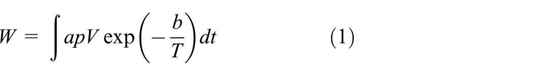
where p is the interface pressure, V is the sliding velocity, T is the interface temperature, and a and b are the experimentally calibrated coefficients.

Tool wear curves extraction

A library with specific tool wear values from previous work on CGI 450 machining,⁵ along with the time intervals, at which these values were obtained was created. Thus, the theoretical curve could be formed for each cutting speed case. This method was chosen in order to minimize the analysis time. The interface pressure and temperature values that are used in Usui’s model have been calculated through FEM simulations. After integrating equation (1), the following form of Usui’s model (equation (2)) is obtained

\begin{matrix} Δ t_{n} = \frac{w_{n} - w_{n - 1}}{α V p_{n - 1} \exp (- \frac{b}{T_{n - 1} + 273})} \\ t_{n} = t_{n - 1} + Δ t_{n} \end{matrix}

(2)

where p_i₋₁ and T_i₋₁ are the interface pressure and temperature values provided by simulations for each value of wear in the library, respectively. Finally, after calculating the time intervals, the curves have been created. The steps given above have been repeated for the three cutting speed cases (210, 338, and 467 m/min). The whole procedure is presented below with the use of a flowchart (Figure 5). The specific wear values for the library are presented in Table 3.

Figure 5.

Flowchart of the overall calibration methodology.

In order to simulate all these cases under the prism of the methodology described in section “Backbone,” a method to accelerate total simulation time has been chosen. Each insert geometry has a concave section in its rake surface that represents crater wear and a similar section in its release surface, half the wear land, as experimentally indicated, that represents flank wear. The size of its concave section has been defined according to the resulted worn inserts geometries from experiments.⁵ The first insert has no concave sections and represents the initial insert geometry with wear: w = 0 μm. The following six inserts have a slot located in their lower rake surface of depth values r = 25, 50, 75, 90, 100, and 120 μm and in case of 467 m/min, r = 130 μm. This method of design of “pre-worn” inserts has been preferred in order to drastically reduce simulation time for test cases. In Figure 6, a close-up view of crater wear is given.

Figure 6.

Concave slot on the lower rake surface of the insert.

Discussion of results

Tool wear evolution in time

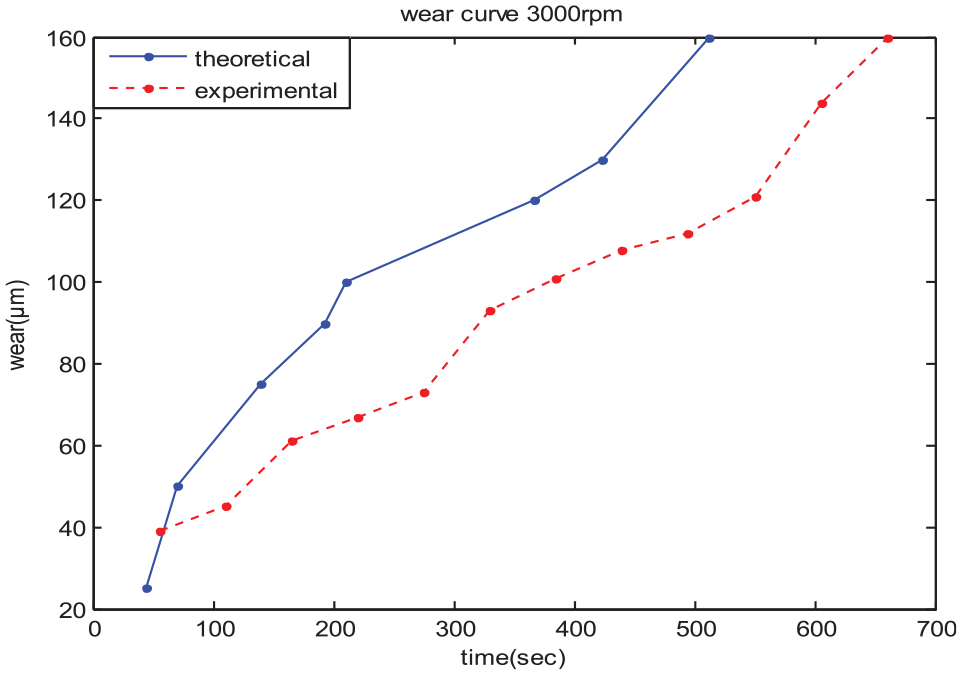
After post-processing of the simulation results (Figure 7), mean values of interface pressure and temperature have been utilized as input to the wear model. This way, coefficients a and b were calculated through calibration of the Usui model, with the wear data for 338 m/min cutting speed, solving equation (2); the resulted tool wear curves have been compared (Figures 8 –10) with the corresponding experimental form.⁵ The values that came up after this process are equal to a = 0.65 × 10⁻¹⁰ and b = 3500.

Figure 7.

Post-processing collecting FEM results.

Figure 8.

Wear progression versus time for 210 m/min.

Figure 9.

Wear progression versus time for 338 m/min.

Figure 10.

Wear progression versus time for 467 m/min.

By observing Figures 8 –10, we can see three different behaviors regarding the prediction of the tool wear values:

For the case of 210 m/min, the theoretical model underpredicts the tool wear values to a significant extent.

For the case of 467 m/min, the theoretical model slightly overpredicts the wear values. However, the slope of the theoretical curve follows the slope of the experimental.

An important observation that has to be noticed is that the resulted theoretical curves verify the theoretical wear graph; tool life decreases as cutting speed increases, according to Taylor’s equation.¹

Pre-conditioning vibration signals

The second part of this work deals with processing of vibration signals, in order to find a correlation between them and tool wear progression. So, the algorithm (Figure 11) started by acquiring the workpiece displacement signal from each simulation in the simulations software. The sampling has taken place at a point located on the specimen, where a sensor could be placed. Because of the non-uniformity of the sampling periods in each signal, an interpolation of a stepped curve has been made in the displacement data. Therefore, a displacement curve, with equal sampling periods this time, has been provided (Figure 12).

Figure 11.

Algorithm for vibration signal processing.

Figure 12.

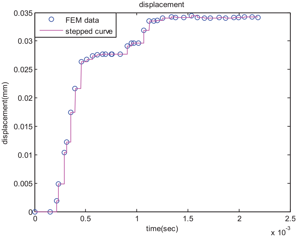
Displacement from FEM and interpolation of stepped curve.

Then, the acceleration signals of each simulation had been produced by second-order differentiation (equation (3))

a_{n} = \frac{x_{n} - 2 x_{n - 1} + x_{n - 2}}{h^{2}}

(3)

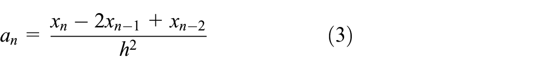
where x_i is the displacement (mm), a_i is the acceleration (mm/s²), and h is the time increment (s).

Since the magnitude of the vibration itself has been proved to be not so important in this work, in order to normalize the acceleration signal, the acceleration values were divided by the quantity $\int_{0}^{T} a^{2} dt / T$ .

Subsequently, a filter was applied in order to reduce the high-frequency variations, so the final time-domain signal was resulted (Figure 13). Finally, the spectrogram of the acquired signals was produced, so any possible (qualitative) correlation between the tool wear progression and each signal could be observed (Figure 14).

Figure 13.

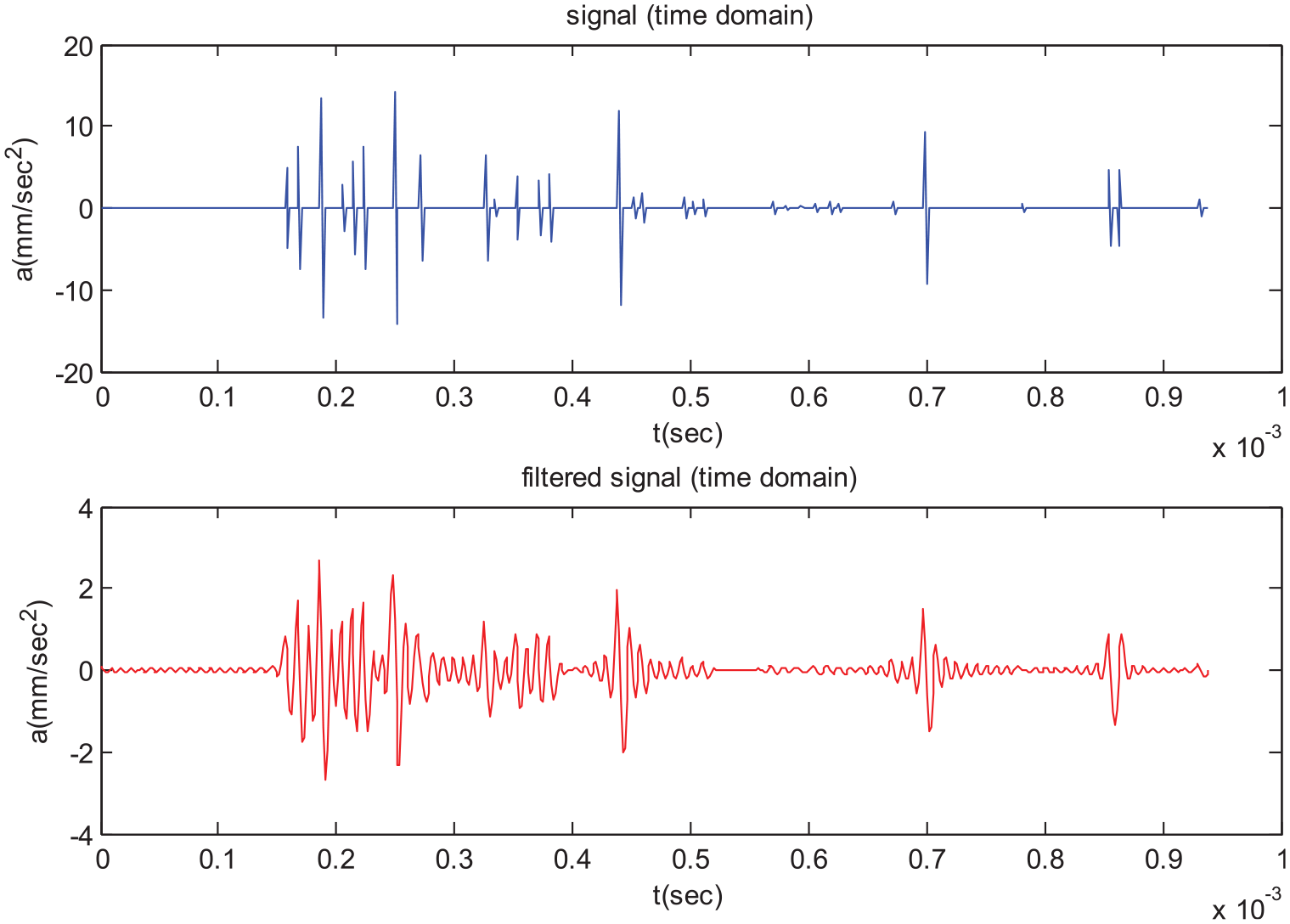
Acceleration time domain signal (top) and final acceleration time-domain signal (bottom). Unit is normalized mm/s².

Figure 14.

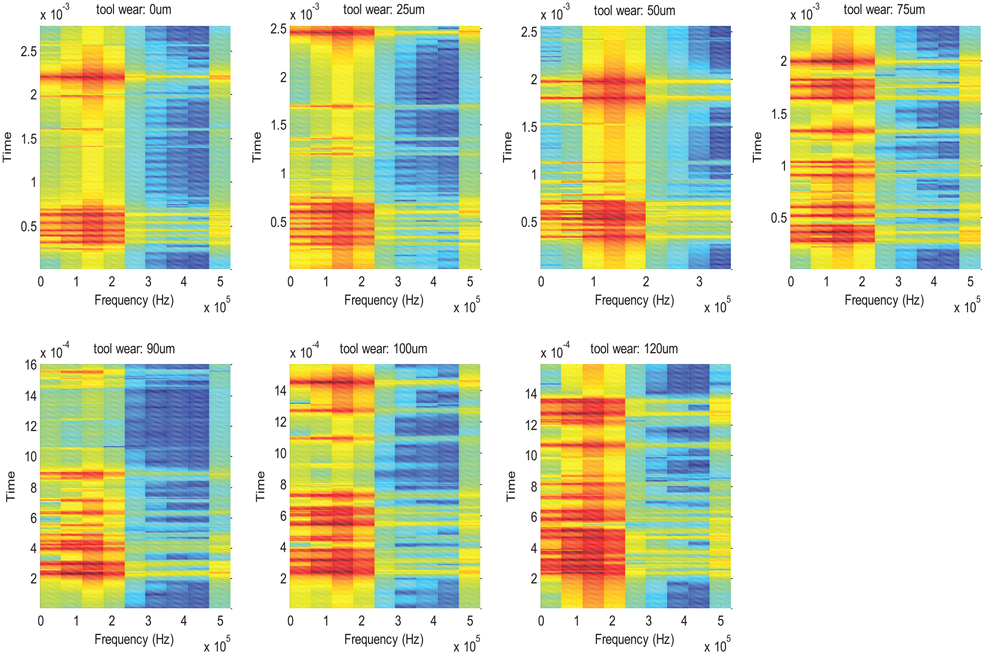
Evolution of spectrograms for 210 m/min.

Modeling using system identification meta-information

A significant observation that can be made from the corresponding spectrograms of the acquired signals is that, as tool wear increases with time, the bursts of the signals become more frequent; the occurrence of the high magnitude is notated in red color in Figure 14 and the vertical distance in the graph between these maxima becomes less as tool wear levels increase. An example of that is given below for the case of 210 m/min. This is promising for the case of real-time signal processing as the distortion of the signals due to transmission through the machine-tool elements can be predicted and thus lead to a time–frequency toolbox for identification of the tool wear level.

This correlation between tool wear level and vibration signals characteristics can be quite useful in predicting tool wear; indirect monitoring of tool wear can benefit from this technique and predictive maintenance of machine tool can be possible in low cost, without force sensors. The way the tool wear information is concealed within the vibration signal is quite complicated; however, it seems that a spectrogram could help toward tool wear prediction. The spectrogram of each signal has located in time–frequency the increased complexity (high variations) of the signal.

Also, system identification method has been implemented on the acquired vibration signals, in order to find another correlation between the signals tool wear evolution, quantitative this time. AR modeling (equation (4)) has been applied in order to identify the difference equation³⁸ which can be used to predict each acceleration signal

y (n) = - \sum_{k = 1}^{p} a_{k} y (n - k) + ε (n)

(4)

or using polynomial notation

A (L) y (n) = ε (n)

(5)

where $a_{1}$ , $a_{2}$ , …, $a_{k}$ are the parameters of the model; p is the order of the model; ε is the zero mean white noise; and L is the lag operator.

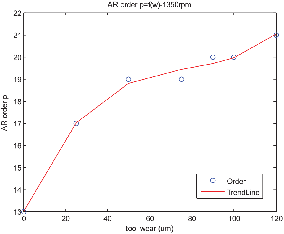
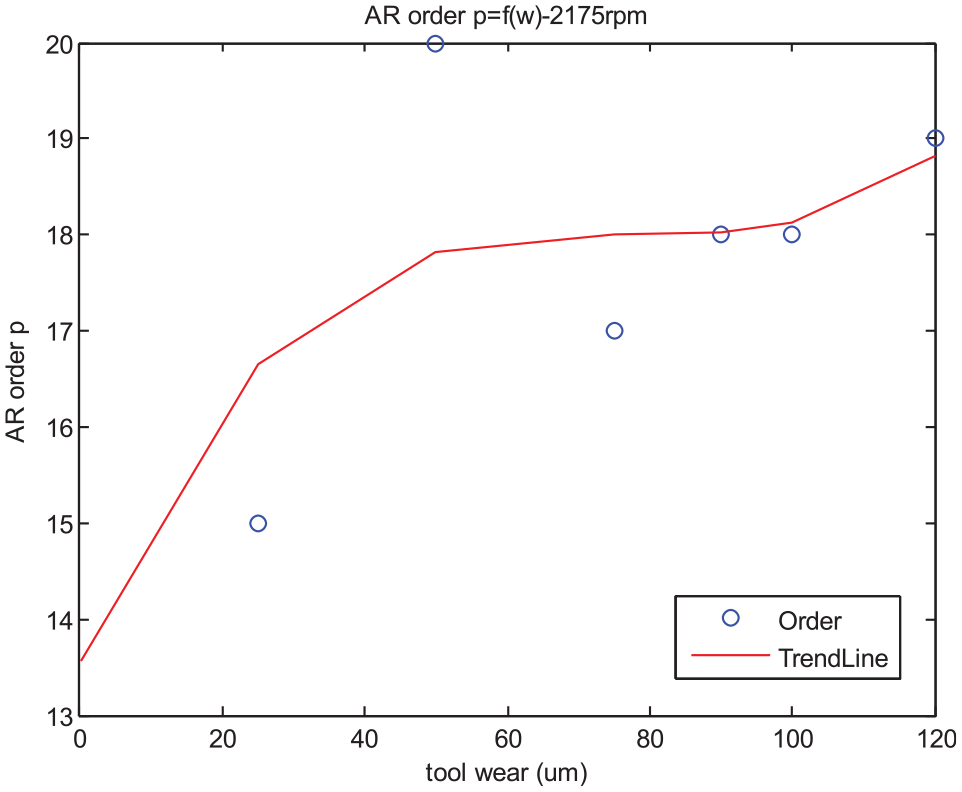
In each case of tool wear, the AR model has been implemented in order to find the minimum order p of the difference equation that forecasts with the best way the acceleration data (Figure 15). The “best way” implies the use of a criterion exploiting the error between the real and simulated signal. Therefore, the graphs (Figures 16 –18), one for each case of cutting speed, that present the relation between the minimum order p and tool wear have been produced.

Figure 15.

Signal of acceleration data and forecasted signal using AR model.

Figure 16.

Minimum order of AR model versus tool wear for 210 m/min.

Figure 17.

Minimum order of AR model versus tool wear for 338 m/min.

Figure 18.

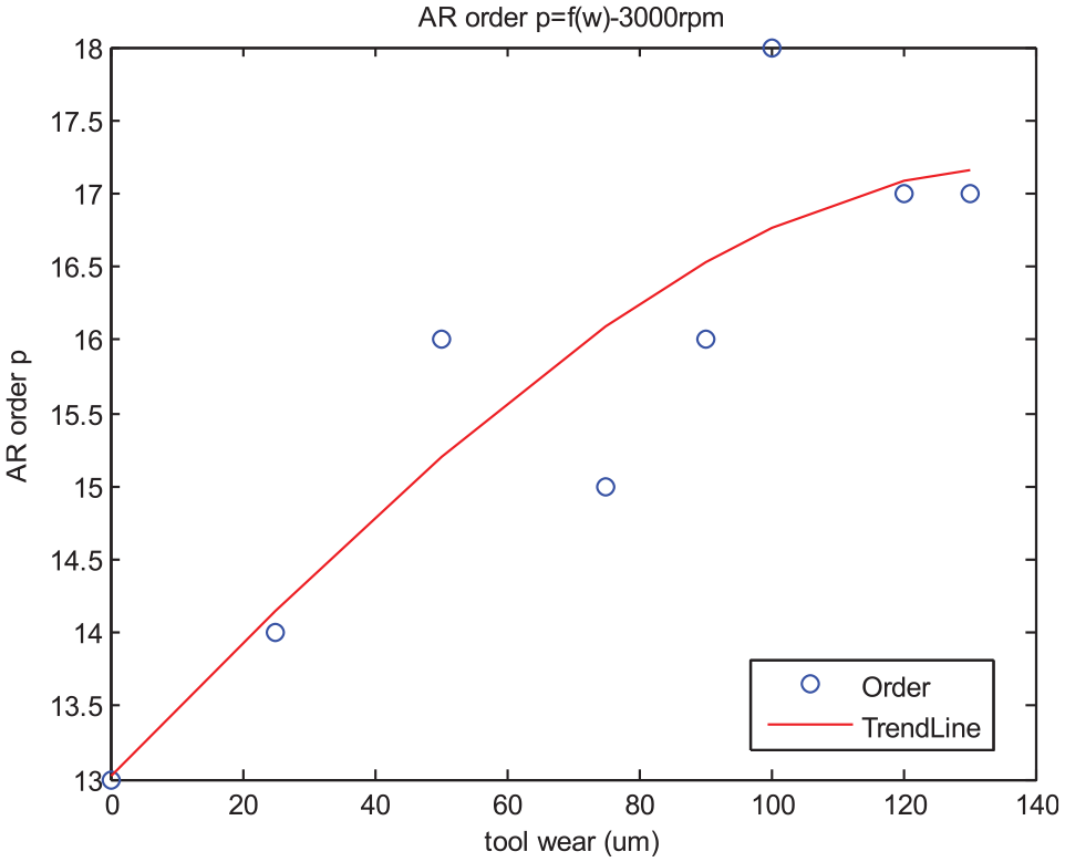
Minimum order of AR model versus tool wear for 467 m/min.

From the above figures, it can be observed that the minimum order of AR model increases as tool wear level increases. This observation agrees with the spectrograms; the duration of vibration bursts increases with the rise of tool wear. This implies that the complexity of the AR systems describing the vibration signals, as measured by their order, also increases. Also, what is observed is that in terms of mean values, the order of the systems describing vibration signals tends to be smaller as the cutting speed is increasing. Measuring complexity of a system, however, is not straightforward; the linear technique of AR modeling used here only provides an indication that systemic complexity is measurable. In reality, the “spectrogrammic content” of the signal is prone to changes, due to propagating vibrations within the machine tool (extending the conclusions of Papacharalampopoulos et al.).⁶ However, previous literature seems to verify this approach; the harmonic content of the vibrations changes with time, as per experiments.⁵

Conclusion

This article is an effort toward identifying the mechanism by which the tool wear level–related information is concealed within vibration signals, through process simulation and signal processing. According to the results that have been presented above, the following conclusions can be drawn:

Regarding the usefulness of the simulations themselves, it has been proved that the tool wear evolution can be estimated with relative success utilizing mechanics simulations and Usui’s model. As such, simulations can be considered as a basis to form digital shadows for machining.

The correspondence between vibrational data and tool wear can be approximated through time–frequency localization. The vibration signals will be for sure distorted by mechanical phenomena; however, the information of the tool wear that has been concealed within these signals seems to be highly related to complexity. This has been proved through utilization of AR modeling of the vibrations themselves. The order of the AR is highly affected by the tool wear level, and as such, this can be the basis for a successful mode.

With a quantitative relationship between the signals and the tool wear level being found, future actions can include the following:

Implementation of spectrum-related methods in conjunction with similarity metrics during signal processing, with the aim of minimization of signal distortion, due to stochastic process-related phenomena.

Statistical analysis should be performed for different cases of materials and machine tools, in order for signal characteristics (i.e. spectral density) to be able to give information on tool wear level, despite what the oscillation modes of the machine tool are and how this affects the tool wear metrics.

Machine learning techniques could be pre-trained to utilize features of vibration signals that include measuring complexity and spectrograms.

Footnotes

Appendix 1

Handling Editor: James Baldwin

Declaration of conflicting interests

The author(s) declared no potential conflicts of interest with respect to the research, authorship, and/or publication of this article.

Funding

The author(s) received no financial support for the research, authorship, and/or publication of this article.

ORCID iD

Panagiotis Stavropoulos

References

Chryssolouris

. Manufacturing systems—theory and practice. 2nd ed. New York: Springer-Verlag, 2006.

Vetrichelvan

Sundaram

Kumaran

, et al. An investigation of tool wear using acoustic emission and genetic algorithm. J Vib Control 2014; 21: 3061–3066.

Altintas

. Manufacturing automation: metal cutting mechanics, machine tool vibrations, and CNC design. Cambridge: Cambridge University Press, 2012.

Hopkins

Hosseini

. A review of developments in the fields of the design of smart cutting tools, wear monitoring, and sensor innovation. IFAC PapersOnLine 2019; 52: 352–357.

Stavropoulos

Papacharalampopoulos

Vasiliadis

, et al. Tool wear predictability estimation in milling based on multi-sensorial data. Int J Adv Manuf Tech 2013; 82: 509–521.

Papacharalampopoulos

Stavropoulos

Doukas

, et al. Acoustic emission signal through turning tools: a computational study. Procedia CIRP 2013; 8: 426–431.

Teti

Jemielniak

O’Donnell

, et al. Advanced monitoring of machining operations. CIRP Ann-Manuf Techn 2010; 59: 717–739.

Doukas

Stavropoulos

Papacharalampopoulos

, et al. On the estimation of tool-wear for milling operations based on multi-sensorial data. Procedia CIRP 2013; 8: 415–420.

Sanchez

Trujillo

Sevilla

, et al. Indirect monitoring method of tool wear using the analysis of cutting force during dry machining of Ti alloys. Proc Manuf 2017; 13: 623–630.

10.

Ritou

Garnier

Furet

, et al. Angular approach combined to mechanical model for tool breakage detection by eddy current sensors. Mech Syst Signal Pr 2014; 44: 211–220.

11.

Orhan

Camuscu

, et al. Tool wear evaluation by vibration analysis during end milling of AISI D3 cold work tool steel with 35 HRC hardness. NDT&E Int 2007; 40: 121–126.

12.

Chakraborty

Asfour

Cho

, et al. Modeling tool wear progression by using mixed effects modeling technique when end milling AISI 4340 steel. J Mater Process Tech 2008; 205: 190–202.

13.

Liu

. Data-driven smart manufacturing: tool wear monitoring with audio signals and machine learning. J Manuf Process 2019; 48: 66–76.

14.

Lins

Marques de Araujo

Corazzim

. In-process machine vision monitoring of tool wear for Cyber-Physical Production Systems. Robot Cim-Int Manuf 2020; 61: 101859.

15.

Alonso

Salgado

. Analysis of the structure of vibration signals for tool wear detection. Mech Syst Signal Pr 2008; 22: 735–748.

16.

Wolszczak

Łygas

Grzegorz

. Monitoring of cutting conditions with the empirical mode decomposition. Adv Sci Technol Res J 2017; 11: 96–103.

17.

Wolszczak

Litak

Dziuba

. Monitoring of drilling conditions using the Hilbert-Huang transformation. MATEC Web Conf 2018; 148: 16003.

18.

Zhu

Liu

. Online tool wear monitoring via hidden semi-Markov model with dependent durations. IEEE T Ind Inform 2018; 14: 69–78.

19.

Javed

Gouriveau

, et al. Tool wear monitoring and prognostics challenges: a comparison of connectionist methods toward an adaptive ensemble model. J Intell Manuf 2018; 29: 873–1890.

20.

Hesser

Markert

. Tool wear monitoring of a retrofitted CNC milling machine using artificial neural networks. Manuf Lett 2019; 19: 1–4.

21.

Amo-Salas

Lopez-Fidalgo

Pedregal

. Experimental designs for autoregressive models applied to industrial maintenance. Reliab Eng Syst Safe 2015; 133: 87–94.

22.

Leung

Wang

Chan

. Blind identification of an autoregressive system using nonlinear dynamical approach. IEEE T Signal Proces 2009; 48: 3017–3027.

23.

Thomas

Lakis

, et al. Operational modal analysis by updating autoregressive model. Mech Syst Signal Pr 2011; 25: 1028–1044.

24.

Wassdahl

. Modeling of wear mechanisms in mechanical cutting. Master of Science, Programme Mechanical Engineering, Master’s thesis, Lulea University of Technology, Luleå, Sweden, 2008.

25.

Jignesh

. Modelling and structural analysis of tool wear in vertical milling centre. Master’s thesis, Thapar University, Patiala, India, 2009.

26.

Ducobu

Arrazola

P-J

Rivière-Lorphèvre

, et al. Finite element prediction of the tool wear influence in Ti6Al4V machining. Procedia CIRP 2015; 31: 124–129.

27.

Zanger

Schulze

. Investigations on mechanisms of tool wear in machining of Ti-6AL-4V using FEM simulation. Procedia CIRP 2013; 8: 158–163.

28.

Soldani

López-Gálvez

. Chip formation modeling using traction-separation cohesive model. Int J Adv Manuf Tech 2019; 101: 171–179.

29.

Hosseinkhani

. A hybrid experimental and simulation approach to evaluate the calibration of tool wear rate models in machining. Int J Adv Manuf Tech 2018; 96: 2709–2724.

30.

Kasim

Che Haron

Ghani

, et al. Wear mechanism and notch wear location prediction model in ball nose end milling of Inconel 718. Wear 2013; 302: 1171–1179.

31.

Denkena

Kohler

Bergmann

. Development of cutting edge geometries for hard milling operations. CIRP J Manuf Sci Technol 2014; 8: 43–52.

32.

Attanasio

Ceretti

Fiorentino

, et al. Investigation and FEM base simulation of tool wear in turning operations with uncoated carbide tools. Wear 2010; 269: 344–350.

33.

Klocke

Döbbeler

Peng

, et al. Tool-based inverse determination of material model of Direct Aged Alloy 718 for FEM cutting simulation. Procedia CIRP 2018; 77: 54–57.

34.

https://www.sandvik.coromant.com/en-gb/products/pages/productdetails.aspx?c=n365-1505zne-kw4%201020 (accessed November 2019).

35.

da Silva

LRR

Ruzzi

Teles

, et al. Analysis of the coefficient of friction at the workpiece-tool interface in milling of high strength compacted graphite cast irons. Wear 2019; 426–427: 1646–1657.

36.

Jiang

Zhang

Yan

. Estimation of temperature-dependent heat transfer coefficients in near-dry cutting. Int J Adv Manuf Tech 2016; 86: 1207–1278.

37.

Dixit

. Modeling of metal forming and machining processes by finite element and soft computing methods. London: Springer Science & Business Media, 2008.

38.

Proakis

Manolakis

. Digital signal processing, principles, algorithms and applications. 3rd ed. Upper Saddle River, NJ: Prentice Hall, 1996.

39.

Johnson

Cook

. A constitutive model and data for metals subjected to large strains, high strain rates and high temperatures. In: Proceedings of the 7th international symposium on ballistics, The Hague, 19–21 April 1983, pp. 541–547. Netherlands: American Defense Preparedness Association, Koninklijk Instituut van Ingenieurs.

40.

Ljustina

Fagerström

Larsson

. Hypo- and hyper-inelasticity applied to modeling of compacted graphite iron machining simulations. Eur J Mech A-Solid 2013; 37: 57–68.

Indirect online tool wear monitoring and model-based identification of process-related signal

Abstract

Keywords

Introduction

Literature review

Methodology

Backbone

Numerical simulations

Tool wear curves extraction

Discussion of results

Tool wear evolution in time

Pre-conditioning vibration signals

Modeling using system identification meta-information

Conclusion

Footnotes

Appendix 1

Declaration of conflicting interests

Funding

ORCID iD

References