
Abstract
The heat flux density of solar radiation, received by each surface of a double-block ballastless track bed slab, is closely related to its alignment and geographical latitude. In this work, a temperature field analysis model based on experimental data, the theories of solar radiation, and boundary heat transfer is established by a CRTS-I double-block ballastless track structure using the ABAQUS finite element software to investigate the influence of different alignments and geographical latitudes of the temperature field. The horizontal and vertical temperature gradients of the ballast bed plate were found to be in the most adverse conditions when the angle αn between the normal direction of the ballastless track slab bedside surface and positive south direction was equal to 90°. The standard deviation of the overall temperature gradient of the ballast bed was found to be at lowest and standard value of the dispersion degree was highest at an αn of 90°: 14.138 and 10.446°C/m, respectively. The horizontal and vertical temperature gradients in high latitudes and coastal areas were found to be more detrimental than that in the low latitudes or inland areas. These results can provide references for how to avoid high-temperature loading during railway line selection and track design.
Keywords
Introduction
The influence of temperature on the structure of ballastless track is very obvious. In the natural environment, the temperature of the surface and internal of the concrete engineering structure change at any time, thereby causing temperature deformation. When the deformation is obstructed by the constraints of the structure itself, a temperature loading is generated. 1
The double-block ballastless track (DBT) structure proposed by the China Rail Transit Summit with a convex stop for longitudinal limit (hereafter
Researchers in many countries have done a lot of work on the effects of temperature loading on ballastless track structures. In the German ballastless track design, the vertical temperature gradient of the track is regarded as a linear distribution, and the maximum positive and negative temperature gradients are 5 and −25°C/m, respectively. Japan Railway Research Institute, after laboratory tests and real-scale model tests, concluded that the stress increase caused by temperature warping can be compensated by the safety rate of the impact design wheel weight. China has not carried out comprehensive statistics and measurement of the temperature of the ballastless track structure nationwide. Zhao et al. 4 from Southwest Jiaotong University draw on domestic highway pavement and bridge engineering data; according to geographical and climatic conditions and line distribution, China is divided into severe cold regions, cold regions, and warm regions, and the recommended values for the temperature gradient of China’s ballastless orbits are proposed. Professor Dai and colleagues 5 of Central South University conducted long-term tests on the ballastless track temperature and meteorological parameters of a high-speed railway passenger dedicated line. The distribution law of the temperature field of ballastless track was studied, and the horizontal and vertical temperature gradient models of ballastless track were established.
Previous studies have shown uneven and varied temperature distribution fields in DBT beds. Although many studies have focused on temperature field models of orbital structures, few have been focused on the impact of line direction, geographical latitude, and natural environment
6
on the temperature gradient of a track slab. In this study, the ambient and track temperatures of a
Temperature field analysis model of CRTS-I DBT structure
Temperature field analysis model
The temperature field analysis model of

Schematic diagram of
When the atmospheric temperature and atmospheric radiation are known, the boundary conditions of the surface of the track plate can be classified as the third type of boundary condition. According to Newton’s law of cooling, the temperature field analysis model of a

where λ is the coefficient of thermal conductivity(J/m·s·K), T is the temperature field of the track plate, n is the unit vector in the normal direction, Q is the solar radiation heat flux density, qr is the radiation heat transfer and heat flux density, and qc is the convection heat transfer density. 11 Equation (2) is used to obtain qr and qc

here, hc is the convection heat transfer coefficient, hc = 3.06v + 4.11 (W/(m2·k)), where v is the wind speed, assuming 1 m/s; Δt is the temperature difference between the surface of the orbital structure and the atmosphere; hr is the radiation heat transfer coefficient, 12 hr = 0.035Δt + 5.44 (W/(m2·k)); and qra is the heat flow constant related with the weather (W/m2).
The heat flux density 13 of solar radiation is related to the geographical latitude, transparency of the atmosphere, solar angle, and angle of incidence of the sun. 14 There is a certain relationship between each angle, as shown in equation (3)

where βs is the solar elevation angle, φ is the geographic latitude and the north latitude is positive, τ is the angle of the sun at each moment, t is the time and positive in the morning, δ is the angle of inclination of the sun, φV is the solar incident angle of the side surface, αS is the solar azimuth angle, and αn is the angle between the south direction and the normal direction of the side surface.
Furthermore, the formula of the horizontal surface scattering intensity and the direct solar radiation intensity can be obtained, as shown in equation (4)

where Idh is the horizontal surface scattering intensity (kW/m2), I0 is the solar constant 15 (kW/m2), and N is the number of days starting on 1 January. 16 The direct solar radiation intensity is designated by ID (kW/m2). m is the solar optical quality, and P is the coefficient of transparency of the atmosphere, which takes a value of 0.738 in January or 0.647 in July in the Shandong Province.
Finally, the solar radiation heat flux density on the horizontal surface and the side surface can be obtained, as shown in equation (5)

where qSH is the horizontal surface solar radiation heat flux density (W/m2), qSV is the solar radiation heat flux density on the side surface (W/m2), AS is the solar radiation absorption rate and assumed to take the value of 0.6 for concrete, qH is the horizontal surface total solar radiation intensity, and qV is the total surface solar radiation intensity. The surface shortwave reflectivity to the ground is designated by re and assumed to be 0.2.
The surface area of the sunshine time is the direct sun exposure time of the surface determined by φ, δ, and αn 17 as shown in equations (6)–(8)

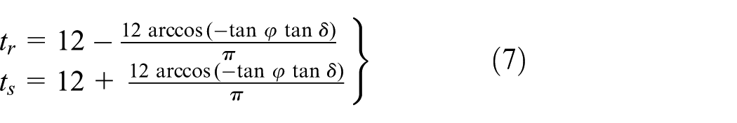

where tr and ts are the duration time of the sun on the horizontal surface of the track slab, t1 and t2 are the time calculated by the solar angle on the vertical surface of the track slab, and trv and tsv are the true sun moment on the vertical surface of the track slab.
Finite element analysis method of temperature field model based on ABAQUS
Finite element analysis is used to simulate the real physical system (geometry and load conditions) by means of mathematical approximation. 18 The real system of infinite unknowns can be approximated by a finite number of unknowns using simple and interacting elements. 19
The temperature field of
The

where T is the temperature at any point in the track slab; and x, y, and z are the coordinates of the width, height, and length of the track slab, respectively; and τ is the time.
According to the law of energy conservation and transformation, the heat conduction differential equation is as shown in equation (10), without considering the heat generation of the heat source in the concrete itself 21

where Ti is the temperature of the ith layer of the orbital structure, λi is the thermal conductivity of the ith layer (J/(m·s·K)), ρi is the density of the ith layer (kg/m3), and ci is the specific heat capacity of the ith layer (J/kg·k).
The steps for establishing a temperature field analysis model of the
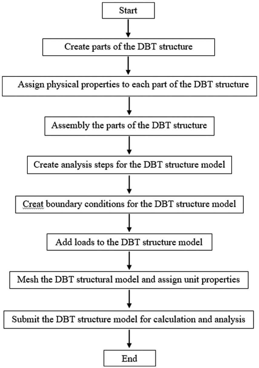
Steps for establishing the temperature field analysis model of the
1. Physical conditions
The
Physical parameters of

2. Boundary conditions
The boundary conditions mainly reflect a certain degree of interrelation between the object studied and the surrounding environment. In this article, boundary conditions are divided into surface boundary conditions of track structure, internal contact surface boundary conditions of track structure, and surface boundary conditions under the subgrade.
Surface boundary condition of track structure is that the convective heat transfer and the radiative heat transfer coexist on the surface of the track structure, which is a complex case of the third type of boundary conditions in heat transfer 23 and can be expressed in equation (11)

where
The internal contact surface boundary condition of track structure is that the contact surfaces of the sleeper, track slab, base plate, and subgrade are closely fitted in the absence of diseases such as separation, and all meet the fourth type of contact condition of heat transfer, that is, the temperature of the contact surfaces is equal, and the heat flux density of the contact surfaces is also equal.
The surface boundary condition under the subgrade is that the heat conduction between the lower surface of the substrate and the earth is neglected when establishing the temperature field model without considering the seasonal temperature change. The temperature and temperature gradients gradually decrease as the depth of the track structure increases. When the depth exceeds 20 cm, the temperature tends to be substantially stable and the fluctuation is small.
3. Loadings
Considering the actual operation of the DBT structure, the external loading conditions are divided into three types such as initial temperature field, external temperature loading, and solar radiation loading.
The initial conditions of the temperature field of the track structure are complicated, but under the same environmental conditions, after repeated loading for many times, the temperature field of the track structure tends to be stable. Reflected in the actual situation is the temperature field formed in the track structure when the weather is relatively stable for a long time. In this article, the results of repeated loading are selected to eliminate the influence of the initial temperature field in the calculation.
The external temperature loading is mainly the atmospheric temperature. The change of atmospheric temperature is affected by many factors, and the change is complicated. In this article, the hourly atmospheric temperature measurement value of the test site is directly selected as the loading data, which has high precision. 24
The solar radiation loading has a certain relationship with geographical latitude, atmospheric transparency, solar time angle, and solar incident angle. For different geographical factors, equation (3) is used to calculate the corresponding loading data.
4. Units and analysis steps
The temperature field analysis model belongs to pure thermal analysis. In this article, the DBT structure is modeled by three-dimensional solids. The sleeper, track bed board, base plate, and roadbed are all DC3D8 (an eight-node linear heat transfer brick) units. There are two types of steps, namely, the initial analysis step and the heat transfer analysis step.
Through the above steps and methods, the temperature field calculation model of the

Finite element model of
Finite element temperature field model verification of CRTS-I DBT structure
Model conditions
Experimental data were collected from 7 June 2014 through 13 July 2015 at the Qingrong intercity railway DBT in the Shandong Province for the determination of temperature load and boundary conditions. The solar radiation and atmospheric temperatures were collected during the period of highest temperatures in the year (14–21 July 2014) to obtain the most unfavorable values to serve as boundary conditions. The geographical latitude of 37.5°N was used to calculate the solar radiation. 25 The normal directions of the two sides of the track slab were taken from the angles 0° and −180° from the positive south direction to determine the sunshine time on the top of the track slab from 5:00 to 19:00. The sunshine time on one side of the track slab was from 5:00 to 19:00, and the other side remained in the shade all day. The average wind speed was assumed to be 3 m/s because of its coastal plain area location.
Model verification
Experimental points were arranged on the subgrade between the Taojiatong Tunnel and Wangjiazhuang Bridge at the Qingrong intercity railway. Data collection was carried out by Veriteq Spectrum’s automatic acquisition system, and the acquisition frequency was 1 time/h. The temperature sensor used a thermal resistance temperature sensor with a range of −200°C to 850°C and an accuracy of ±0.3°C. 26 In this article, the measuring point 5 in the middle of the vertical axis of the track slab, the measuring point 1 at the top of the edge of the track slab, the measuring point 2 in the middle of the edge of the track slab, and the measuring point 3 at the bottom of the edge of the track slab were selected for temperature verification, 27 as shown in Figure 4.

Track slab measurement point layout.
The temperature field model of a

Temperature distribution diagram of

Comparison diagram of experimental data and model data for each temperature measuring point: (a) temperature measuring point 1, (b) temperature measuring point 7, (c) temperature measuring point 3, and (d) temperature measuring point 5.
As shown in Figure 6, the experimental data at each measuring point were in agreement with the model data for the temperature cycle, vibration amplitude, and numerical value. 28
The next step in model validation was to adopt an improved Euclidean distance formula incorporating a balanced offset factor and the similarity of two time-series experimental data. The model data were then analyzed respectively. 29 The adopted formula is shown in equation (12)

where D(A, B) is the Euclidean distance, ai is the temperature time-series experimental data, bi is the temperature time-series model data point, m is the balance offset factor, and n is the total number of data points. The lower the Euclidean distance, the closer the two sets of time-series data. 30
The measuring points of average calculated Euclidean distances 1, 3, 5, and 7 were 0.2167°C, 0.1314°C, 0.1971°C, and 0.3597°C, respectively. Since all the distances were less than 0.5°C, the temperature field model of the developed
Time variation analysis of each temperature measuring point
The data collected from the weather during the experiment showed that the highest temperature and the highest temperature difference were on 20 July. Therefore, the track slab was divided into 29 parts from east to west; 30 nodes at the top of the slab and 30 nodes at the bottom of the slab were selected, as shown in Figure 5, to further explore the time-varying regularity of each node on 20 July, as shown in Figures 7 and 8.
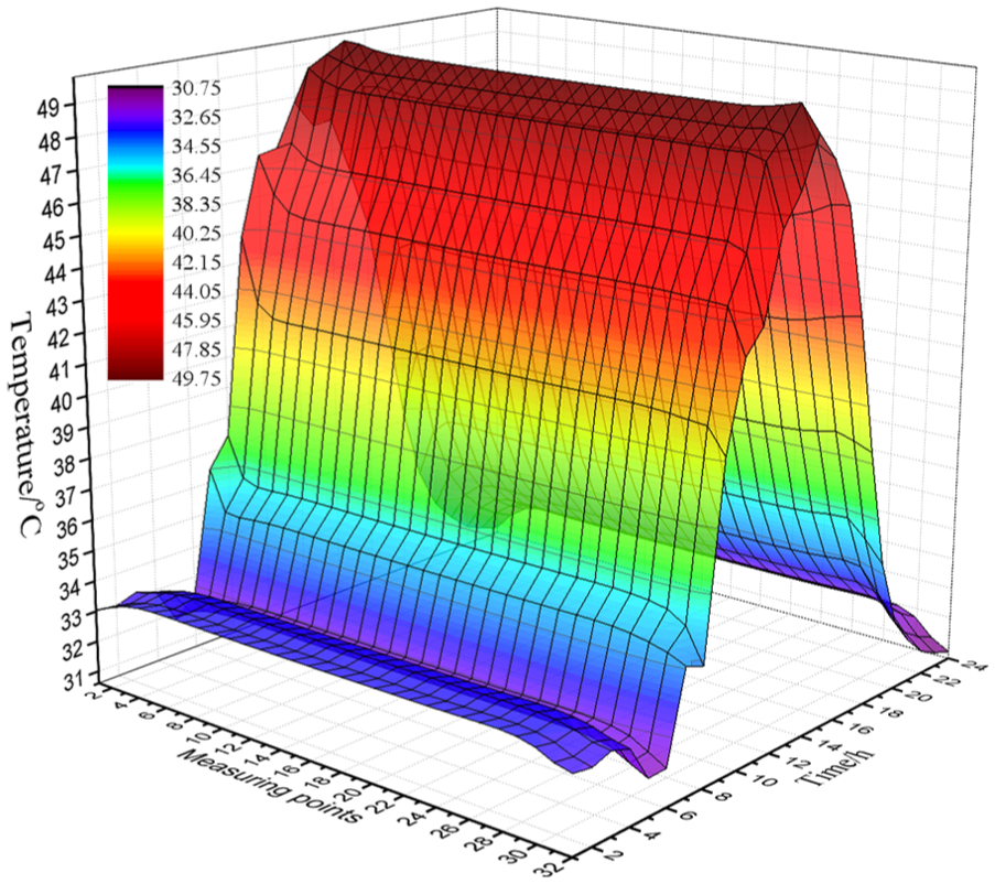
Temperature evolution with time at each node at the top of the track slab on 20 July.
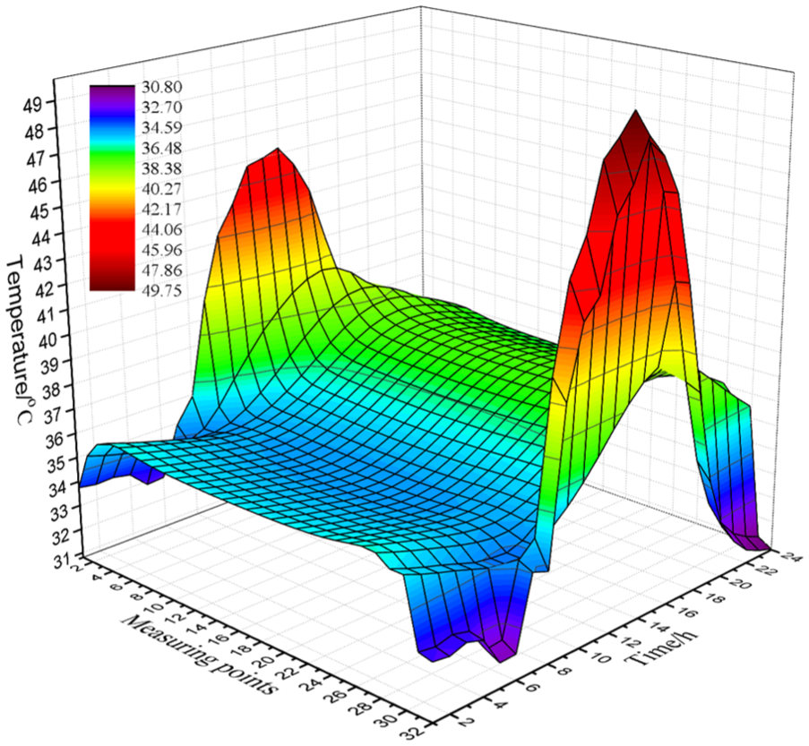
Temperature evolution with time at each node at the bottom of the track slab on 20 July.
The temperature curves on the top of the ballast bed nodes are mostly parabolic. The nodes at the bottom of the ballast bed and temperature changes of the nodes in the middle region are relatively gentle, whereas the temperature changes on other sides are relatively violent. Some specific features are presented in Table 2.
Ttime-varying features of the temperature of the track slab on 20 July 20.

As shown in Table 2, the temperature variation of nodes on both sides and middle of track slab is representative of, along with the changes of external environmental factors, such as solar radiation. Therefore, the variation of the temperature field of the track slab was further explored.
Influence of route direction on temperature field of CRTS-I DBT structure
To further explore the impact of the line direction on the temperature field of the track slab, 37.5°N (Qingdao, Shandong, China) was selected as the latitude for exploration, αn was divided into 24 parts from −180° to 180°, and the temperature field of 14–21 July was analyzed at every 15°. The temperature distribution in the track slab under the same latitude and different αn angles was obtained for the selected locations as shown in Figure 4.
Influence of route direction on horizontal temperature gradient of track slab
The moment is a characteristic used to describe the probability distribution of a random variable. The second-order origin moment refers to the variance of the random variable relative to the origin 31 and is used to measure the degree of deviation between the random variable and the origin; the larger the second-order origin moment, the greater the fluctuation of the data phase relative to the origin, and the smaller the second-order origin moment, the smaller the fluctuation of the data relative to the origin. The third-order origin moment refers to the skewness of the random variable relative to the origin and is mainly a measure describing the direction and extent of the skew of the statistical data relative to the origin. 32 Therefore, by calculating the moment, the distribution law and the state of the random variable can be obtained.
The temperature gradient origin was set to 0°C/m to explore the most unfavorable conditions of the horizontal temperature gradient of the track slab. The third-order moment of origin standard value was calculated to describe the direction and degree of skewness of the horizontal temperature gradient data distribution relative to the origin. 33 In addition, the second-order moment of origin standard value was used to describe the deviation of the horizontal temperature gradient relative to the origin. These are displayed in equations (13) and (14), and their calculated values are displayed in Figures 9 and 10

here, μ is the third-order moment of origin standard value, δ is the second-order moment of origin standard value, t is the modeled temperature data point, T0 is the temperature origin, and N is the number of data points.
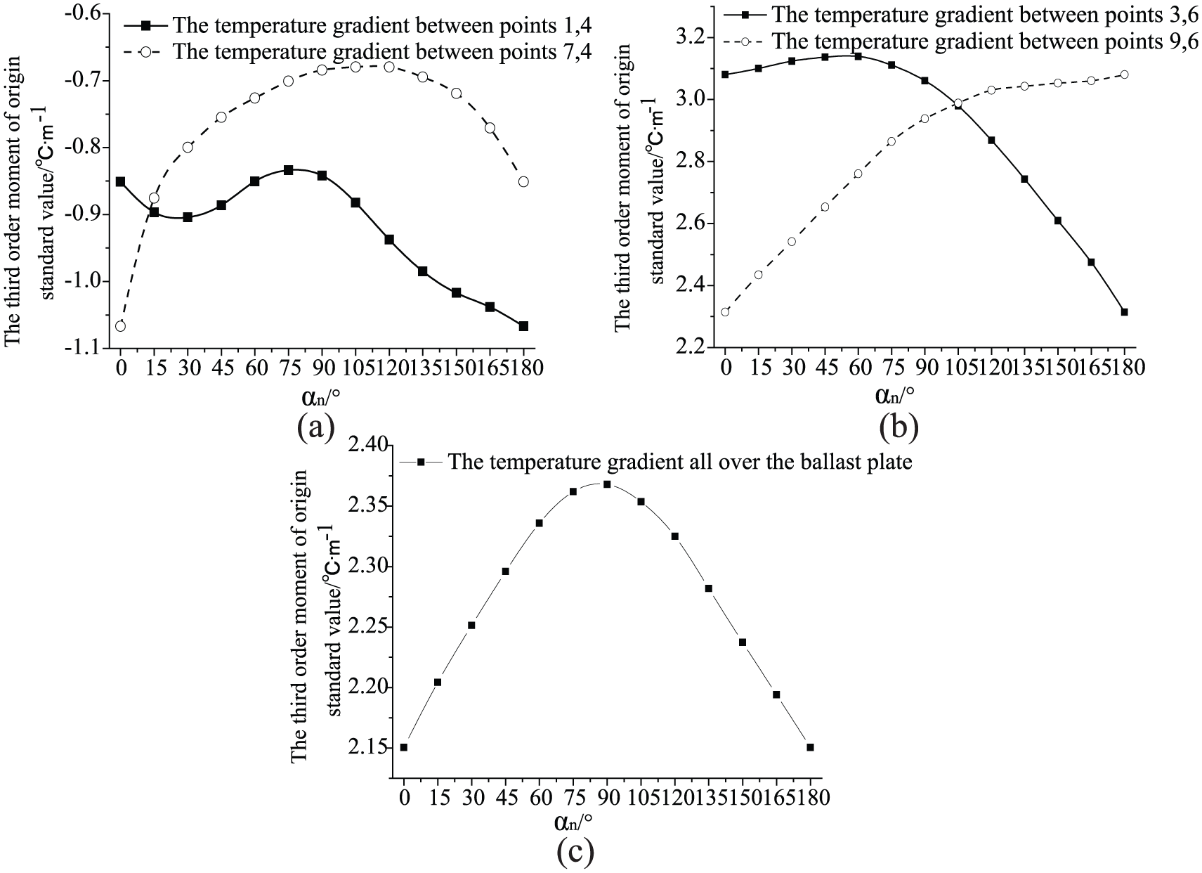
Third-order moment of origin standard value of the horizontal temperature gradient at the measuring points of the track slab at each αn angle: (a) top of the track slab, (b) bottom of the track slab, and (c) over the entire track slab.

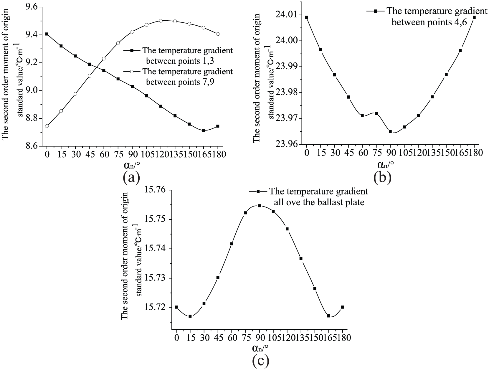
Second-order moment of origin standard value of the horizontal temperature gradient at the measuring points of the track slab at each αn angle: (a) top of the track slab, (b) bottom of the track slab, and (c) over the entire track slab.
As shown in Figure 9, the temperature gradient was influenced by changing the αn angle. The temperature gradient between measuring points 3 and 6 and between measuring points 9 and 6 was positive to the origin. Thus, the temperature on both sides of the bottom of the track slab was higher than that of the mid-plate. The temperature gradient between measuring points 1 and 4 and between measuring points 7 and 4 was negative to the origin, indicating that the temperature on both sides of the top of the track slab was lower than that of the mid-plate.
For αn = 180°, the largest value of the third-order moment of origin standard value between measuring points 1 and 4 was −1.070°C/m. For αn = 0°, the largest third-order moment of origin standard value between measuring points 7 and 4 was −1.071°C/m. For αn = 60°, the largest third-order moment of origin standard value between measuring points 3 and 6 was 3.137°C/m. For αn = 180°, the largest third-order moment of origin standard value between measuring points 9 and 6 was 3.082°C/m.
For αn = 90°, the largest third-order moment of origin standard value of the horizontal temperature gradient over the entire track slab was 2.374°C/m, indicating that the horizontal temperature gradient at this αn value had the largest skewness. When αn was equal to 0° or 180°, the smallest third-order moment of origin standard value of the horizontal temperature gradient over the entire track slab was 2.150°C/m.
As shown in Figure 10, for αn = 90°, the largest second-order moment of origin standard value between measuring points 1 and 4 was 1.007°C/m. For αn = 0°, the largest second-order moment of origin standard value between measuring points 7 and 4 was 1.001°C/m. For αn = 60°, the largest second-order moment of origin standard value between measuring points 3 and 6 was 3.092°C/m. For αn = 180°, the largest second-order moment of origin standard value between measuring points 9 and 6 was 3.031°C/m.
For αn = 90°, the largest second-order moment of origin standard value of the horizontal temperature gradient over the entire track slab was 2.189°C/m, indicating that the horizontal temperature gradient at this αn value had the largest deviation. When αn was equal to 0° or 180°, the smallest second-order moment of origin standard value of the horizontal temperature gradient over the entire track slab was 2.109°C/m.
In summary, the horizontal temperature gradient over the entire track slab was positive with respect to the origin at each αn angle. The horizontal temperature gradient over the entire track slab has the largest degree of skewness and the largest deviation from the origin when αn was equal to 90°. Therefore, the horizontal temperature gradient over the entire track slab was in the most unfavorable situation.
Influence of route direction on vertical temperature gradient of track slab
The skewness and standard deviation of the model were further explored to determine the effect of the line direction to the vertical temperature gradient on the track slab. The results are presented in Figures 11 and 12.

Third-order moment of origin standard value of the vertical temperature gradient at the measuring points of the track slab at each αn angle: (a) top of the track slab, (b) bottom of the track slab, and (c) over the entire track slab.
Second-order moment of origin standard value of the vertical temperature gradient at the measuring points of the track slab at each αn angle: (a) top of the track slab, (b) bottom of the track slab, and (c) over the entire track slab.
The temperature gradient between each measuring point was found to be positive to the origin, meaning that the temperature at the top of the track was higher than that of the bottom. As shown in Figure 11, for αn = 0°, the largest third-order moment of origin standard value between measuring points 1 and 3 was 9.494°C/m. For αn = 180°, the largest third-order moment of origin standard value between measuring points 7 and 9 was 9.492°C/m. When αn was equal to 0° or 180°, the largest third-order moment of origin standard value between measuring points 4 and 6 was 26.454°C/m.
When αn was equal to 90° or 180°, the largest third-order moment of origin standard value of the vertical temperature gradient over the entire track slab was 18.848°C/m, indicating that the vertical temperature gradient over the entire track slab had the largest deviation. For αn = 90°, the smallest third-order moment of origin standard value of the vertical temperature gradient all over the track slab was 18.736°C/m.
As shown in Figure 12, when αn was equal to 0°, the largest second-order moment of origin standard value between measuring points 1 and 3 was 9.413°C/m. For αn = 120°, the largest second-order moment of origin standard value between measuring points 7 and 9 was 9.479°C/m. When αn was equal to 0° or 180°, the largest second-order moment of origin standard value between measuring points 4 and 6 was 24.009°C/m. For αn = 90°, the largest second-order moment of origin standard value of the vertical temperature gradient all over the track slab was 15.754°C/m, indicating that the vertical temperature gradient over the entire track slab had the largest degree of dispersion. When αn was equal to 15° or 175°, the smallest second-order moment of origin standard value of the vertical temperature gradient all over the track slab was 15.717°C/m.
In summary, the vertical temperature gradient over the entire track slab was positive at each αn angle. The vertical temperature gradient has the largest degree of dispersion and smallest deviation at αn = 90°. Meanwhile, the vertical temperature gradient was greater and fluctuated more rapidly. Therefore, the vertical temperature gradient over the entire track slab was in the most unfavorable situation at αn = 90°.
Most unfavorable line direction determination based on temperature gradient
To determine the most unfavorable situation of the total temperature gradient of the track slab caused by the direction of the line, the third- and second-order moments of origin standard value were further explored, as shown in Figures 13 and 14.

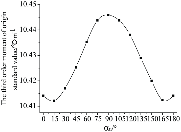
Third-order moment of origin standard value of the total temperature gradient of the track slab measuring points at each αn angle.
Second-order moment of origin standard value of the total temperature gradient in the measuring points of the track slab at each αn angle.
The total temperature gradient at each measuring point was found to be positive with respect to the origin; the temperatures at the top of the track slab were higher than the temperatures at the bottom, and the temperatures at the sides of the track slab were higher than the temperatures in the middle. As shown in Figure 13, for αn = 90°, the smallest third-order moment of origin standard value was 14.138°C/m. As αn gradually changed from 90° to 0° and from 90° to 180°, the third-order moment of origin standard value of the total temperature gradient gradually increased until reaching a maximum value of 14.220°C/m when αn was equal to 0° or 180°.
As shown in Figure 14, for αn = 90°, the largest second-order moment of origin standard value of the total temperature gradient was 10.446°C/m. As αn gradually changed from 90° to 0° and from 90° to 180°, the second-order moment of origin standard value of the total temperature gradient gradually decreased until reaching a minimum value of 10.412°C/m when αn was equal to 15° or 165°.
In summary, the total temperature gradient over the entire track slab was found to be positive at all αn angles. When αn was equal to 90°, the total temperature gradient had the largest degree of dispersion and smallest deviation. The total temperature gradient was greater and fluctuated more rapidly. Therefore, the total temperature gradient over the entire track slab was in the most unfavorable situation at αn = 90°.
Influence of geographical latitude on temperature field of CRTS-I DBT structure
The next step was to explore the influence of the change in geographical latitude on the temperature field of the track slab. The direction of the line was chosen such that αn = 90° and 43.77°N (Urumqi, Xinjiang, China), 37.5°N (Shandong, Shandong, China), 28.1°N (Changsha, Hunan, China), and 18.2°N (Sanya, Hainan, China) were selected to explore their geographical latitudes. A change in double sine function reflecting the law of temperature was observed during a sunny day 34 and was used to fit the temperature dynamics around these regions as shown in equation (15)

where E(T) is the average daily temperature; ΔT is the difference between the daily maximum temperature and the minimum temperature; τ is the time with 6:00 a.m. corresponding to 0; τ0 is the time constant, assumed to be 3 h; and ω is the frequency, where ω = 2π/24. The temperature data of all regions were obtained by the meteorological network. 35
Sunny day temperatures and solar radiation from July were used as model conditions to obtain the temperature field changes of the track slab under the same route directions and different geographical latitudes 36 to explore the temperature gradient variation.
Influence of geographical latitude on horizontal temperature gradient of track slab
The third- and second-order moments were explored to determine the most unfavorable situation of the horizontal temperature gradient of the track slab caused by varying geographical latitudes. Results are presented in Figures 15 and 16.

Third-order moment of origin standard value of the horizontal temperature gradient at the measuring points on the track slab at each geographical latitude.

Second-order moment of origin standard value of the horizontal temperature gradient at the measuring points of the track slab at each geographical latitude.
Of the two coastal areas, the skewness of the horizontal temperature gradient of the measuring points on the track slab in Sanya was found to be greater than that of Qingdao. Of the two inland areas, the skewness of the horizontal temperature gradient between the measuring points of the track slab was greater in Changsha than in Urumqi. In addition, the skewness of the horizontal temperature gradient of the measuring points on the track slab in Changsha was greater than in Sanya. Thus, the skewness of the positive temperature gradient in the coastal area was higher than that of the inland area and higher in the low-latitude area than in the high-latitude area.
Of the two coastal areas, the second-order moment of the horizontal temperature gradient between the measuring points of the track slab was greater in Qingdao than in Sanya. Of the two inland areas, the second-order moments in Urumqi were greater than that of Changsha. Furthermore, the degree of dispersion for the horizontal temperature gradient was greater in the inland and high-latitude areas than in the coastal and low-latitude areas.
In summary, the horizontal temperature gradient of the track slab was greater in the inland area of high latitude and incurred more rapid changes, making this the most unfavorable situation.
Influence of geographical latitude on vertical temperature gradient of track slab
The third- and second-order moments were then explored to determine the most unfavorable situation of the vertical temperature gradient of the track slab caused by varying geographical latitudes. Results are shown in Figures 17 and 18.

Third-order moment of origin standard value of the vertical temperature gradient at the measuring points of the track slab at each geographical latitude.

Second-order moment of origin standard value of the vertical temperature gradient at the measuring points of the track slab at each geographical latitude.
Of the two coastal areas, the third-order moment of the vertical temperature gradient between the measuring points of the track slab was greater in Sanya than in Qingdao. Of the two inland areas, the third-order moment of the vertical temperature gradient between the measuring points on the track slab was greater in Changsha than in Urumqi. In addition, the third-order moment of the vertical temperature gradient between the measuring points of the track slab was greater in Changsha than in Sanya. In this wise, the positive temperature gradient in the coastal area was higher than that of the inland area and higher in the low-latitude area than in the high-latitude area.
Of the two coastal areas, the second-order moment of the vertical temperature gradient at the measuring points on the track slab was greater in Qingdao than in Sanya. Of the two inland areas, the second-order moment of the vertical temperature gradient at the measuring points on the track slab was greater in Changsha than in Sanya. Thus, the degree of dispersion for the vertical temperature gradient in the inland and high-latitude areas was greater than that of the coastal and low-latitude areas.
In summary, the vertical temperature gradient of the track slab was greater in the inland area of high latitude and incurred more rapid changes, making this the most unfavorable situation.
Most unfavorable geographical latitude determination based on temperature gradient
As demonstrated in sections “Influence of geographical latitude on horizontal temperature gradient of track slab” and “Influence of geographical latitude on vertical temperature gradient of track slab,” the horizontal and vertical temperature fields of the track slab in the inland and high-latitude areas were more unfavorable than the coastal and low-latitude regions. The third- and second-order moments were further explored to determine the most unfavorable situation of the total temperature gradient of the track slab caused by varying geographical latitudes. The results are shown in Figures 19 and 20.
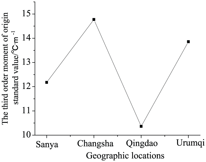
Third-order moment of origin standard value of the total temperature gradient at the measuring points of the track slab in each area.

Second-order moment of origin standard value of the total temperature gradient at the measuring points of the track slab in each area.
Of the two coastal areas, the third-order moment of the total temperature gradient at the measuring points on the track slab was greater in Sanya than in Qingdao. Of the two inland areas, the third-order moment of the total temperature gradient between the measuring points on the track slab was greater in Changsha than in Urumqi. In addition, the third-order moment of the total temperature gradient at the measuring points on the track slab was greater in Changsha than in Sanya. The positive temperature gradient was greater in the coastal and low-latitude areas than in the inland and high-latitude areas.
Of the two coastal areas, the second-order moment of the total temperature gradient between the measuring points on the track slab was greater in Qingdao than in Sanya. Of the two inland areas, the second-order moment of the total temperature gradient at the measuring points on the track slab was greater in Urumqi than in Changsha. In addition, the second-order moment of the total temperature gradient at the measuring points on the track slab was greater in Changsha than in Sanya. Thus, the degree of dispersion for the total temperature gradient was greater in the inland and high-latitude areas than in the coastal and low-latitude areas.
In summary, the skewness was greater in the coastal and high-latitude areas than in the inland and low-latitude areas. The degree of dispersion was greater in the inland and high-latitude areas than in the coastal and low-latitude areas. Therefore, in inland areas of high latitudes, the total temperature gradient of a track slab is greater and faces more rapid changes demonstrating the most unfavorable situation.
Conclusion
From this study, the following conclusions can be drawn:
A temperature field analysis model of a CRTS-I DBT structure, based on solar radiation and boundary-surface heat transfer theory, was established and calculated using ABAQUS finite element software. The Euclidean distance between model data and experimental data was less than 0.5°C. Therefore, the model has the higher adaptability to the actual working conditions.
The second- and third-order moments of the horizontal temperature gradient over the entire track slab were greater when the angle between the normal and the south directions of the track slab was equal to 90° at 2.37 and 2.19°C/m, respectively. The greater values of the second- and third-order moments of the vertical temperature gradient over the entire track slab were 15.75 and 18.74°C/m, respectively. At this point, the horizontal and vertical temperature gradients of the track slab were in the most unfavorable conditions.
The second- and third-order moments of the total temperature gradient over the entire track slab were greater when the angle between the normal and the south directions of the track slab was equal to 90° at 10.45 and 14.13°C/m, respectively. Thus, at this angle, the temperature gradient was greater and experienced more rapid changes. Therefore, the total temperature gradients of the track slab were in the most unfavorable situation.
The horizontal and vertical temperature gradients in the high-latitude and coastal areas were found to be more detrimental than that in the low-latitude and inland areas for the DBT structure with the line direction αn of 90°.
The most unfavorable situation for the total temperature gradient of the track slab was found in the inland area of high latitude, where the total temperature gradient was greater and experienced more rapid changes.
Footnotes
Handling Editor: Luca Furgani
Declaration of conflicting interests
The author(s) declared no potential conflicts of interest with respect to the research, authorship, and/or publication of this article.
Funding
The author(s) disclosed receipt of the following financial support for the research, authorship, and/or publication of this article: This work was supported by the Graduate Innovation Project of Central South University (grant no. 2018zzts649), the Major Program of National Natural Science Foundation of China (grant no. 11790283), the High-Speed Railway Joint Fund of National Natural Science Foundation of China (grant no. U1734208), and the Science and Technology Foundation of China Railway 14th Bureau Corporation Limited (grant no. 20160016).