Sage Journals: Discover world-class research

Abstract

In order to study the change rules of interior acoustic field with the development of cavitation, this article presented a method that through comparing the experiment results with numerical simulation results in cavitation bubbles’ distribution images under different cavitation coefficients to optimize the accuracy of acoustic field simulation using computational fluid dynamics combined with the Lighthill acoustic analogy. First, a closed visual testing system was established based on pump product test system and high-speed photography. Second, the cavitation performance under the rated operating condition was calculated using different cavitation models, in order to obtain both pump cavitation performance curve and distribution of cavitation bubbles. Next, based on the external characteristics experiment and high-speed photography experiment, the appropriate cavitation model for unsteady numerical calculation was selected. On the basis of vapor volume fraction distribution and the cavitation performance curve, four different typical points representing different cavitation coefficients were selected for further analyses. The direct boundary element method was used to calculate the variation characteristics of cavitation-induced noise at different cavitation coefficients. Finally, the peak-to-peak value of pressure fluctuation coefficient is defined as Д, and the pressure pulsating frequency domain signals were analyzed to further study the influence of pressure pulsation on acoustic field. The results show that the effect of pressure pulsation on noise is mainly focused on the discrete eigenvalues, and as for the broadband noise, the influence is not obvious. With the development of cavitation, axial passing frequency, 10- to 100-Hz frequency band, and 1000- to 3000-Hz frequency band show an increasing trend, while blade passing frequency and its harmonic frequencies show a decreasing trend. At the onset of cavitation, 1000- to 3000-Hz frequency band has the highest sensitivity for cavitation detection.

Keywords

Centrifugal pump cavitation noise pressure fluctuation high-speed photography numerical simulation

Introduction

As an important energy conversion equipment and fluid transportation equipment, centrifugal pumps are widely used in various fields, such as submarines, aerospace, and other advanced technology fields.^1–3 Cavitation, which has been restricted to the development of the pump industry, presents unwanted consequence. Cavitation results in the destruction of the material surface, causing unreliability of pump operation, while vibration and noise affect the operational stability. Hence, cavitation not only limits the high-efficient operating range of centrifugal pumps, but also plays a restrictive role in the development direction of small-size and high-speed of centrifugal pumps.^4,5

According to cavitation characteristics, there are some judgment methods to detect cavitation. For example, the cavities collapsing lose to a solid component that sprayed specific paint and if the amplitude of the resulting pressure pulse is larger than the limit of the paint allowable strength, several micrometers called “pit” will be formed on the surface; the method called determination of coating erosion is a original method for cavitation judgment. The difficulty of this method is choosing the proper adhesivity and sensitivity of paint. Second, determination of the net positive suction head (NPSH) is the most popular engineering method. According to standards, the NPSH value is determined by a 3% drop in total head, which represents the character value on behalf of complete development of cavitation. This method needs a special test stand prescribed by the standards and a set of measurement results to determine the required value of NPSH at different flow rates. What is more, according to the relationship between the efficiency, flow rate, torque, and the critical cavitation coefficient to judge the degree of cavitation called energy method, there is another one being used in detection of cavitation in model machine. Unfortunately, the pump efficiency does not decrease immediately when the cavitation occurs. In addition, high-speed photography and stroboscopy are common methods in detecting cavitation, but all these methods have their own disadvantages.

A rarely used engineering method based on sound pressure and pressure pulsation measurement is simple and logical. It can be clearly “heard” by noise transducer when cavitation appears. So, the appearance and development of cavitation can be monitored using acoustic signal. Hence, cavitation within pumps has been the subject of extensive research up to now, as demonstrated by the works from the following scholars. Acoustic emission technology was used by Alfayez and colleagues,^6,7 to establish the criterion of cavitation initiation, which can be more accurate to monitor the initial cavitation. But this method has some defects in the detection of non-optimum conditions. B Zeqiri et al.⁸ measured the vibration and noise characteristics of the centrifugal pump by means of an acceleration sensor and a microphone. It was found that there was a positive correlation between cavitation and vibration noise, and the vibration noise signal corresponds to the degree of cavitation damage to some extent. Cudina et al.^9–11 found that there is a discrete frequency eigenvalue in the noise spectrum corresponding to the process of internal cavitation development of the pump, which, as a basis for cavitation detection, is more accurate compared with industrial traditional methods. Chini et al.¹² measured the vibration signal of the centrifugal pump in cavitation and non-cavitation conditions and proposed a method for online instantaneity monitoring of cavitation in centrifugal pump. Bajic¹³ carried out a multidimensional monitoring research to the cavitation of the turbine and realized accurately recognizing the position of the cavitation. Based on this, cavitation characteristic development trend can be predicted. Using wavelet transform (WT), Qi and Shen¹⁴ did some research on cavitation noise signal to study the variation of the wavelet coefficients with time and frequency and the variation of the cavitation noise spectrum with time. Z Pu et al.¹⁵ studied the cavitation of the turbine and proposed a method of detecting the cavitation of the turbine based on the wavelet singularity theory to detect the cavitation of the turbine and the cavitation transformation. A lot of research works have been done on cavitation-induced noise by Leighton,¹⁶ Fanelli,¹⁷ and Li¹⁸ and proposed some corresponding numerical simulation method. The method for obtaining cavitation noise of centrifugal pumps is mainly through experimental way. With the development of acoustic field calculating method, there are three means for noise calculation.^19–21 (1) The direct calculating method—the basic idea is to solve the noise directly by hydrodynamics and it can only be solved by detached eddy simulation (DES) and large eddy simulation (LES) methods. (2) Semi-empirical model method—the basic idea is to solve the flow field information based on Reynolds average equation first and acoustic field is then solved based on semi-empirical formula. (3) Method based on acoustic analog equation—the basic idea is to solve the flow field information by computational fluid dynamics (CFD) method and then the acoustic field is calculated based on acoustic analogy equation. Far-field noise has a higher degree of confidence than the accuracy of calculating near-field noise. Fluid-acoustic coupling method belongs to the third one. Until now, only a few references use the fluid-acoustic coupling method to calculate the cavitation noise in the centrifugal pump. Z Yunlong and Yuanzheng²² calculated the flow field and acoustic field information using the method of fluid-acoustic method coupling LES. The whole cavitation progress was subdivided into three stages. The noise spectrum had big differences in different cavitation stages. Based on this, they considered that the degree of cavitation development can be reflected in the spectrum of hydrodynamic noise. There is a clear characteristic of the noise spectrum trend especially in the vicinity of NPSH_c (critical net positive suction head). W Yong et al.²³ employed Zwart cavitation model to simulate the cavitation flow field, which is verified to be more suitable for ultralow-speed centrifugal pump. By combining boundary element method (BEM), the acoustic filed was transformed through fluid field information. By dividing the entire cavitation process into four different stages, the variation regularities of cavitation noise signals at different stages are studied. Since the essence of the change of the acoustic field calculated by the flow-acoustic coupling method is caused by the change of the pressure pulsation on the surface of the sound source, the above reference works lack the exploration of its essence. Therefore, this article mainly focuses on the character changing laws of centrifugal pump by experiment investigation combining with numerical simulation to research the pressure pulsation and interior noise during the development of cavitation. The experimental investigation is to select the appropriate cavitation model to make the calculation more accurate.

Experimental test system

Experimental device consists of cavitation cylinder, surge tank, inlet and outlet pipes, valves, vacuum pump, motor, turbine flow meter, pressure transmitter, and other components (see Figure 1).

Figure 1.

Diagram of cavitation experimental system of centrifugal pump.

Experimental subject

In order to observe the cavitation bubble distribution in the inlet of impeller of the centrifugal pump, the relationship between the distribution of bubbles and cavitation-induced noise characteristics of centrifugal pump is lucubrated. The fully transparent pump was built by plexiglass, and the high-speed camera was used to synchronously capture the distribution of bubbles. The model pump is single-stage single-suction centrifugal pump, and the impeller type is closed. The inner circle with outer square structure is designed to reduce the refraction of light (see Figure 2).

Figure 2.

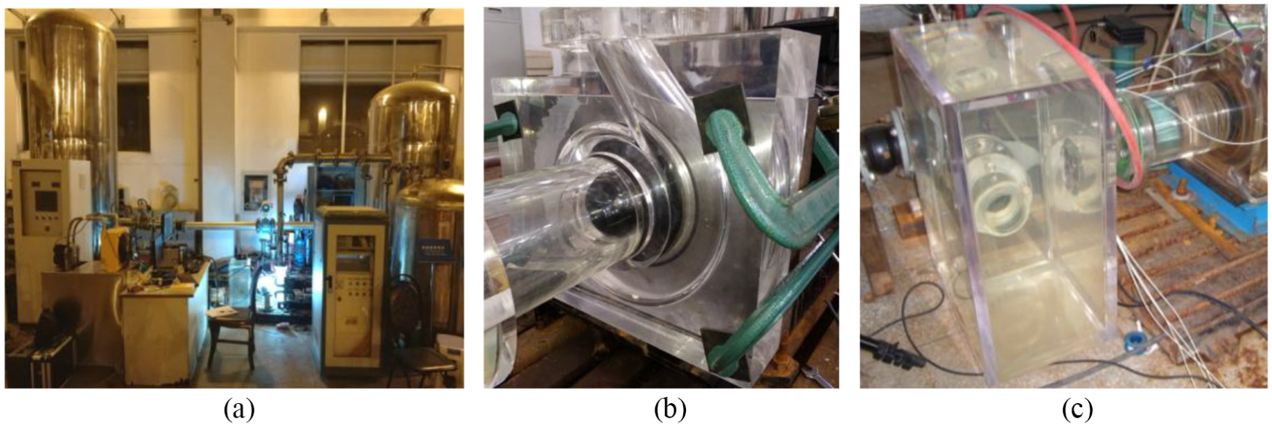
Picture of each test device: (a) test bench, (b) model pump, and (c) plexiglass tank.

Data collection system

The closed-type experimental system includes experimental device, pump performance parameter acquisition system, and centrifugal pump interior image acquisition system. In order to measure the cavitation pattern directly, a sealed water tank was placed at the inlet of the pump, which was placed on the side of the tank so as to place a high-speed camera. Taking into account that the performance of pump cannot be affected by the tank, the volume of the tank is designed to 0.1 m³, playing stabilizing flow role in the inlet of the pump.

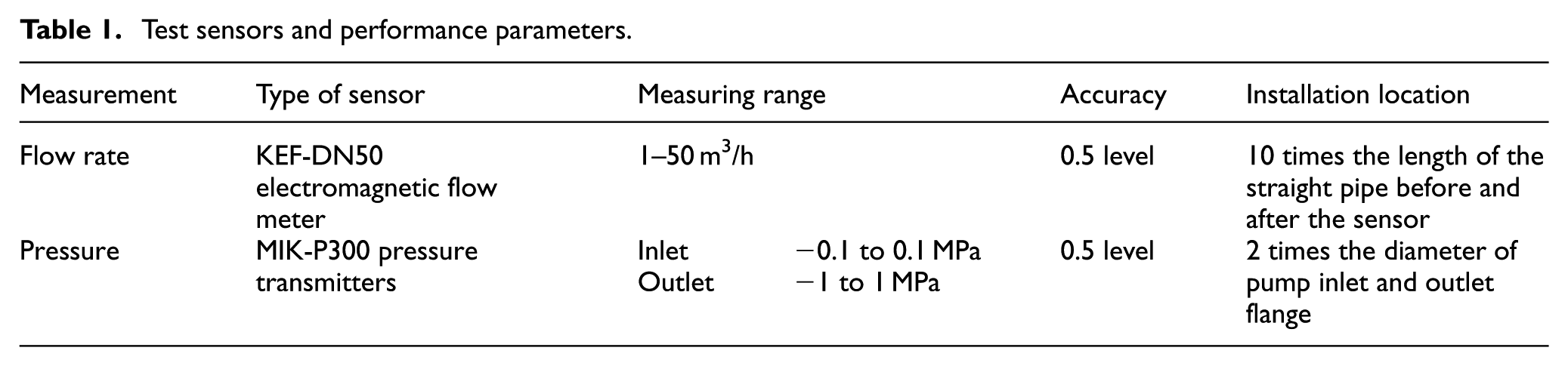
The pump parameter measuring instrument is used to collecting inlet and outlet pressure, flow rate, rotating speed, motor voltage, current, and power. The sensor details for measuring flow and pressure are shown in Table 1.

Table 1.

Test sensors and performance parameters.

Measurement	Type of sensor	Measuring range		Accuracy	Installation location
Flow rate	KEF-DN50 electromagnetic flow meter	1–50 m³/h		0.5 level	10 times the length of the straight pipe before and after the sensor
Pressure	MIK-P300 pressure transmitters	Inlet	−0.1 to 0.1 MPa	0.5 level	2 times the diameter of pump inlet and outlet flange
Pressure	MIK-P300 pressure transmitters	Outlet	−1 to 1 MPa	0.5 level	2 times the diameter of pump inlet and outlet flange

Besides, the high-speed camera, Y-series 4 L, manufactured by IDT, with the maximum resolution 1024 × 1024 and the full-resolution maximum shooting speed 4000 frames/s, was used. LED (light-emitting diode) light was passed from the side wall into the volute, and two halogen lamps were placed on both sides of the inlet tube.

Numerical calculation

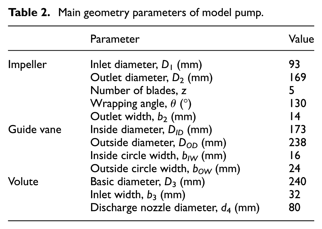
The main design parameters of this pump are as follows: Q_d (design flow rate) = 32.8 m³/h, H (head) = 8.1 m, n (rotating speed) = 1450 r/min, n_s (Chinese units: n_s = 3.6 nQ1/2/H^3/4) = 105. The other geometry parameters of the model pump are shown in Table 2.

Table 2.

Main geometry parameters of model pump.

	Parameter	Value
Impeller	Inlet diameter, D₁ (mm)	93
	Outlet diameter, D₂ (mm)	169
	Number of blades, z	5
	Wrapping angle, θ (°)	130
	Outlet width, b₂ (mm)	14
Guide vane	Inside diameter, D_ID (mm)	173
	Outside diameter, D_OD (mm)	238
	Inside circle width, b_IW (mm)	16
	Outside circle width, b_OW (mm)	24
Volute	Basic diameter, D₃ (mm)	240
	Inlet width, b₃ (mm)	32
	Discharge nozzle diameter, d₄ (mm)	80

Based on ANSYS ICEM CFD software, the calculation area of the model pump is divided into meshes; after checking whether the number of meshes is independent with the performance of calculation or not, it is generally recognized that if correlation of head is less than 1% with mesh number, there is no effect on the calculation results (see Table 3). Compared with five head prediction values of different numbers of meshes, the scheme 4, the meshing number of which is 1187634, is chosen through overall consideration. The mesh quality equals to 0.38, which satisfied the requirements of calculation (see Figure 3).

Table 3.

Inspection of grid independence.

Scheme	Impeller	Guide vane	Volute	Inlet and outlet pipes	Total grids	Head (m)
1	2.0 × 10⁵	1.8 × 10⁵	2.5 × 10⁵	1.2 × 10⁵	0.75 × 10⁶	8.61
2	2.7 × 10⁵	2.1 × 10⁵	2.8 × 10⁵	1.5 × 10⁵	0.91 × 10⁶	8.39
3	3.0 × 10⁵	2.4 × 10⁵	3.5 × 10⁵	1.5 × 10⁵	1.04 × 10⁶	8.24
4	3.4 × 10⁵	2.7 × 10⁵	4.2 × 10⁵	1.5 × 10⁵	1.18 × 10⁶	8.18
5	4.1 × 10⁵	3.5 × 10⁵	4.9 × 10⁵	2.2 × 10⁵	1.47 × 10⁶	8.19

Figure 3.

Grids of model pump.

Determination of turbulence and cavitation model

The internal flow of centrifugal pump is a complex three-dimensional (3D) turbulence, in which the flow parameters are random with temporal and spatial irregularities. There are a myriad of vortexes present with different size and shape, which vary with geometric space of flow field. Large-scale vortex depends on boundary conditions, forming and existing for a long time, while small vortex is random disorder. The SST (shear stress transport) turbulence model is usually used for low specific speed (≤80) centrifugal pumps; the standard k–ε turbulence model is usually used for medium to high specific speed (80–300) centrifugal pumps.²⁴ Based on this, we choose standard k–ε turbulence model to simulate.

As for cavitation flow, the basic equations are not closed because the number of unknown parameters (u, P, ρ) is more than the number of equations. So, the expression of relationship should be built about density of vapor–liquid mixing mediator with other physical parameters, that is, cavitation model. On the basis of the empirical formula, the dimensional factors affecting the cavitation are analyzed by Kunz et al.,²⁵ and the transport equation of the vapor volume fraction is established. The equation contains two source items: generating and condensing items of the steam. Based on Rayleigh–Plesset equation, Zwart et al.²⁶ cavitation model was established by solving the total mass transfer rate of the expression through the unit volume vacancy number and a single-bubble mass transfer rate.

The bubble distribution at the different cavitation numbers, predicted by the two cavitation models and pictured by high-speed photography, is shown in Figure 4.

Figure 4.

Cavitation bubble distribution of impeller at different cavitation coefficients: (a) σ = 0.549, (b) σ = 0.414, (c) σ = 0.310, and (d) σ = 0.215.

Define σ as the cavitation coefficient

σ = \frac{P_{i n} - P_{v}}{\frac{1}{2} ρ_{l} u_{2}^{2}}

(1)

where P_in is the inlet pressure of the impeller, P_v is the saturated vapor pressure, ρ_l is the medium density, and u₂ is the peripheral speed of impeller outlet.

From the test results, the blade inlet side of the suction surface begins to have small bubbles (initial cavitation as shown in Figure 4(a)) when σ = 0.549. The bubbles are attached to the blades all the time and cannot be separated from the blades due to the centrifugal force. So, the cavitation stage in centrifugal pump at this time is called attached cavitation. When σ = 0.414, it can be clearly observed that a large number of bubbles have been generated in the blade inlet side, which are generally in the form of sheet (sheet cavitation as shown in Figure 4(b)). The area and the thickness of the sheet of bubbles increase when the cavitation coefficient decreases. With the increase in the area and the thickness of the sheet cavitation, the plugging effect of bubbles on the flow channel is more obvious, which seriously affected the pump performance.

In the numerical calculation of cavitation, the bubble morphology mainly depends on the cavitation model. The final form of Zwart cavitation model, which is based on the formula of phase change rate introduced by the continuity equations of vapor and liquid, is obtained by modifying the phase change rate based on the generation and collapse of bubbles. The Kunz cavitation model has considered the generation and collapse of bubbles as two processes and obtains the expression of mass transfer rate in different ways. In addition, since the characteristic length and the free-flow velocity are related to the Reynolds number, Kunz cavitation model is more suitable for complex internal turbulent flow in the centrifugal pump. Comparing the experimental and simulated results, we can find that there are no cavitation bubbles simulated by Zwart cavitation model, while a small amount of bubbles can be effectively captured and simulated by Kunz model. So, the Kunz cavitation model is more accurate at the beginning of cavitation. When σ = 0.414 and σ = 0.310, the distribution of sheet cavitation on the blade surfaces is symmetrical. But there are no cavitations to generate at some blades simulated by Zwart cavitation model. So, the results simulated by Kunz cavitation model are more consistent with the actual situation. Thus, the Kunz cavitation model is chosen for unsteady numerical simulation.

The Kunz cavitation model is as follows

R_{e} = \frac{C_{d e s t} ρ_{ν} (1 - α_{ν}) MAX (P_{ν} - P, 0)}{\frac{1}{2} ρ_{l} U_{\infty}^{2} t_{\infty}}

(2)

R_{c} = \frac{C_{p r o d} ρ_{ν} α_{ν} {(1 - α_{ν})}^{2}}{t_{\infty}}

(3)

where U_∞ is the free-flow speed, L is the feature length, t_∞= L/U_∞ is the feature time scale, C_dest = 9 × 10⁵, C_prod = 3 × 10⁴, and p_v = 3574 Pa.

Selection of different cavitation coefficients

Based on the cavitation performance curve (see Figure 5) and the vapor volume fraction distribution (see Figure 6), four different points at the cavitation curve are chosen for further analyses.

Figure 5.

Cavitation performance curve.

Figure 6.

Vapor volume fraction distribution: (a) P1 (σ = 1.07), (b) P2 (σ = 0.44), (c) P3 (σ = 0.37), (d) P4 (σ = 0.24), (e) P1 (σ = 1.07), (f) P2 (σ = 0.44), (g) P3 (σ = 0.37), and (h) P4 (σ = 0.24).

The vapor volume fraction distributions at span = 0.5 (span is defined as the dimensionless distance from the shroud to the hub) along with the development of cavitation at different cavitation coefficients are shown in Figure 6. In order to intuitively explain the state and location of the cavitation bubbles in the impeller, the 3D graphic models are shown next. The blue zone represents low-pressure area, where the bubbles begin to generate, while the red zone represents high-pressure area, where the bubbles begin to collapse.

P1 (σ = 1.07) is located at the horizontal stage of cavitation performance curve and there is no vapor volume distribution in the suction side of blades from Figure 6(a). The cavitation performance has not been affected at P2 (σ = 0.44) position, while a small amount of bubbles begin to appear suction surface of blades. The hydraulic performance of pump has been influenced at P3 (σ = 0.37), the decreasing amplitude of head is about 3%, and the length of cavities along the blade suction surface side is about 1/3–1/2. At P4 (σ = 0.24) position, the flow channel of the impeller is occupied by a large number of bubbles, the bubble traces extend to the pressure side of the blade inlet, and the length of the bubble along the suction side of blades is more than 1/2 of the blade suction side. At this point, the performance of pump has been seriously affected.

In addition, as it can be seen from Figure 6, it is asymmetric for the distribution of cavities inside the impeller channel because the spiral case destroys the axial symmetry of the centrifugal pump and the impeller, and guide vane coupling effect makes the impeller blade surface pressure distribution asymmetrical.

Simulation of pressure and inner field noise by unsteady numerical calculation

The k–ε turbulence model is applied in the unsteady-state analysis and the average residual convergence criterion is set to 10⁻⁴. At the inlet of the computational domain, the mass flow rate is specified, and at the outlet boundary surface, the static pressure is set to zero. All walls of the flow domain are modeled using a non-slip boundary condition with 10-µm roughness. The flow field of the steady calculation is used as the initial condition for the unsteady simulation. In unsteady calculation, the time step is set to ΔT = 0.0000565 s corresponding to 360 time steps per impeller revolution. When flow field shows obvious periodicity and reaches stable state and extracts the last eight rotation periods as noise calculation excitation source. The pressure pulsation monitoring points are set every 10° along with impeller and guide vane circumference and set every 45° along with the volute circumference (see Figure 7).

Figure 7.

The pressure pulsation monitoring points’ setting in the pump.

For the interior field noise calculation, Lighthill sound analogy theory²⁰ is the basis of calculating and researching noise generated from rotating machinery; acoustic analogy equation can be derived from the conservation of fluid mass and momentum conservation

\frac{1}{c_{0}^{2}} \frac{\partial^{2} p^{'}}{\partial t^{2}} - \frac{\partial^{2} p^{'}}{\partial x_{i}^{2}} = \frac{\partial^{2}}{\partial x_{i} \partial x_{j}} (ρ v_{i} v_{j} - σ_{i j}) - \frac{\partial f_{i}}{\partial x_{i}} + \frac{\partial^{2}}{\partial t^{2}} (\frac{p^{'}}{c_{0}^{2}} - ρ^{'})

(4)

The flow rate in common centrifugal pump is less than Mach 0.35, so a special form of Lighthill equation called FW-H equation can be used for the acoustic solution of centrifugal pump

\begin{array}{l} \frac{\partial^{2} ρ^{'}}{\partial t^{2}} - c_{0}^{2} \nabla^{2} ρ^{'} = \frac{\partial^{2} T_{i j}}{\partial x_{i} \partial x_{j}} - \frac{\partial}{\partial x_{i}} [(p^{'} δ_{i j}) \frac{\partial f}{\partial x_{j}} δ (f)] \\ + \frac{\partial}{\partial t} [ρ_{0} u_{i} \frac{\partial f}{\partial x_{i}} δ (f)] \end{array}

(5)

where f is the control of the boundary function, and p represents the change of pressure that fluid is subjected to. The sound source information needed for the calculation of the field noise in the centrifugal pump is extracted directly from the unsteady fluid calculation results. The whole calculation process is implemented on the LMS Virtual.Lab platform. The fast Fourier transform (FFT) is used in noise calculation process to transform time–domain pulsation into frequency–domain pulsation. The data information is transferred to the acoustic grid by mapping. Acceleration is set to be the boundary condition and the inlet and outlet panels are defined as the sound absorption properties, while the other surfaces are total reflection. The acoustic impedance is set to 1.5 × 10⁶ kg m⁻² s⁻¹, the speed of sound in water is set to 1500 m/s, and the reference sound pressure in water is 1 × 10⁻⁶ Pa.

Calculation results and analysis

The change of the noise in different cavitation coefficients

The position of the field points are placed in eight times the diameter of the pump inlet and outlet pipe to ensure that the far field noise is measured. The human ear is not sensitive to low-frequency sound but not sensitive to high-frequency sound. “A” sound level is equivalent to human ear for 40-phon pure tone response, and the sound pressure–level curve is processed with A-weighting.

By comparing the sound pressure level (SPL) spectrum curve at different cavitation coefficients (Figure 8), we can find that the spectra show a significant frequency characteristic of blade passing frequency (BPF) and its harmonic frequencies, especially at P1 and P2. The BPF appears at the fifth peak value in the spectrum, which corresponds to the five blades of impeller. The SPL spectrum of the monitoring points at different locations of inlet and outlet has some slight differences at the same cavitation coefficient. The SPL gradually decreases with the increase in the frequency. When the frequency of the spectrum curve is larger than 300 Hz, the SPL of broadband begins to show a decreasing trend, which suggests that the attenuation of high-frequency energy is more rapid than low-frequency energy. And with the decrease in σ, the width of spectrum is gradually reduced and the high-frequency SPL is gradually increased and causes the eigenvalues to be suppressed in the broadband frequencies.

Figure 8.

The SPL spectrum curve monitored by inlet and outlet monitoring points at different cavitation coefficients: (a) SPL spectrum at P1 (σ = 1.07) (outlet monitoring point: left, inlet monitoring point: right); (b) SPL spectrum at P2 (σ = 0.44) (outlet monitoring point: left, inlet monitoring point: right); (c) SPL spectrum at P3 (σ = 0.37) (outlet monitoring point: left, inlet monitoring point: right); and (d) SPL spectrum at P4 (σ = 0.24) (outlet monitoring point: left, inlet monitoring point: right).

From Figure 8(a), there are discrete eigenvalues below BPF (120.8 Hz) in SPL spectrum, which maintains at about 140 dB. And the SPL at BPF reaches the highest value of the whole spectrum, which indicates that the main component of the exterior acoustic is still caused by the rotor–stator interaction between the rotating blade and the stationary volute tongue, which causes the discrete noise induced by the pressure fluctuation at P1. During 120.8- to 300-Hz frequency band, eigenvalues are basically reflected in the multiple harmonic frequencies of axial frequency. When frequency increases from 300- to 1000-Hz frequency band, the SPL drops from 150 to 130 dB, which indicates that the energy is mainly concentrated in the low-frequency band below 300 Hz. In the high-frequency band above 1000 Hz, the SPL shows a trend of fluctuation and drops rapidly below 2500 Hz frequency band.

From Figure 8(b), it can be seen that there is no significant change in the spectral curve compared with Figure 8(a). The SPL at BPF and its harmonic frequencies decrease slightly at P2 compared with P1; the same rule reflected in high-frequency band as well because pressure pulsation generated by the cavitation bubble movement and rupture has influence on the SPL. But a small amount of bubbles are not sufficient to cause changes in the physical properties such as fluid medium density, and the change of the flow field is neglectable. So, the change of SPL signal is small at this situation.

From Figure 8(c), it can be seen that the width of spectrum decreases significantly. And the discrete eigenvalues below BPF (120.8 Hz) increase, while it is no longer the number of eigenvalues corresponding to the number of blades of impeller. The SPL at BPF still decreases compared with the first two cavitation coefficients. The decrease in spectral width is caused by different reasons. First, the migration and collapse of a large number of cavitation bubble groups can increase the SPL of the middle- and high-frequency bands, and the cavitation noise has an obvious broadband characteristic, which causes the SPL of entire broadband to rise above 300 Hz. In addition, the energy of the eigenvalue components is gradually reduced at the frequency band above 300 Hz. So, the eigenvalues are gradually submerged in the wideband, causing the decrease in spectral width. Moreover, a large number of cavitation bubbles present at the inlet of impeller, a part of acoustic energy can be absorbed in this area, cause decrease in the eigenvalues. For if the bubbles burst in the flow path of impeller, then the other bubbles may plug the flow path to isolate the region of sound source with the monitoring region. With the decrease in inlet pressure, the cavities generated resulting to two-phase flow, which changes the acoustic properties of the medium, especially the speed of sound that is related to fluid flow and vapor content. This change is due to the compressibility of the two-phase medium and the sudden rise in the resistance of the bubble wall. It indirectly results in the reduction in spectral width.

It can be seen from Figure 8(d) that the SPL at BPF still decreases, and the SPL of high-frequency continues to increase, compared with the first three cavitation coefficients. So, the effect of cavitation on the interior acoustic field is mainly reflected in BPF and its harmonic frequencies, low-frequency band below 100 Hz, and especially the middle- to high-frequency band during 300–3000 Hz.

In order to compare the effects of cavitation on the main characteristic frequencies and different frequency bands of different monitoring points and quantitatively analyze the accuracy of fluid-acoustic coupling method simulating on noise of cavitation flow, more conditions are selected in the vicinity around P2 to P3. Based on the above analysis, cavitation coefficients around P2 to P3 represent the onset of cavitation. Figure 9 shows the SPL change trend of different eigenvalues and different frequency bands at onset of cavitation.

Figure 9.

The main characteristic frequencies and different frequency bands of different monitoring points around P2 to P3: (a) outlet monitoring point and (b) inlet monitoring point.

From Figure 9, it can be seen that the SPL of different monitoring bands is basically unchanged when the cavitation is going to occur at both the outlet monitoring point and inlet monitoring point. And the variation rules of SPL at different monitoring points are similar. The axial passing frequency (APF) increases when σ is smaller than 0.395. The discrete frequency of BPF, 2BPF, and 3BPF shows downtrend when σ is smaller than 0.395 as well. The frequency band of 10–100 Hz shows an increasing trend when σ is smaller than 0.457 and the frequency band of 1000–3000 Hz shows an increasing trend when σ is smaller than 0.491 at outlet monitoring point, which indicates that in the case of cavitation monitoring, it has a higher sensitivity for using a frequency band as monitoring parameters compared with using a single eigenvalue. In addition, low-frequency band located at 10–100 Hz and high-frequency band located at 1000–3000 Hz are the most suitable frequency bands for cavitation monitoring.

The change of the pressure pulsation in different cavitation coefficients

When the cavitation flow noise is calculated, the pressure fluctuation of acoustic source surface is the main reason for the SPL change. So, in order to further analyze the effect of cavitation on the interior acoustic field, it is necessary to analyze the effect of cavitation on pressure fluctuation of acoustic source surface. Since the model pump has both guide vane and volute, these two parts are both extracted as fixed acoustic dipole source, and the impeller is selected as the rotating dipole acoustic source. Unsteady calculation was carried out under different cavitation coefficients. Because all of the pressure pulsation on time–domain is difficult to show up in one figure, the amplitude of pressure pulsation shows periodic law with convergence. The peak-to-peak value of pressure fluctuation coefficient is calculated to show the magnitude of pressure pulse amplitude, which is defined as Д

Д = \max \frac{p_{i} - \bar{p}}{\frac{1}{2} ρ u^{2}} - \min \frac{p_{i} - \bar{p}}{\frac{1}{2} ρ u^{2}}

(6)

where ρ is the fluid density, u is the peripheral speed, and $\bar{p}$ is the average pressure of each monitoring point. The distribution of peak-to-peak pressure fluctuation coefficient along circumferential direction under different cavitation coefficients is shown in Figure 10. The “impeller” is on behalf of the peak value of the pressure pulsation between the impeller and the volute; “guide vane” is on behalf of the peak value of the pressure pulsation between the guide vane and the volute; and “volute” is on behalf of the peak value of the pressure pulsation on center section of volute casing.

Figure 10.

The distribution of peak-to-peak pressure fluctuation coefficient along circumferential direction under different cavitation coefficients: (a) σ = 0.549, (b) σ = 0.457, (c) σ = 0.395, and (d) σ = 0.31.

In general, pressure pulsation has an impact on the generation of noise; the larger is the pressure fluctuation, the larger is the noise generated. The pressure pulsation frequency of the centrifugal pump is mainly affected by rotor–stator interaction. From Figure 10, it can be seen that the whole variation trend shows that the pressure pulsation of impeller periphery is obviously larger than that of guide vane and volute. On the one hand, the guide vane is a energy conversion device in the centrifugal pump, which has a role in collecting the liquid thrown out of impeller, so that decreases the liquid flow rate, ensuring that the part of speed energy can be transformed into pressure energy, and then can be introduced into the volute. On the other hand, the guide vane can play a role in preventing the liquid flowing from impeller into volute directly, causing a large pulsation at the volute tongue. Therefore, the peak-to-peak pressure fluctuation distribution of the outer edge of the impeller is larger and more irregular than that of the distribution of that on guide vane and volute.

What is more, with the decrease in the cavitation coefficient, the peak-to-peak pressure pulsation gradually decreases when cavitation coefficient decreases. In this stage, the area surrounded by measuring points at different locations is gradually reduced, so the pressure fluctuation on the acoustic source surface should have been gradually reduced. While the actual situation is that only when eigenvalues of BPF and its harmonic frequencies decrease, the frequency bands of 10–100 Hz and 1000–3000 Hz show an increasing trend. This proves that the effect of pressure pulsation on cavitation noise is mainly focused on the eigenvalues related to the rotating speed and the number of blades, and as for the wide-band noise, the influence is not obvious. The effect of cavitation on pressure pulsation is mainly due to a large number of bubbles as an obstacle will cause the change of velocity field and pressure field disturbing the hydraulic circuit based on sound source; besides, it affects the properties of fluid media, causing a change in its density and sound speed. These bubbles block the flow path and affect propagation of sound energy to far field.

Based on the above study, the pressure pulsation at different cavitation coefficients of each monitoring point at eight sections along the circumference of the volute is subjected to FFT. It can be found that the main frequency is concentrated at the BPF and its harmonic frequencies, which were selected to analyze the pressure pulsation at different cavitation coefficients and different sections (Figure 8).

Because the maximum value of pressure pulsation occurs at BPF, only main influencing factors are considered, and the variation law of pressure fluctuation in different monitoring points is analyzed from the development process of cavitation. From Figure 11, it can be seen that the pressure fluctuation at outer edge of impeller is larger than outer edge of guide vane, and the outer edge of volute is the smallest, which indicates that the rotor–stator interaction of impeller and guide vane is the main acoustic source of interior field noise. In addition, the pressure fluctuation at BPF gradually decreases with the decrease in cavitation coefficient at onset of cavitation. Due to the instability of cavitation and the nonuniformity of flow aggrandized, there is an increase in pressure pulsation amplitude. First, a lot of bubbles flow into the channel with the liquid, which are distributed irregularly. Second, because the volute tongue is the separation position of worm section and guide vane segment, the fluid flow becomes more complex and the distribution of pressure fluctuation at BPF becomes irregular, especially along the outer edge of impeller. And the change of the vortex intensity and position caused by cavitation flow at different cavitation stages may also influence the pressure pulsation. The change of pressure pulsation can also cause the change of noise. Although the pressure change rules of some monitoring points are slightly messy, the holistic variation rule is similar to that of SPL change at BPF. Therefore, the change of pressure pulsation is an important factor that causes the change of SPL at the eigenvalues of noise spectrum. At the same time, with the decrease in the cavitation coefficient, there is an increase in the broadband SPL in the noise spectrum which is in contradiction with the decrease in the eigenvalue of the pressure pulsation. The broadband characteristic is caused by movement and rupture of cavitation bubbles, which indicates that the movement and rupture of cavitation bubbles have a certain inhibitory effect on rotor–stator interaction.

Figure 11.

The distribution of BPF along circumferential direction at different cavitation coefficients: outer edge of (a) impeller, (b) guide vane, and (c) volute.

Conclusion

This article presents a method to study cavitation-induced noise and its pressure pulsation characteristics. First, according to the high-speed photography experiment, the appropriate turbulence model and cavitation model were selected to simulate cavitation flow and four different typical cavitation coefficients were selected for further analyses. The sound sources at different stages were extracted, respectively, for noise calculation, and the variation rule of pressure pulsation was analyzed next. Based on this, conclusions are drawn as follows:

The SPL gradually decreases with the increase in frequency in the whole development process of cavitation. Due to the broadband frequency characteristic of cavitation-induced noise, with the decrease in σ, the width of spectrum is gradually reduced.

Different eigenvalue frequencies and different frequency bands have different change rules of cavitation. The SPL in low-frequency band of 10–100 Hz and in the high-frequency band of 1000–3000 Hz shows increasing trend along with the decrease in σ. And the SPL at APF shows an increasing trend, while at the BPF and its harmonic frequencies shows a decreasing trend. The 1000- to 3000-Hz frequency band has the highest sensitivity for cavitation detection at the onset cavitation stage.

The peak-to-peak value of pressure fluctuation coefficient is defined as Д. With the decrease in σ, the holistic variation rule of Д shows a decreasing trend in monitoring point located at different positions. This proves that the effect of pressure pulsation on noise is mainly focused on the discrete eigenvalues, and as for the broadband noise, the influence is not obvious.

The variation law of pressure pulsation at BPF is consistent with the variation law of the SPL of BPF in spectrum. The pressure pulsation at outer edge of impeller is the largest, which is the main influence factor of noise. The movement and rupture of cavitation bubbles have a certain inhibitory effect on rotor–stator interaction.

Footnotes

Handling Editor: Pietro Scandura

Declaration of conflicting interests

The author(s) declared no potential conflicts of interest with respect to the research, authorship, and/or publication of this article.

Funding

The author(s) disclosed receipt of the following financial support for the research, authorship, and/or publication of this article: This work was supported by The National Key Research and Development Program of China (grant no. 2016YFB0200901), National Natural Science Foundation of China (no. 51509111), and a project funded by the Priority Academic Program Development of Jiangsu Higher Education Institutions (PAPD).

ORCID iD

Dong Liang

Zhao Yuqi

References

Song

Wang

et al . Numerical predicting of hydroacoustics of pumpjet propulsor. J Ship Mech 2016; 20: 613–619 (in Chinese).

Zhang

Luo

et al . Investigation on the unsteady flow field upstream of a centrifugal pump impeller. Ship Sci Technol 2015; 1: 39–44 (in Chinese).

Jun

Peng

Yong

Experimental investigation of POGO cavitation dynamic characteristic for liquid rocket engine pump. J Rocket Propulsion 2012; 38: 26–31 (in Chinese).

Weijun

Yang

Ruihua

et al . Numerical calculation of cavitation flow in a centrifugal pump. Trans Chin Soc Agric Mach 2014; 45: 37–44 (in Chinese).

Yong

Houlin

Shouqi

et al . Experimental testing on cavitation vibration and noise of centrifugal pumps under off-design conditions. Trans Chin Soc Agric Mach 2012; 28: 35–38 (in Chinese).

Alfayez

Mba

Detection of incipient cavitation and determination of the best efficiency point for centrifugal pumps using acoustic emission. Proc IMechE, Part E: J Process Mechanical Engineering 2005; 120: 327–344.

Alfayez

Mba

Dyson

The application of acoustic emission for detecting incipient cavitation and the best efficiency point of a 60kW centrifugal pump: case study. Ndt & E Int 2005; 38: 354–358.

Zeqiri

Gelat

Hodnett

et al . A novel sensor for monitoring acoustic cavitation. IEEE T Ultrason Ferr 2003; 50: 1342–1350.

Cudina

Prezelj

Detection of cavitation in situ operation of kinetic pumps: effect of cavitation on the characteristic discrete frequency component. Appl Acoust 2009; 70: 1175–1182.

10.

Cudina

Detection of cavitation phenomenon in a centrifugal pump using audible sound. Mech Syst Signal Pr 2003; 17: 1335–1347.

11.

Cudina

Noise as an indicator of cavitation in a centrifugal pump. Acoust Phys 2003; 49: 463–474.

12.

Chini

Rahimzadeh

Bahrami

. Cavitation detection of a centrifugal pump using noise spectrum. In: Proceedings of IDETC/CIE, Long Beach, CA, 24–28 September 2005. New York: ASME.

13.

Bajic

Methods for vibro-acoustic diagnostics of turbine cavitation. J Hydraul Res 2003; 41: 87–96.

14.

Shen

Wavelet analysis of cavitation noise. J Vib Shock 2001; 20: 82–84 (in Chinese).

15.

Zhang

Shi

et al . Turbine cavitation testing based on wavelet singularity detection. J Vib Shock 2005; 24: 74–76.

16.

Leighton

TG.

The acoustic bubble. London: Academic Press, 1994.

17.

Fanelli

Some present trends in hydraulic machinery research, hydraulic machinery and cavitation. London: Kluwer Academic Publishers, 1996.

18.

SC.

Cavitation of hydraulic machinery. London: Imperial College Press, 2000.

19.

Sandberg

Wernberg

Davidsson

. Fundamentals of fluid-structure interaction. In: Ohayon

(ed.) Computational aspects of structural acoustics and vibration. Vienna: Springer, 2008, pp.23–101.

20.

Zhu

et al . Experimental and numerical investigations of head-flow curve instability of a single-stage centrifugal pump with volute casing. J Power Ener 2016; 230: 633–647.

21.

et al . Statistical characteristics of suction pressure signals for a centrifugal pump under cavitating conditions. J Therm Sci 2017; 26: 47–53.

22.

Yunlong

Yuanzheng

LV.

Study on cavitation flow noise characteristics of centrifugal pump based on method of flow acoustic coupling. Chem Eng Mach 2016; 43: 83–88.

23.

Yong

Yuqi

Liang

et al . Cavitation characteristics of ultra-low specific speed centrifugal pump based on fluid-acoustic coupling method. Trans Chin Soc Agric Mach 48: 112–121.

24.

Yong

Research on cavitation and its induced vibration and noise in centrifugal pumps. Zhenjiang, China: Jiangsu University, 2011.

25.

Kunz

Boger

Stinebring

DR.

A preconditioned Navier-Stokes method for two-phase flows with application to cavitation prediction. Comput Fluids 2000; 29: 850–872.

26.

Zwart

Gerber

Belamri

. A two-phase flow model for predicting cavitation dynamics. In: 5th ICMF 2004 international conference on multiphase flow, Yokohama, Japan, 30 May–4 June 2004.

Research on cavitation acoustic characteristics of centrifugal pump based on fluid-acoustic field coupling method

Abstract

Keywords

Introduction

Experimental test system

Experimental subject

Data collection system

Numerical calculation

Determination of turbulence and cavitation model

Selection of different cavitation coefficients

Simulation of pressure and inner field noise by unsteady numerical calculation

Calculation results and analysis

The change of the noise in different cavitation coefficients

The change of the pressure pulsation in different cavitation coefficients

Conclusion

Footnotes

Declaration of conflicting interests

Funding

ORCID iD

References