
Abstract
In the machining progress of free-form surface, tool path is presented as continuous small line segments. To achieve high machining speed and fine machining quality, the tool path needs to be smoothed. This study presents a smooth tool path generation algorithm based on B-spline curves for small line segments machining. The algorithm includes two modules: smooth tool path generation module and real-time look-ahead interpolation module. In the smooth tool path generation module, the tool path is divided into non-fitting regions and fitting regions by three conditions: the length of small line segments, the angle of adjacent small line segments, and the change rate of the length and angle. To control contour error and get fine machining quality, the fitting regions are corrected by circle correction method and fitted into B-spline curves, while the non-fitting regions are smoothed with B-spline curves. In this module, the gained tool path has continuous curvature. In the interpolation module, the seven-phase jerk-limited look-ahead planning is adopted to generate smooth machining velocity, while the calculation accuracy of interpolation point generated by the interpolation period crossing two adjacent tool path is controlled. Simulations and experimental results demonstrate that the proposed algorithm is able to reduce the amount of numerical control codes, achieve high machining speed, and improve machining quality.
Keywords
Introduction
In conventional computer numerical control (CNC) machining progress, the free-form surfaces designed by computer-aided design/computer-aided manufacturing (CAD/CAM) systems have to be converted into G codes, and this method has certain problems: heavy transfer load between CAD/CAM system and CNC system, long machining time, and poor machining surface quality. 1 To overcome these disadvantages is a challenging work. In the industrial field, SIEMENSE put forward compressor in its high-end commercial CNC system 840D, 2 while FANUC applied nano smoothing in 30i/31i/32i series products, 3 but these technologies are not openly discussed. In the researching field, Akiama spline, B-spline, and Cubic spline have been discussed widely. The Akiama interpolation method was introduced by Akiama 4 and Wang et al., 5 but the Akiama spline only has G1 continuity between consecutive curves, which means the machining velocity and machining quality would be affected at the junction of curves, otherwise the Akiama spline cannot be adjusted by the weight of control points. Zhang et al. 6 utilized Cubic spline to smooth the tool path, but the adjustment of one control point can influence a large number of blocks. As STEP-NC 7 adopted B-spline curve to present free-form surface, B-spline fitting method and B-spline transition method are discussed widely to generate a smooth tool path. To fit the continuous small segments, Lin et al. 8 converted G01 NC codes to NURBS curves, but the continuity of consecutive NURBS spline curves is not considered. Yau and Wang 9 utilized a cubic Bezier interpolator to generate smooth tool path with G1 continuity, while Lin et al. 10 proposed a NURBS conversion method with C1 continuity. Because the machining velocity is associated with the curvature of the tool path, these researches8–10 have poor performance at the junction of consecutive fitted curves. Li et al. 11 proposed a NURBS pre-interpolator to generate G2 continuous curve through certain parameter, but this method uses more fitting time and may result more twisted curve and fitting failure. Alexander et al. 12 applied the seventh Bezier curve to generate curves with C3 continuity, but the fixed control points, high curve degree, and complex calculation make it not suitable to current CNC system. For the line segments that cannot be fitted, Jouaneh et al 13 put forward a circle transition method to smooth the tool path, but the curvature of the processed tool path is not continuous, and the machining quality is poor, while the machining time is long. To generate smooth tool path with continuous curvature, quintic B-splines method 14 and cubic B-splines15,16 were proposed, but the curvature extreme of these methods cannot be calculated analytically,14,15 while the construction of the transition curve is time-consuming, complex, and the amount of data becomes larger. 16 To overcome these problems and obtain smooth machining velocity profile, the B-spline transition method based on five control points 17 and the velocity planning method with limited jerk18,19 were given, but the accuracy of the calculated interpolation points cannot be guaranteed, as the method calculates the parameters of the interpolation points based on Taylor’s expansion of only one certain curves.
In this article, a smooth tool path generation and real-time interpolation algorithm based on B-spline curves is proposed. As shown in Figure 1, the algorithm consists of two modules: smooth tool path generation module and real-time look-ahead interpolation module. In the smooth tool path generation module, the line segments are divided into fitting regions and non-fitting regions through continuous micro-line test (CMLT) and processed by B-spline transition method or B-spline fitting method. Then, the gained tool path is divided into velocity planning regions based on the curvature. In the real-time look-ahead interpolation module, the seven-phase jerk-limited look-ahead planning is adopted, and Taylor’s expansion is modified to satisfy the accuracy requirements of interpolated positions.

System architecture of the proposed algorithm.
Generation of smooth tool path
Continuous micro-line test
Yau and Wang
9
adopted bi-chord test method to distinguish the fitting regions. As shown in Figure 2,


where


The bi-chord test method.
The change rate of segment length and angle is expressed by equations (3) and (4), respectively, and


To have continuous curvature, a fitting region needs at least seven command points; otherwise, it would be regarded as a non-fitting region.
Tool path correction
Most of the existing research works assume that the command points generated by the CAD/CAM systems are located on the desired curve, but practically, they are placed on identified boundary of tolerance.2,6 Zhang et al. 6 gave a curve correction method, but the method is complex and not accurate enough, so a new circle correction method is given.
As illustrated in Figure 3,

Let


The circle correction method.
If
where

After

B-spline transition method
The third-degree B-spline curve is used to smooth the non-fitting regions to make the processed tool path to have continuous curvature and can be described as follows 20

where
The pth degree B-spline basis functions are recursively defined as follows


As illustrated in Figure 4, the control points of the B-spline curve are described as follows

where

The B-spline transition curve.
The coordinates of
B-spline curve fitting method
Construction of the B-spline curve
To ensure that the tool path generated in the article has continuous curvature, the degree of the fitted B-spline curves must be at least 3. The greater of the degree, the more time it takes to fit and interpolate the tool path; therefore, the third-degree B-spline curve is used in this article.
In this study, it takes standard technique of linear least squares fitting method to approach the command points

The knot vector is


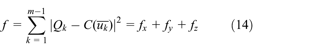
In equation (14),


where
As illustrated in Figure 5, to make gained tool path to have continuous curvature, the first and the second derivatives on the first control point and the last control point, which are named

where

The modification of fitting regions.
Then, the coordinates of


The coordinates of


To minimize


According to equation (28), equation (30) can be obtained and shown as follows

where


Therefore


where


In equations (31)–(34), Result is the value of

where


Control of fitting error
When the position of control points
As shown in Figure 6,

where


Control of fitting error.
The fitting of the tool path is an iterative process and ends when the accuracy meets the requirements of the system. If the accuracy does not meet the requirements, the fitting region is divided into two parts on the point that generates the maximum error, and the fitting progress is iteratively executed.
To have continuous curvature, the fitting regions need at least seven command points. If the divided region has less than seven command points, it would be regarded as a non-fitting region and processed by the B-spline transition method shown in section “B-spline transition method.” Assume the number of command points that locate in the fitting region is n. When the accuracy meets the requirements of the system during the first iteration, the number of the fitted B-spline curves is 1. When the tool path is smoothed all by the B-spline transition method, the number of the B-spline curves is n − 1. Therefore, the number of the fitted B-spline curves is between 1 and n − 1.
Segment of tool path
The last task before interpolation is to divide the gained tool path into velocity planning regions. First, every B-spline curve is divided into several velocity planning blocks based on the maximum of the curvature, and the data used to describe a block contain the information shown as follows:
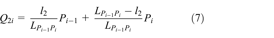
Second, the gained tool path, shown in Figure 7, is mixed with B-spline curves and line segments, so the velocity planning blocks need to be merged with the line segments. When a velocity planning block is the last block of a B-spline curve, there must follow a line segment and a velocity planning block generated by the B-spline curve that locates after the line segment. The two blocks and the line segment are merged in to one velocity planning region, and the maximum velocity allowed on the new region is updated as the minimal

The division of velocity planning regions.
Interpolation algorithm
As shown in Figure 1, when the tool path is divided into different velocity planning regions, an acceleration/deceleration control method is needed to generate the velocity profile. According to the generated velocity profile, the interpolation distance in an interpolation cycle can be obtained by integrating the velocity profile, and the position of the corresponding interpolation point can be calculated based on the tool path according to the interpolation algorithm described in section “Calculation of interpolation point.”
Look-ahead algorithm
Velocity profile
As shown in Figure 8, the jerk of the machining progress is limited, and the velocity is calculated by equation (36)


The kinematic profiles.
Look-ahead algorithm
The look-ahead algorithm, as shown in Figure 9, includes the forward planning progress and the backward planning progress. To find the maximum velocity on the end point of current planning unit, the backward velocity panning process can be described as follows: 23
Calculate the maximum velocity
Let
Let
The maximum allowable end velocity of current planning unit is
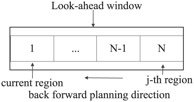
The look-ahead window.
Calculation of interpolation point
The tool path in one velocity planning region may contain a line segment and two parametric segments and have discontinuous second derivative, so the conventional interpolation parameter calculation method 24 needs to be modified when the machining path pass from the linear segment to the parametric segment and vice versa.
Assume the current interpolation point is
If

Then, the coordinates of point
If
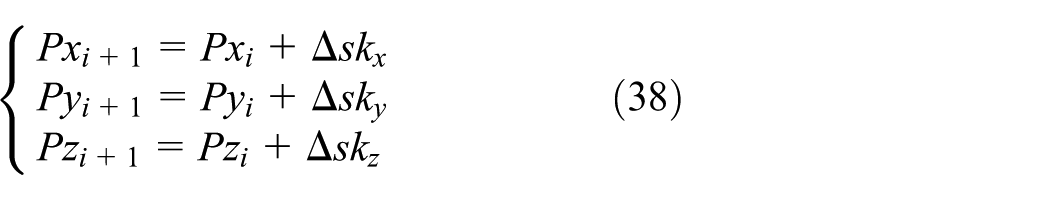
where
If the machining path in current period cross from line segment to parametric segment, the parameter
The
Simulation and experimental validations
As shown in Figure 10(a), a dolphin, having 872 command points, is used to test and analyze the performance of the proposed algorithm, while an additional experiment is implemented to make a further comparison of the actual manufacturing performance of the algorithms in three-dimensional (3D) space.

Validation of micro-line test method: (a) dolphin shape profile and (b) comparison of fitting region generated by algorithm I and algorithm II.
In the “Introduction” of this article, some existing methods to generate smoothed tool path is given, and the machining method, which uses bi-chord test method, 9 B-spline fitting method without considering the continuity of the curvature, 10 and B-spline transition method 17 is called algorithm I, while the proposed algorithm called algorithm II takes the curvature of the tool path into account.
Performance of the micro-line test method
As shown in Figure 10(b), the blue line areas denote the fitting regions generated by the bi-chord test method used by algorithm I, and the red line areas are additional regions generated by the micro-line test method used by algorithm II. Through the B-spline fitting method, the number of lines of NC codes decreases to 338 by algorithm I and 272 by algorithm II, respectively. When a fitting region could not be fitted to be a B-spline curve, it is approached by two or more B-spline curves. Compared with the bi-chord test method used in algorithm I, the new method used in algorithm II can get more fitting regions. Therefore, the effective number of NC codes is 338 and 295 by algorithm I and algorithm II, respectively, after the tool path is smoothed. It can be seen that algorithm II needs less amount of command lines and effectively reduces data quantity of NC codes.
As the NC codes used to describe the whole tool path which is shown in Figure 10(a) is large, the tool path expressed by solid line, which contains 107 command points, is marked by the rectangle in Figure 10 and selected to validate the performance of different algorithms in the following paper, and the processing results are shown in Figure 11.

Comparison of processed tool path: (a) original tool path and the new tool path gained by algorithm I, (b) original tool path and the new tool path gained by algorithm II, (c) curvature curve of the new tool path gained by algorithm I, and (d) curvature curve of the new tool path gained by algorithm II.
Figure 11(a) and (b) shows the new tool path gained by the algorithm I and algorithm II, respectively, and the blue circle represents the control points of the B-spline curves which are used to approach the fitting regions of the tool path. Figure 11(c) and (d) shows the curvature curves of the new tool path. According to Figure 11, two results could be found: First, the new tool path gained by algorithm II has two regions fitted into B-spline curves, while the tool path gained by algorithm I has only one region fitted into B-spline curve. Second, the curvature curve of the tool path generated by the algorithm I is not continuous at starting point and ending point of the fitted B-spline curve, while the curvature curve of the tool path generated by the algorithm II remains continuous on the whole tool path.
Contrast to the method used in algorithm I, the simulation results indicate that algorithm II reduces the amount of NC codes and generates more smoothed tool path with continuous curvature. The more smoothed tool path generates higher machining speed and less fluctuation of acceleration and contributes to better machining quality.
To test the machining efficiency of the algorithms, the kinematic profiles are given. In the simulation, the specified feed rate velocity is 9 m/min, the maximum acceleration is 0.3 m/s2, the maximum jerk is 50 m/s3, and the sample time is set to be 0.002 s. The kinematic profiles are shown in Figure 12.

The kinematic profiles: (a) feed rate profile, algorithm I; (b) feed rate profile, algorithm II; (c) acceleration profile, algorithm I; (d) acceleration profile, algorithm II; (e) jerk profile, algorithm I; and (f) jerk profile, algorithm II.
In Figure 12(a) and (b), the velocity planning segments are divided by the red lines. The B-spline curves generated by the fitting method could be divided into longer velocity planning segments than curves generated by the transition method, so Figure 12(a) has 45 velocity planning segments, while Figure 12(b) only has 38 velocity planning segments.
As shown in Figure 12(c) and (d), the longer velocity planning segments make the acceleration profile to have less fluctuation, especially during the time 0.3 and 0.6 s. Combined with the continuous curvature profile, the longer and fewer velocity planning segments make the machining velocity become higher. As illustrated in Figure 12(a) and (b), the machining time needed by the algorithm I is 0.904 s, while algorithm II only needs 0.878 s.
Experimental results
To verify the performance of the proposed algorithm, the tool path shown in Figure 10(a) is implemented on SMTCL VMC850E machining center, which is equipped with an open CNC system developed by the authors. 25 The carving material is 7075-T7451 aviation aluminum. 26 The specified feed rate is 9 m/min, the maximum acceleration is 5 m/s2, the maximum jerk is 50 m/s3, and the sample time of the CNC system is 0.002 s.
Figure 13(b) is the machining results. In Figure 13(b), the algorithm which uses circle transition method 13 to smooth the tool path is named the traditional algorithm. To show the machining results clearly, parts A and B marked in Figure 11(b) are enlarged and shown in Figure 14.

The machining center and machining results: (a) SMTCL VMC850E machining center and (b) comparison of actual machining results.

The actual machining results: (a) part A in Figure 10(a), traditional algorithm; (b) part A in Figure 10(a), algorithm I; (c) part B in Figure 10(a), algorithm I; and (d) part B in Figure 10(a), algorithm II.
The part A in Figure 11(a) is a non-fitting region and Figure 14(a) and (b) is the partial enlarged views of the machining results of part A in Figure 11(a). Figure 14(a) is the machining result of the traditional algorithm, while Figure 14(b) is the machining result of algorithm I.
Part A is a non-fitting region, so circle transition method and B-spline transition method are used by the traditional algorithm and algorithm I, respectively, to smooth the tool path. As having continuous curvature on the processed tool path, the machining quality of algorithm I is better than the traditional algorithm.
The part B in Figure 11(a) is a fitting region, and Figure 14(c) and (d) is the partial enlarged views of the machining results of part B. Figure 14(c) is the machining result of algorithm I, while Figure 14(d) is the machining result of algorithm II. Taking continuous curvature into account in the fitting of the fitting regions, algorithm II makes the curvature of the processed tool path continuous, shown in Figure 11(d), so the acceleration profile of the machining process is continuous. Contrast with algorithm II, the curvature of the processed tool path gained by the algorithm I is discontinuous, shown in Figure 11(c), which would result a sudden change in the acceleration profile. The continuous acceleration profile not only contributes to less machining time, shown in Figure 12, but also reduces the shock of the machine tools, so the machining quality of algorithm II shown in Figure 14(d) is better than the machining quality of algorithm I shown in Figure 14(c).
The detailed machining information is given in Table 1.
Detailed machining information.

NC: numerical control.
As shown in Table 1, algorithm I needs less machining time and less amount of NC codes than the traditional algorithm, while algorithm II has the same advantages when compared with algorithm I.
Therefore, the actual machining results verify the conclusions in section “Performance of the micro-line test method”: algorithm II can reduce the amount of NC codes, improve machining efficiency and generate better machining surface quality.
Experiments in 3D space
Having the functions of five-axis transformation, rotation tool center point control (RTCT), and 3D radius compensation, the LT series CNC systems developed by the authors 25 are able to machine the workpiece in 3D space and make us only need to focus on the control of cutter location. Integrating algorithm I and algorithm II into the CNC system, an engine blade is implemented on SMTCL HTM63150iy five-axis machining center, shown in Figure 15(a), to test the performance of the algorithms in 3D space. The carving material and the parameters of the system are the same with the experiment in section “Experimental results,” and the machining process is shown in Figure 15(b).

The machining of engine blade: (a) SMTCL HTM63150iy and (b) machining process.
As the shape of the blade is symmetrical, the left part of the blade is machined by algorithm I, while the right part of the blade is machined by algorithm II. The machining result is shown in Figure 16(a).

Machining result of engine blade: (a) machining result; (b) part A of the machining result, algorithm I; and (c) part B of the machining result, algorithm II.
The machining time of the left part and the right part is 169 min and 56.242 s and 154 min and 20.488 s, respectively; the machining time indicates that algorithm II has much higher machining efficiency than algorithm I.
In Figure 16(a), the most significant differences of the machining result are marked with red circle. The part A is machined by algorithm I, while the part B is machined by algorithm II. Part A is symmetrical with part B, and the enlarged views of parts A and B are shown in Figure 16(b) and (c), respectively. It can be seen that algorithm II generates better machining result than algorithm I. This experimental result further validates the effectiveness of the proposed algorithm in obtaining higher machining efficiency and generating better machining quality.
Conclusion
In this article, a smooth tool path generation and real-time interpolation algorithm based on B-spline curves is proposed. The algorithm distinguishes the NC command points into fitting regions and non-fitting regions and employs B-spline to gain smooth tool path. The seven-phase velocity scheduling profile and modified interpolation parameter calculation method are used to improve the surface quality.
In contrast with previous works, the proposed algorithm has two advantages: (1) the proposed algorithm needs less data amount to express the tool path. (2) The gained tool path has continuous curvature and could achieve higher machining speed and get better machining surface quality.
Simulations are conducted to make two comparisons: the comparison between the bi-chord test method and the micro-line test method and the comparison between the original tool path and the tool path gained by algorithm I or algorithm II. Simulation results demonstrate that the proposed algorithm can generate smoother tool path that takes less amount of NC codes and has continuous curvature which contributes to increased machining efficiency and improved machining quality. One dolphin shape and one engine blade are machined by the machining center. Experimental results validate the simulation conclusions: the proposed algorithm can generate satisfied machining surface quality and reduce machining time and data amount.
Footnotes
Handling Editor: Xichun Luo
Declaration of conflicting interests
The author(s) declared no potential conflicts of interest with respect to the research, authorship, and/or publication of this article.
Funding
The author(s) disclosed receipt of the following financial support for the research, authorship, and/or publication of this article: This work was supported by a Project of Shandong Province Higher Educational Science and Technology Program (grant no. J17KA038) and the High-End CNC Machine Tools and Basic Manufacturing Equipment, National Science and Technology Major Projects (grant no. 2016ZX04004006).