
Abstract
In this study, a real-time look-ahead interpolation methodology with B-spline curve fitting technique using the selected dominant points is proposed. First, an improved scheme for selecting the dominant points is proposed to reduce the numbers of control points and iterations. Second, a point-to-curve distance function is defined, and its Taylor’s expansion is investigated for curve fitting. Finally, a real-time look-ahead interpolation function, which consists of spline fitting, feedrate scheduling and parametric interpolation modules, is developed to obtain smooth tool path and feedrate profile simultaneously. Experiments on an X-Y-Z platform are conducted with a three-dimensional tool path, and the results demonstrate the feasibility and efficiency of the present algorithms.
Keywords
Introduction
Nowadays, short line segments, or G01 blocks, are still the most widely utilized representation form for the tool paths in the computer numerical control (CNC) machining. However, due to the tangency and curvature discontinuities, frequent feedrate fluctuation and acceleration variation may occur at the junctions of adjacent segments during the linear interpolation, which inevitably deteriorate the machining efficiency and quality. Many studies show that the parametric interpolation methods can realize high-feedrate and high-accuracy machining.1–3 Thus, a solution for the aforementioned problem is to convert the short line segments to B-spline curves in a real-time manner and apply parametric interpolation method in the CNC system. In such case, there are two major concerns related to the curve fitting: (1) selection of the discrete points and (2) B-spline curve fitting to the selected points.
There are two approaches to convert the linear segments to parametric splines, that is, the interpolation method and the approximation method. For the interpolation method,4–8 the resultant number of the control points equals that of the discrete points. If numerous line segments are involved, the storage requirement and computational load for the curve fitting process are considerably huge. Compared with the interpolation method, the approximation method can describe the fitted B-spline curve with fewer control points,9–12 which means the curve information can be compressed significantly. Some commercial CNC systems already provide curve approximation functions, such as nano smoothing in FANUC 32i 13 and COMPCAD in Siemens 840D. 14 However, because the required number of the control points is unknown in advance, the aforementioned approximation methods should select some arbitrary points and then adopt an iterative process to adjust both the number and locations of the control points for the fitted curve. Thus, the number of the control points and iterations may be large, which requires considerable computational efforts. To solve this problem, the technology such as feature recognition can be adopted.15,16 Recently, Park and Lee 17 proposed a novel dominant point selection scheme, which chooses the feature points of the curve for B-spline curve fitting. With this method, better curve approximation can be achieved with far fewer control points. Park 18 then expanded the idea of dominant points and proposed a B-spline surface fitting method according to the dominant columns along two directions. However, the existing dominant selection schemes merely consider the curvature factor. In their practical applications, numerous iterations are required to add new dominant points, which degrade the real-time performance.
Based on the selected discrete points, the approximation algorithm using the least-square (LS) optimization technique is usually adopted to generate the fitted B-spline curves. The aforementioned studies employed point distance minimization (PDM) method to approximate the discrete points, which minimizes the squared distance between the discrete point and the point on the fitted curve. Actually, the target of the approximation method is to pursue a B-spline curve and keep the distance between the line segments and the fitted spline curve within a specified tolerance. Obviously, the traditional PDM method may lead to unsatisfied approximation results. To solve this issue, Blake and Isard 19 defined the distance from the discrete point to the tangential line at the corresponding point as the point-to-curve distance and proposed a tangent distance minimization (TDM) method. Wang et al. 20 proposed a curvature-based quadratic approximant of squared distance between the point and the fitted curve and employed the distance in the squared distance minimization (SDM) method. However, the existing TDM and SDM methods only apply to planar curves.
In this study, a new selection scheme for dominant points and a new SDM method based on the point-to-curve distance function are proposed, which can apply to spatial line segments and produce a fitted B-spline curve with fewer control points and higher convergence rate. The remainder of this article is organized as follows. In section “Cubic B-spline curve fitting,” a novel dominant point selection scheme is presented to reduce the number of control points and iterations. Also, a point-to-curve distance function is defined and its differential property is investigated, and then its Taylor’s expansion is used for SDM optimization. Moreover, the Hausdorff distance is adopted as a criterion for the approximation accuracy, and an accuracy control method is presented. In section “Real-time look-ahead interpolation with spline fitting,” a real-time look-ahead interpolation program, which consists of spline fitting, feedrate scheduling and parametric interpolation modules, is presented. Experiments are conducted in section “Experimental validations,” and the conclusions are given in section “Conclusion.”
Cubic B-spline curve fitting
Selection of dominant points
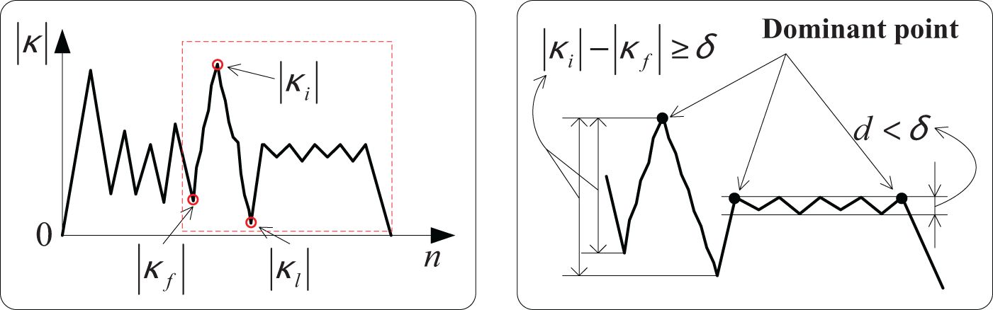
The proposed dominant point selection scheme takes three steps: selection of local curvature maximum (LCM) points and two end points, determination of the points where the bending direction of the curve changes and selection of the chordal points. The curvature provides useful information to characterize the shape of the curved path. Thus, it is natural to use the discrete curvature information to determine the dominant points15,16 for the line segments, which can be estimated by the curve fitting methods.21–23 In such case, the curvature may fluctuate because of the trajectory discretization and the curvature evaluation error, as shown in the dashed box in Figure 1, where
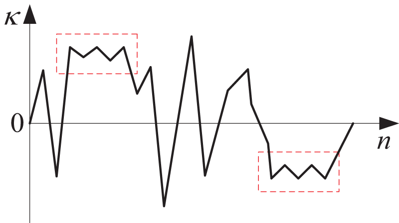
Dominant point selection based on the curvature information.
To solve this problem, an improved selection scheme for the LCM points is proposed. First, given a set of ordered discrete points
where
Discrete curvature for the short line segments.
Then, the two end points
Proposed LCM point searching scheme: (a) curvature profile and (b) the details in the dashed box of the left sub-figure.
The sign of the discrete curvature changes as the bending direction of the curve changes. The corresponding points are denoted as curvature-passing-zero (CPZ) points. Obviously, point
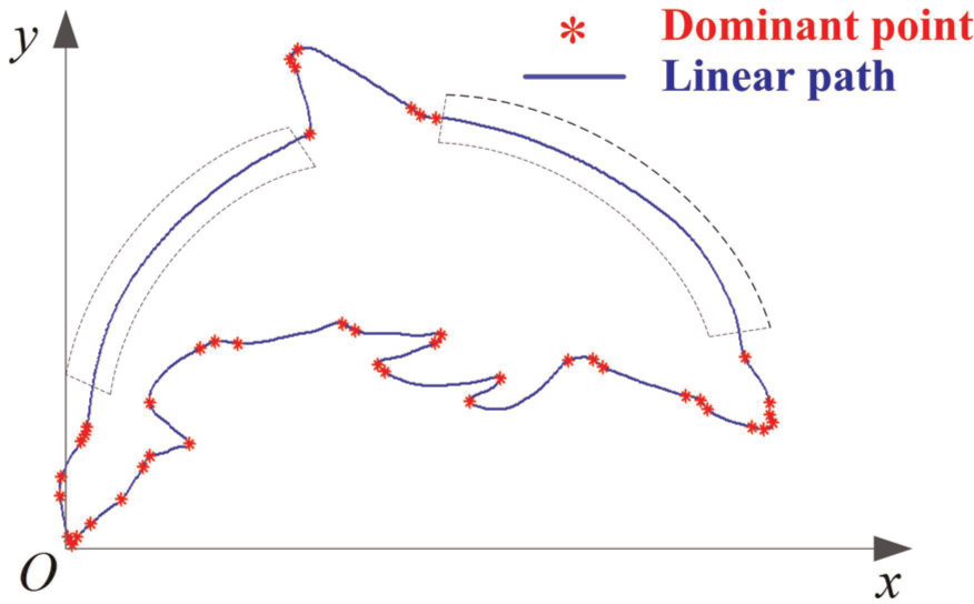
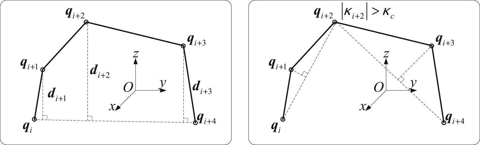
Although the LCM points can reflect the sharp regions of the linear curved path, these points fail to cover the total shape of the curve. Taking the dolphin curve as an example, as shown in Figure 4, no dominant points are selected within the dashed boxes because the curvatures vary slightly. Clearly, the chosen dominant points cannot reflect the curve shape in such regions. To guarantee the fitting process to converge, new dominant points need to be added iteratively. To decrease the iteration number, dominant points in such regions are also required. In the following, the chordal points, which are selected as another kind of dominant points, are searched according to the chord scanning.
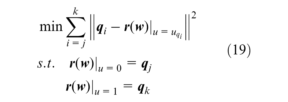
Reason for the selection of the chordal points.
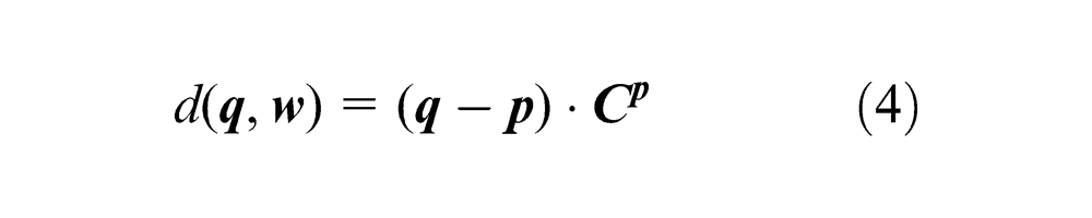
As shown in Figure 5,
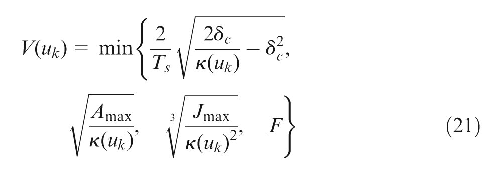
Selection scheme for chordal points: (a) chord scanning and (b) iterative subdivision.
Procedure 1
Selection of the chordal points:
Step I. Calculate the chordal deviation
Step II. Calculate the curvature of point
By employing the proposed scheme, the dominant points are also selected at the flat regions of the curve. In addition, the dominant points are thicker at the sharp regions, which can describe the curve more accurately in such regions.
Point-to-curve distance function and its application to spline fitting
Zhu et al. 24 defined a signed point-to-surface distance function and applied its second-order Taylor’s expansion to the approximation for the target surface. By expanding the idea, this study defines a point-to-curve distance function and investigates its differential properties as well. Taylor’s expansion of the distance function is then utilized in the B-spline curve approximation.
Definition 1 (point-to-curve distance function)
Given a regular smooth curve

where

As shown in Figure 6,
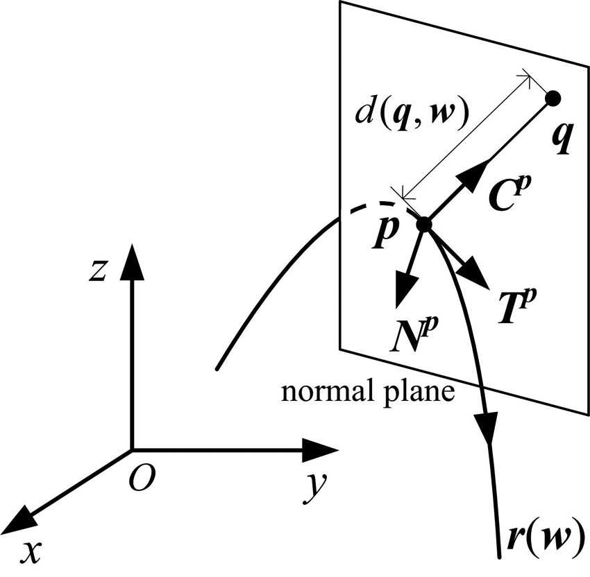
Point-to-curve distance function.
and
where
For the point-to-curve distance function
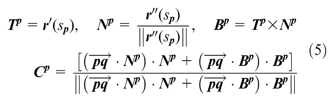
Proposition 1. Let
where
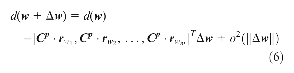
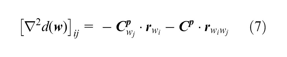
Proposition 2. For the regular smooth curve
where
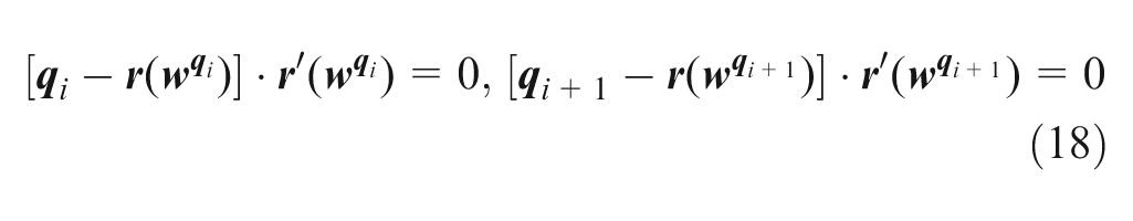
The proofs of both propositions are given in Appendix 1. According to equations (6) and (7), the second-order Taylor’s expansion of
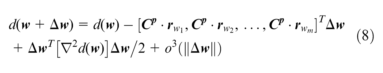
For planar curves, equations (6) and (8) can be rewritten as
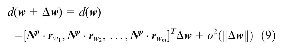
and
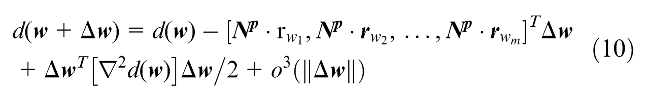
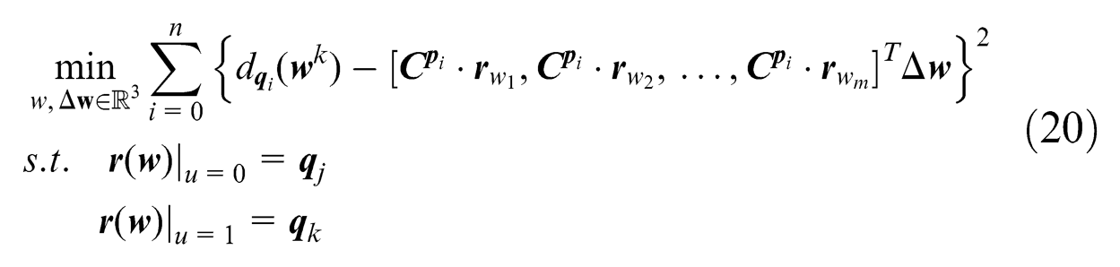
Clearly, the value of

where
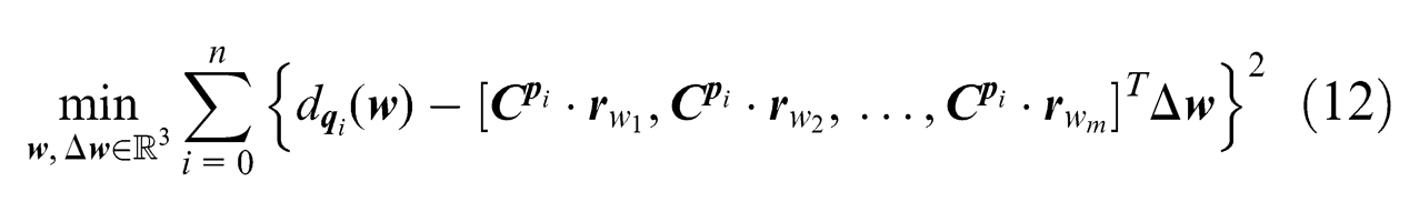
where
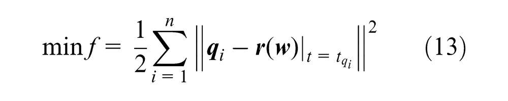
Equation (12) is the proposed SDM method in this study. Furthermore, the distance between the given point set
Note that if the discrete points are far away from the fitted curve, the proposed method inevitably introduces huge approximation error. Thus, a proper initial B-spline fitting curve is necessary. The traditional PDM technique can be utilized to obtain such an initial B-spline curve
where
Procedure 2
The proposed SDM method:
Step I. Given a set of discrete points
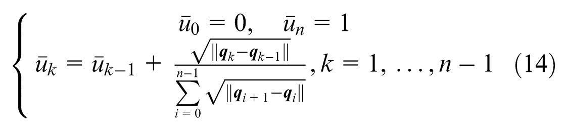
Compute the parameter values of all the discrete points by performing chord length parameterization 27
Select the initial dominant points according to the scheme introduced in section “Point-to-curve distance function and its application to spline fitting.”
Perform knot placement. The knots are determined by averaging the parameters of the dominant points, which can be expressed as 25
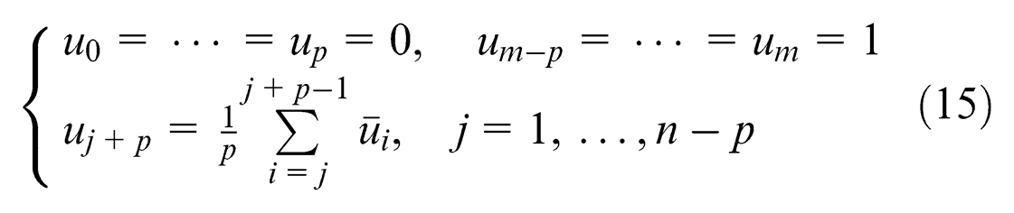
where
The PDM method (equation (13)) is utilized to approximate the dominant points, and a fitted B-spline curve
Step II. Update the initial B-spline curve to get the target fitted curve.
5.
Check the deviation between the fitted curve
6.
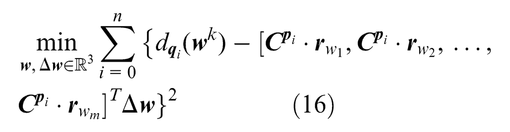
Solve the following problem to determine the differential increment of the control points
7. Update the control points
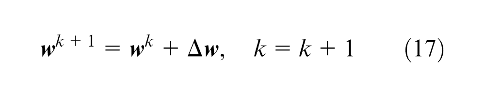
8. Check the deviation again, if
9. If the fitting accuracy is not satisfied within some regions defined by two adjacent dominant points, choose the point with the maximum error as the new dominant point. Subsequently, perform knot placement according to the updated dominant points, and go to step 3.
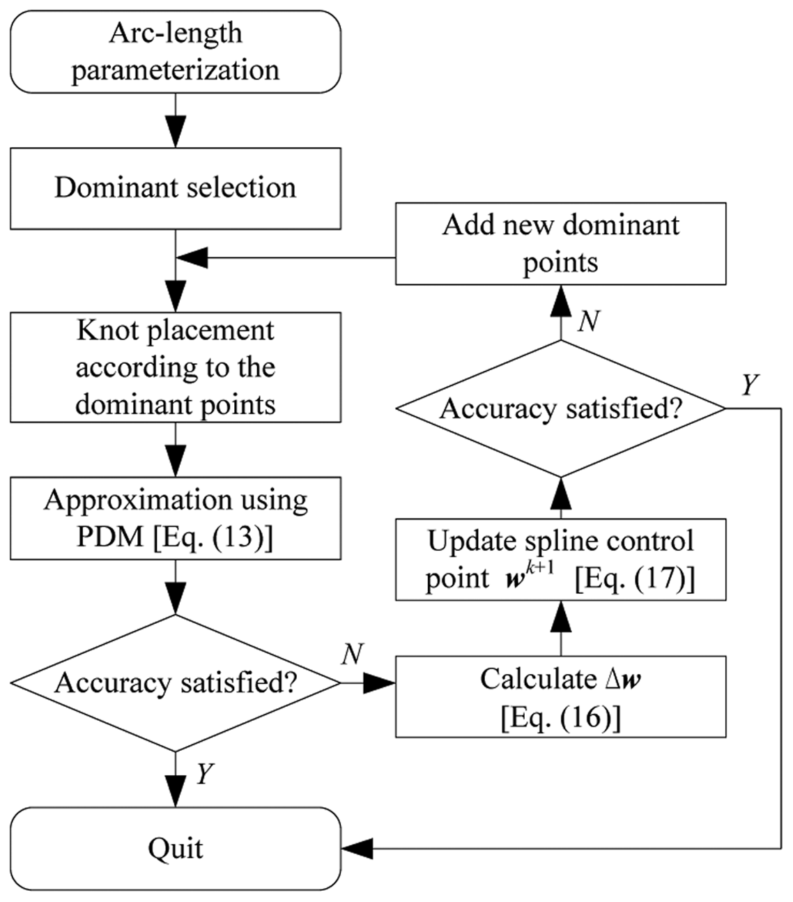
The flowchart of the proposed SDM method is shown in Figure 7. The accuracy control method in the spline fitting process is presented in the following.
Flowchart for B-spline curve fitting.
Accuracy control in spline fitting
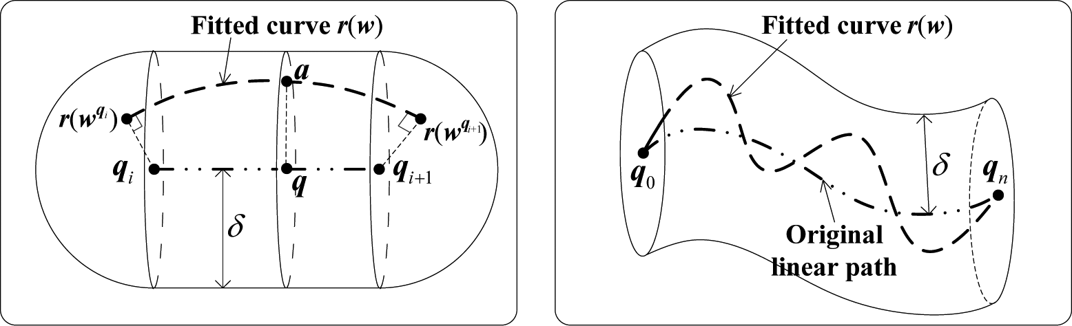
The B-spline fitting method should keep the distance between the linear segments and the fitted B-spline curve within a specified tolerance. The Hausdorff distance is usually adopted as a criterion for the resultant approximation quality, which is defined as follows.
Definition 2 (Hausdorff distance)
Given two non-empty subsets
Obviously, it is difficult to compute the Hausdorff distance directly. Thus, the verification process is simplified according to the following definition and proposition.
Definition 3 (Hausdorff envelope)
As shown in Figure 8(a), the Hausdorff envelope (HE) of the line segment
Accuracy control for B-spline curve fitting: (a) Hausdorff envelope for line segment and (b) accuracy control for the fitted control.
Proposition 3. As shown in Figure 9, let the foot points of
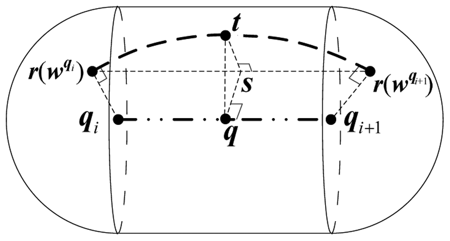
Line segment and its Hausdorff envelope.
Actually, the control points mainly affect the shape of the fitted curve. Thus, to verify that the fitted curve
Procedure 3
Hausdorff distance verification:
Step I. Calculate the foot points
Step II. Check if
Step III. Evaluate the center points of
Real-time look-ahead interpolation with spline fitting
In this section, an interpolator with real-time look-ahead interpolation function is proposed, which consists of three modules: spline fitting, feedrate scheduling and parametric interpolation modules. Figure 10 illustrates the flowchart of the look-ahead interpolation and motion control. Considering the CPU’s capability, the look-ahead period is set to be 4 ms to guarantee that the spline fitting and feedrate scheduling can be finished within one sampling interval.
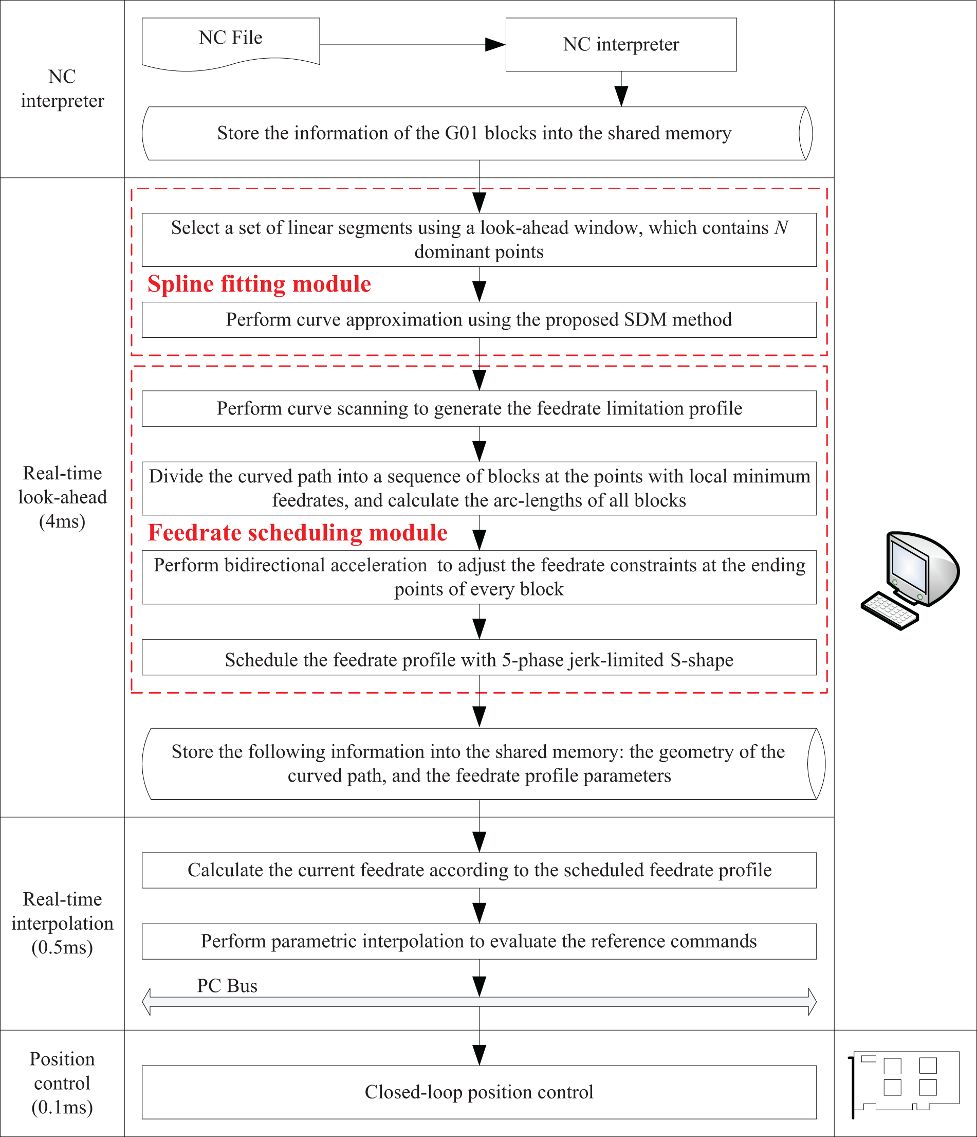
Flowchart of the look-ahead interpolator and motion controller based on B-spline approximation.
Spline fitting module
Note that the most time-consuming part of the approximation task is to solve the linear optimization problem, which is expressed in equation (16). If too many dominant points are involved within one look-ahead period, the considerable computational load of the fitting process may exceed the processor’s capability. To guarantee the real-time performance of the look-ahead interpolation, a floating window is employed to determine the number of the line segments handled in one look-ahead period. At the beginning of every look-ahead timer interrupt response routine, N dominant points are detected and then the involved line segments are applied for curve fitting.
In every floating window, a B-spline curve is generated. To avoid variation at the junctions of two adjacent fitted B-spline curves, the condition of C 0 continuity is added into the fitting algorithm. Thus, by utilizing the PDM method to yield the initial B-spline, equation (13) is rewritten as
where
Then, using the proposed SDM method to update the B-spline, equation (16) is rewritten as
In one look-ahead period, the geometric information of the B-spline curve in the next period is unknown in advance. Thus, in this study, only C 0 continuity rather than the higher-order continuity is employed.
Feedrate scheduling and parametric interpolation modules
Four steps are involved in the feedrate scheduling and parametric interpolation modules, the details of which are summarized as follows.
Procedure 4
Feedrate scheduling and parametric interpolation:
Step I: curve scanning. In the first step, the fitted curve is scanned to obtain the initial feedrate limitation profile. During the curve scanning process, pre-interpolation is performed, and the feedrate constraint at each scanning step is determined by
where
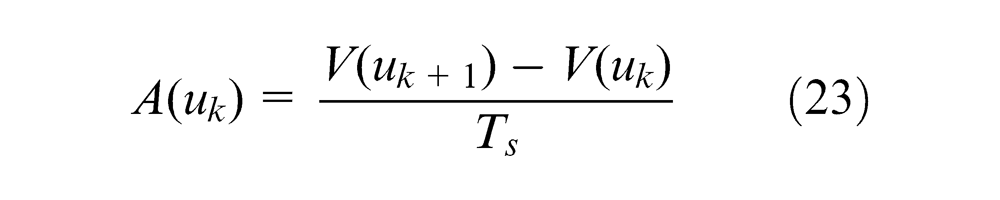
Then, the second-order Taylor’s expansion with respect to the time can be employed to approximate the curve parameter
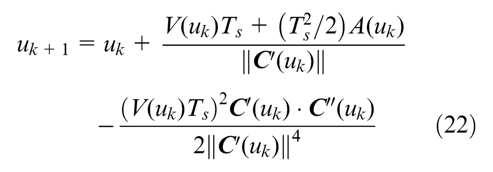
where
The feedrate minimum points, whose curvatures satisfy the following expression, are treated as the junctions of acceleration and deceleration blocks
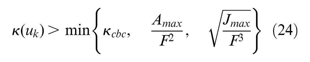
where
Note that the feedrate limitations within a look-ahead window can be evaluated by equation (21), but those at the junctions of adjacent fitted B-spline curves cannot use this concept because the curvature is not continuous. To solve this problem, the tangential lines of the two B-spline curves are used to approximate the splines, as shown in Figure 11. The feedrate limitation is determined by
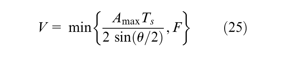
Connection of two fitting curves in two look-ahead floating windows.
Step II: Bidirectional acceleration. In the second step, bidirectional acceleration is implemented within the floating look-ahead window. The aim is to correct the feedrate constraints at the junctions of the acceleration and deceleration blocks. Considering the constraints of tangential acceleration and jerk, S-shape acceleration is performed in both the forward and backward directions, and the feedrate limitations are corrected. Readers can refer to Zhao et al. 29 for detailed description about the bidirectional acceleration.
Step III: Acceleration/deceleration (ACC/DEC) planning. With respect to the obtained feedrate limitation profile, a jerk limited S-shape feedrate profile is planned to avoid shock or vibration at the sharp corners or positions without continuous curvature. Readers can refer to Lin et al. 2 for more detailed descriptions about the feedrate scheduling.
Step IV: Parametric interpolation. Finally, with the feedrate profile obtained from the look-ahead function, the interpolator performs parametric interpolation to generate the reference position commands and sends them to the motion controller for position feedback control. The traditional Taylor’s expansion is adopted as the interpolation method, as shown in equation (22).
Experimental validations
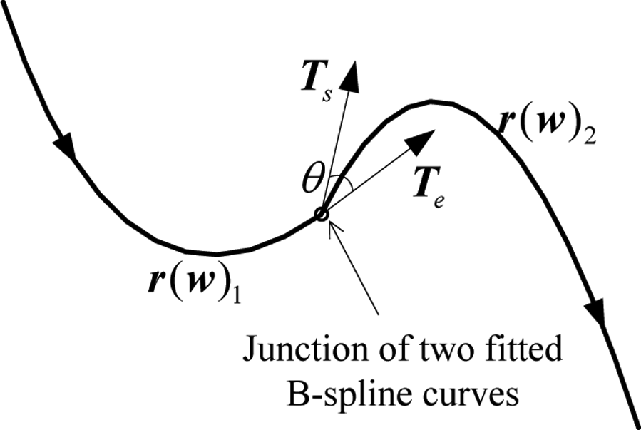
To demonstrate the proposed B-spline curve fitting method, experiments are conducted on a triaxial platform, as illustrated in Figure 12. The experimental system contains three main parts: a PC, which is employed to perform the look-ahead interpolation; a custom motion control card, which is equipped with a fixed-point TMS320F2812 DSP to perform closed-loop position control and an X-Y-Z table, which is driven by three YASKAWA SGDV series servo drivers and SGMJV motors. The built-in incremental encoder for each motor is used for position feedbacks. The resolution of the encoder is 10,000 pulses/rev. The lead of the ball screws for the X-Y-Z table is 10 mm/rev.
Layout of the experimental platform.
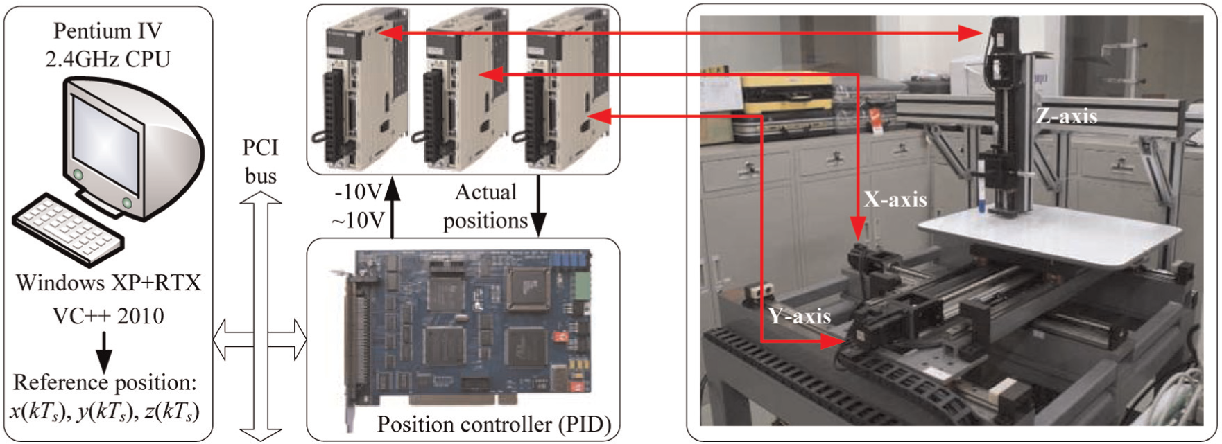
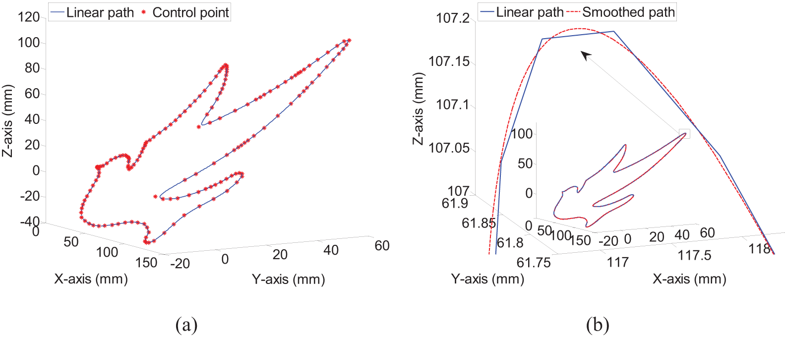
A three-dimensional (3D) pigeon-shaped linear tool path with 1270 line segments, which is generated by UGNX, is applied to validate the proposed dominant selection scheme and SDM method. The maximal acceleration
Three steps are involved in the experiments. First, two dominant point selection schemes, including the proposed method and Park’s method, are performed for the linear tool path. Figure 13(a)–(d) illustrates the distribution of dominant points on the original line segments and curvature profiles, respectively. From Figure 13(a), it can be found that the dominant points determined by the proposed method are adaptively selected more at the complicated regions but fewer at the flat regions. In addition, the proposed method can characterize both the sharp and flat shapes simultaneously. On the contrary, without filtering the discrete curvatures, numerous dominant points are selected at the regions where the points have almost the similar curvatures using Park’s method, as shown in Figure 13(b) and (d).
Distribution of the dominant points on the curved path and curvature profile using the two methods: (a) result of the proposed method, (b) result of Park’s method, (c) result of the proposed method and (d) result of Park’s method.
Second, the proposed SDM method is applied on the basis of the selected dominant points with above two methods. In this study, the dominant point number specified in one look-ahead window is 30. Figure 14 illustrates the fitting results using the proposed dominant point selection scheme and the proposed SDM method.
Fitting result using the proposed dominant point selection scheme and SDM fitting method: (a) layout of the control points and (b) fitting result.
Table 1 summarizes the detailed numerical results of three different B-spline curve fitting methods: Park’s dominant point selection scheme with the proposed SDM method, commercial software tool UGNX and the proposed dominant point selection scheme with the proposed SDM method. It can be seen that compared with Park’s method, the proposed one can reduce the control points by 25.82% with only two iterations. Compared with UG, the proposed method can reduce the control points by 19.39% using cubic B-spline, which can achieve C 2 continuity. In addition, compared with the original linear tool path, the fitted curve can describe the profile with 158 control points, which indicates that the curve information is compressed significantly.
Comparison of the fitting results using three methods.
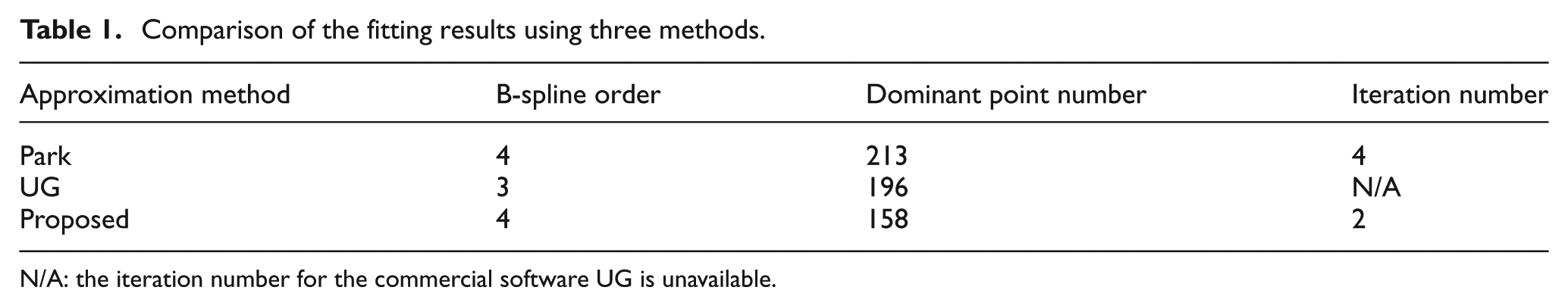
N/A: the iteration number for the commercial software UG is unavailable.
Then, the proposed dominant selection scheme and the PDM method are applied for B-spline curve fitting. The resultant numbers of control points and iteration are 182 and 3, respectively. From Table 1, it can be seen that the proposed SDM method can reduce control points by 13.19% and iteration by 1 time compared with the PDM method. Thus, the proposed SDM method can not only reduce the control points effectively but also increase the convergence rate.
Third, curve scanning, bidirectional acceleration and ACC/DEC planning are performed with respect to the fitted B-spline curves. Figure 15 shows the generated feedrate scheduling profiles for the original tool path and the fitted curve. Compared with the original linear curved path, it can be found that the fitted curve significantly increases the machining efficiency. The elapsed time for the interpolation with two methods is 19.17 and 7.48 s, respectively. This means the parametric interpolation improves the productivity by 60.98% as compared with the original linear interpolation method.
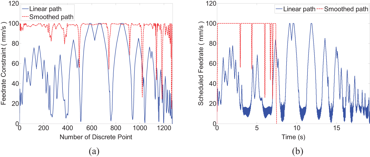
(a) Feedrate limitation and (b) scheduled profiles for the original linear tool path and the fitted tool path.
Conclusion
In this article, a real-time look-ahead interpolation with B-spline curve approximation technique for short line segments is proposed. Compared with the traditional approximation methods, the proposed method has the following advantages: (1) an adaptive dominant point selection scheme is proposed, which can reduce the number of the control points and the iteration for the fitting procedure and (2) a point-to-curve distance function is defined and utilized for SDM, which can be utilized in 3D approximation with higher convergence rate.
Experiments are conducted on an X-Y-Z table. The results demonstrate the effectiveness of the proposed method in CNC machining of 3D short line segments.
It is worth mentioning that only C 0 continuity is achieved at the junctions of two adjacent fitted curves, and the curve fitting method cannot be directly applied to generate dual B-spline curves for five-axis machine tools. Our future works will focus on improving the continuity and investigating the dominant point–based dual B-spline curve fitting method.
Footnotes
Appendix 1
Appendix 2
Declaration of conflicting interests
The authors declare that there is no conflict of interest.
Funding
This work was partially supported by the National Natural Science Foundation of China under grant No. 51325502, the National Key Basic Research Program under grant No. 2011CB706804 and the Science & Technology Commission of Shanghai Municipality under grant No. 13JC1408400.