Sage Journals: Discover world-class research

Abstract

The calculation method of cutter location (CL) points only considers the geometric errors, but cannot consider the requirements of the corner transition algorithm in CNC, which results in the smoothing algorithm in the CNC not playing a maximum role or even failing. To solve this problem, a calculation method of the CL points considering corner transition speed in CNC is proposed. Firstly, the key geometric parameters of the CL points that affect the corner speed are analyzed. Secondly, according to the analysis results, the objective function is established to connect the CL points calculation in CAM and the corner transition speed in CNC. By solving the objective function, the calculation method of the CL points is developed. Finally, the effectiveness of this method is verified by experiment. Comparing with the commonly used iso-chord height method, the proposed method can increase the speed at the corner of the CL points and reduce the acceleration and jerk at the same time. By the proposed method, the tracking accuracy, trajectory accuracy, and machining efficiency can be significantly improved. The proposed method can be integrated into CAM software to generate high quality CL points.

Keywords

Cutter location (CL) points corner transition algorithm NURBS curve corner speed

Introduction

There are many factors that affect the machining efficiency and quality of sculptured surface parts. These factors exist in all aspects of the data flow of the machining process,¹ including the tool paths and the CL points generated by CAM,² the setpoints interpolated by the CNC system, the dynamic errors caused by servo control, the static/quasi-static errors of mechanical structures, the deformation and chatter during cutting, etc. Among all these factors, the CL points generated by CAM are located upstream of the data flow. Therefore, generating high-quality CL points is the first step to achieving high machining accuracy and efficiency.³

The CL points are generated through preprocessing in CAM. First, the machined surface is discretized into the tool paths. Then, the CL points are generated by discretizing the tool paths. Classical tool path generation methods include iso-parametric, iso-planar, and iso-scallop methods etc. The iso-parametric method^4–9 is aimed at parametric surfaces. This method keeps one parameter of the surface constant, while the other parameter changes incrementally at regular intervals. The iso-planar method^10–13 uses the intersection line obtained by the equidistant section plane and the machined surface section as the tool path. The distance between the planes is mainly determined by the scallop height requirements. The iso-scallop method^14–17 sets an initial tool path on the surface. The adjacent tool path is calculated by keeping the scallop height between adjacent tool paths as a constant value. It can be seen from above research that the tool paths generated by these methods were all constrained by the scallop height to ensure the geometric accuracy of the part surface.

Under the scallop height constraint, the machining efficiency can be improved by optimizing the tool path direction. Marciniak¹⁸ and Kruth and Klewais¹⁹ studied the relationship between the tool path direction and machining efficiency, which was substantially improved by changing the toolpath. Kim and Sarma²⁰ proposed a time optimal tool path generation method. Chiou and Lee²¹ proposed a machine potential field approach to generate five-axis machining tool paths. Giri et al.²² find that when the initial tool path is along the direction of maximum curvature, the machining time is significantly reduced.

Besides improving machining efficiency, considering the tool path direction can bring more benefits. Yao et al.³ proposed a tool path regeneration method, and the results showed that the average error of their generation method was significantly reduced. Meng Lim and Menq²³ proposed a cutting-path-adaptive-feed rate tool path generation method with the constraints of surface geometric accuracy and tool deformation, which can simultaneously improve productivity and product quality for sculpted surface production. Lu et al.²⁴ developed a method of tool path generation for the twin-tools milling process of gas turbine blades. By the method, the deformation of a blade caused by cutting force is obviously reduced compared with a conventional machining process with a single tool. The direction of the tool path affects the feed rate of each axis, which is the main parameter that affects the tracking error and contour error. Considering the influence of the tool path direction on the tracking error and the contour error, Lu et al.²⁵ established a contour error-oriented tool path generation method. The results showed that the contour error of the generated toolpath under the optimal cutting direction was much smaller than the contour error in other cases.

To sum up, as the upstream of the data flow, the tool path generated by CAM no longer only considers geometric accuracy, but increasingly considers the downstream of the data flow such as cutting process and machine tool performance.

After the tool paths are determined, the CL points are generated by discretizing the tool path according to the geometric errors such as chord height error. By discretizing, the tool path are widely represented as the form of continuous short line segments.²⁶ This form of the tool path is only C0 continuous which causes the sudden change of speed and mechanical vibration and prolongs the machining time. In order to solve these problems, the continuous short line segments tool paths are usually smoothed by the CNC systems.

The common tool path smoothing algorithms include global smoothing and local smoothing.²⁶ The global smoothing algorithm uses quartic Bezier curve,^27,28 quintic B-spline curve,²⁹ Akima curve³⁰ etc. to fit all CL points. However, global smoothing has a large number of fitting points, resulting in a large amount of calculation. Instead, local smoothing is more widely used in practice, because it works on the corner of two adjacent line segments. Bi et al.³¹ used cubic Bezier curves to smooth the corners of adjacent line segments, and the method was effective in increasing the feed rate and producing smoother velocity and acceleration profiles. Shi et al.³² used the PH curve to smooth the rounded corners and solved the problem of discontinuous tangent and curvature at the corners. Tulsyan and Altintas³³ inserted a quintic spline at the junction of two line segments to achieve C3 continuity. Huang et al.³⁴ proposed a real-time G2 continuous local smoothing method by replacing the corners of the CL points and tool orientation paths with cubic B-splines. Lin et al.³⁵ proposed a local corner smoothing method considering kinematics and real-time constraints while considering axial jerks during corner smoothing and the tangential pull of the tool blade to ensure the surface quality of the part.

However, because the generation method of CL points only considers geometric errors such as chord height error, this method is still in a state of separation from the downstream data flow at present. Furthermore, in the current state of separation of CAM and CNC, the generation of CL points in CAM does not consider the requirements of the downstream CNC smoothing processing, which results in smooth processing in CNC not playing a maximum role or even failing.

The smoothing of CL points is completely done in CNC by the corner transition algorithm. In CNC, the transition algorithms increase the corner speed according to the inserted transition curve and the geometric parameters of adjacent line segments. So, the smoothing effect is not only related to the fitted curve, but also the geometric parameters of the CL points. It is supposed that the machining efficiency and the machining quality should be further improved as long as the requirements of the CNC corner transition on the geometric parameters of the CL points are integrated into the CAM.

Consequently, the purpose of this study is to establish the calculation method of CL points considering the CNC corner transition algorithm. Firstly, the key geometric parameters of CL points that affect the corner speed are analyzed; secondly, a CL points calculation method considering corner transition speed is established; finally, the effectiveness of this method is experimentally verified. Meanwhile, this method is compared with the commonly used iso-chord height CL points generation method. This study contributes to eliminating the separation state between CAM CL points generation and CNC local smoothing. By establishing the connection between the CAM and CNC, it is expected to further improve the machining efficiency and machining quality.

Key geometric parameters of CL points affecting corner speed

In the CNC local smoothing process, the adjacent short line segments are processed by using corner transition algorithms such as the direct transition, the straight line segment transition, the arc transition and the spline curve transition. After local smoothing, it is expected that the corner speed at the corner of adjacent short line segments will increase, so as to avoid the violent fluctuation of speed and improve the machining efficiency. Considering that the corner speed is not only related to the transition algorithm but also related to the geometric parameters of the CL points, this section analyzes the key geometric parameters of CL points that affect the corner speed to provide a foundation for the calculation method of the CL points in Section 3.

(1)Direct transition. As shown in Figure 1, the direct transition is that the tool tip turns when it reaches the corner point. The maximum speed at the corner is equation (1).

V_{tr} = \frac{A_{nmax} T}{2 \cos \frac{π - α}{2}}

(1)

Figure 1.

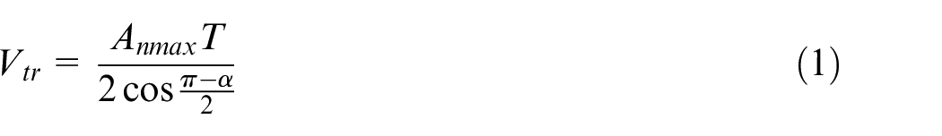
Direct transition.

where $V_{tr}$ represents the maximum speed at the corner, $A_{nmax}$ represents the maximum allowable corner acceleration, T is the interpolation period, $α$ is the Corner Angle (CA).

In equation (1), the maximum allowable corner acceleration and the interpolation period are fixed values. So, when the corner α decreases, the maximum speed at the corner increases.

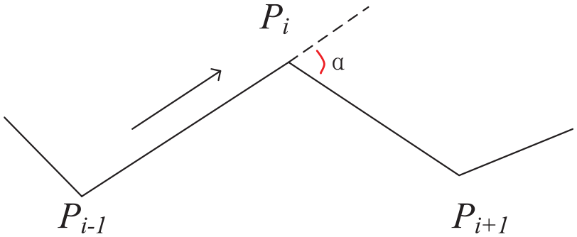
(2)Straight line segment transition. As shown in Figure 2, the straight line segment transition is performed by connecting two transition points on two adjacent line segments by a straight line. This method needs to meet the maximum allowable trajectory error $δ_{\max}$ . In order to ensure the error limit, the length of line segments $P_{i} P_{s}$ , $P_{i} P_{e}$ must meet equation (2).

\bar{P_{i} P_{s}} = \bar{P_{i} P_{e}} \leq \frac{δ_{\max}}{\cos (\frac{π - α}{2})}

(2)

Figure 2.

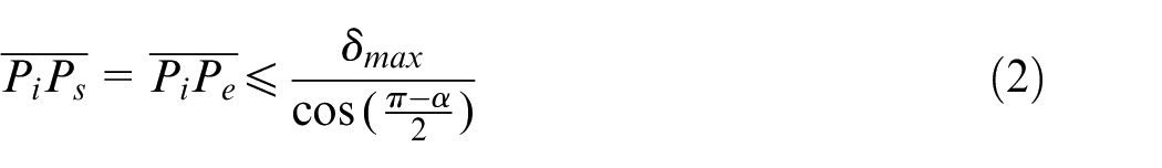
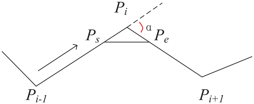
Straight line segment transition.

where $δ_{\max}$ is the maximum allowable trajectory error, $\bar{P_{i} P_{s}}$ is the length of line segment $P_{i} P_{s}$ , $\bar{P_{i} P_{e}}$ is the length of line segment $P_{i} P_{e}$ .

At the same time, in order to ensure that the next line segment has enough transfer length, the length of line segments $P_{i} P_{s}$ , $P_{i} P_{e}$ must meet equation (3).

\bar{P_{i} P_{s}} = \bar{P_{i} P_{e}} \leq min (\bar{P_{i} P_{i - 1}} / 2, \bar{P_{i} P_{i + 1}} / 2)

(3)

The corner speed must satisfy equation (4):

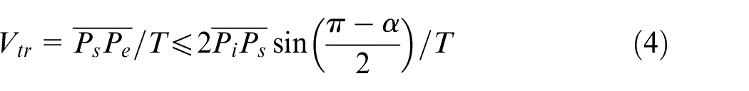
V_{tr} = \bar{P_{s} P_{e}} / T \leq 2 \bar{P_{i} P_{s}} \sin (\frac{π - α}{2}) / T

(4)

In order to meet the maximum corner acceleration limit of the machine tool, it is necessary to meet equation (5):

V_{tr} \leq A_{nmax} T / (2 \cos ((2 π - α) / 4))

(5)

According to equations (4) and (5), equation (6) can be obtained:

\begin{matrix} V_{tr} = min {2 \bar{P_{i} P_{s}} \sin ((π - α) / 2) / T, A_{nmax} T / \\ (2 \cos ((2 π - α) / 4))} \end{matrix}

(6)

According to equation (6), when the CA α decreases, the speed value at the corner increase; at the same time, according to equation (3), when the Length of the Line Segment (LLS) increases, the LLS $P_{i} P_{s}$ increase too, and accordingly the speed value at the corner increase.

(3)Arc transition. The arc transition is the most common transition method. As shown in Figure 3, the maximum allowable trajectory error $δ_{\max}$ also needs to be met. If the short line segment is long enough, the arc radius is expressed as equation (7).

R = \frac{δ_{\max} \sin ((π - α) / 2)}{2 (1 - \sin ((π - α) / 2))}

(7)

Figure 3.

Arc transition.

where R is the arc radius.

At the same time, the line segments $P_{i} P_{s}$ ; $P_{i} P_{e}$ need to meet equation (8).

\bar{P_{i} P_{s}} = \bar{P_{i} P_{e}} \leq min (\bar{P_{i} P_{i - 1}} / 2, \bar{P_{i} P_{i + 1}} / 2)

(8)

If the short line segment is not long enough, the arc radius R is as equation (9).

\begin{matrix} R = min {\bar{P_{i} P_{i - 1}} \tan ((π - α) / 2) / 2, \\ \bar{P_{i} P_{i + 1}} \tan ((π - α) / 2) / 2} \end{matrix}

(9)

Then equation (10) can be obtained when the maximum corner acceleration of the machine tool is met.

V_{tr} \leq \sqrt{A_{nmax} R}

(10)

When the chord height does not exceed the maximum limit value, equation (11) can be obtained.

V_{tr} \leq \frac{2}{T} \sqrt{δ_{\max} R - \frac{{δ_{\max}}^{2}}{4}} \approx \frac{2}{T} \sqrt{δ_{\max} R}

(11)

Since it is necessary to ensure that there are at least two interpolation points on the arc, equation (12) is obtained:

{\begin{matrix} \frac{L_{c}}{V_{tr} T} = \frac{R θ}{V_{tr} T} \geq 1 \\ V_{tr} \leq R θ / T \end{matrix}

(12)

Thus, the corner speed takes the minimum value of equations (10)–(12), as in equation (13):

V_{tr} = min {\sqrt{A_{nmax} R}, \frac{2}{T} \sqrt{δ_{\max} R}, R θ / T}

(13)

From equation (13), when the CA α decreases, R increases, so the speed at the corner increases; when the LLS increases, R increases, and consequently, the speed at the corner increases.

(4)Spline transition. The spline transition is a more advanced transition method in CNC system. The calculation spline transition is more complicated, including Ferguson spline, Bezier spline, NURBS spline, and PH spline. This method is similar to the arc transition, which is related to the maximum curvature of the transition curve. Its curvature and corner speed are calculated as equations (14) and (15).

ρ = \frac{8 \cos ((π - α) / 2)}{3 d \sin^{2} ((π - α) / 2)}

(14)

V_{tr} = min {\sqrt{\frac{A_{nmax}}{ρ}}, \sqrt{\frac{8 δ}{ρ}} / T}

(15)

where $ρ$ is curvature, d is the length of $P_{i} P_{s}$ .

It can be seen from equations (14) and (15) that when the CA α decreases, $ρ$ decreases, and consequently the speed value at the corner increases. Similar to the arc transition, the increased LLS increases the transition space, which increases the corner speed as well.

To sum up, no matter which corner transition method is used, a relatively small CA and a relatively large LLS help to increase the speed at the corner. Based on the above analysis, the objective function to recalculate the CL point is constructed in Section 3 based on the LLS and CA to improve the speed at the corner.

Construction of objective function and calculation method of CL points

According to the analysis results in Section 2, increasing the LLS of the tool path as much as possible and reducing the CA of the adjacent short line segment can increase the speed at the corner. However, since the LLS and the CA are related to each other, when the LLS increases, the CA will increase; conversely, when the LLS decreases, the CA will decrease. Thus, increasing the LLS of the tool path and reducing the CA of the adjacent short line segment are contradictory. This section reconciles the two contradictions to achieve the goal of increasing the LLS and reducing the CA of the adjacent short line segment. On this basis, the calculation method of the CL points will be established.

Construction of objective function

According to the above analysis, the following conditions need to be satisfied for the objective function construction. (1) When CA is as small as possible and LLS is as large as possible, the corner speed can be increased. (2) CA and LLS are in contradiction. Therefore, the equations are constructed to reconcile the two contradictions.

To achieve the reconciliation of the two contradictory goals, the following objective function is proposed as shown in equation (16).

max f (l, α) = a \frac{l}{\bar{L}} + b \frac{\bar{α}}{α}

(16)

where $\bar{L}$ is the average LLS in the case of equal-chord height dispersion, $\bar{α}$ is the average CA in the case of equal-chord height dispersion, and a and b are defined as the weight coefficients of the LLS and the CA, respectively, a + b = 1.

The length l of the line segment connecting the adjacent CL points is used as the numerator of the first term on the right side of the equation, and the CA α of the adjacent short line segment is used the denominator of the second term on the right side. When l increases, the left side of the equation increases; as α decreases, the left side of the equation also increases. It can be seen from equation (16) that when $f (l, α)$ takes the maximum value, the LLS can be as large as possible and the CA of the adjacent short line segment as small as possible at the same time. By equation (16), the reconciliation of the two contradictory goals can be achieved. Meanwhile, the local optimal CL points can be obtained.

Calculation method of CL points

The CAD/CAM system uses NURBS parametric curves to express the sculptured surface parts. The ISO uses NURBS as the only mathematical method for defining the geometry of industrial products. Similarly, the curve obtained in CAM system from the CAD system is a NURBS curve. Based on this, the calculated curves in the following process are all NURBS curves.

Since the calculation of the CL points needs to meet the constraint of the chord height, the calculation method of the chord height of the NURBS curve is established in this section. This method will be used in the subsequent solution process of the CL points. A k-th degree NURBS curve is defined as equation (17).

P (u) = \frac{\sum_{i = 1}^{n} ω_{i} d_{i} N_{i, k} (u)}{\sum_{i = 1}^{n} ω_{i} N_{i, k} (u)}

(17)

where

{\begin{matrix} N_{i, 0} (u) = {\begin{matrix} 1, & (t_{i} \leq u \leq t_{i + 1}) \\ 0, & (o t h e r s) \end{matrix} \\ \begin{matrix} N_{i, k} (u) = \frac{(u - t_{i}) N_{i, k - 1} (u)}{t_{i + k} - t_{i}} + \frac{(t_{i + k - 1} - u) N_{i + 1, k - 1} (u)}{t_{i + k + 1} - t_{i + 1}}, k \geq 1 \\ D E F I N E i f d e n o m i n a t o r = 0, e q u a t i o n = 0 \end{matrix} \end{matrix}

where d_i is the control point, ω_i is the weight, k is the degree of the NURBS curve, and N_i,k(u) is the k-order B-spline basis function calculated from the knot vector U = [u₀, u₁,…u_n_{+ k + 1}].

A NURBS curve is uniquely determined by its control points, the corresponding weights, and the knot vector.

Figure 4 shows the chord height of the NURBS curve, which is solved as equation (18).

\begin{matrix} E = r - \sqrt{r^{2} - {(\frac{L}{2})}^{2}} \approx \frac{θ^{2} \times r}{2} \\ θ \approx \frac{L}{2 r} \\ \Rightarrow E \approx \frac{L^{2}}{8 r} \end{matrix}

(18)

Figure 4.

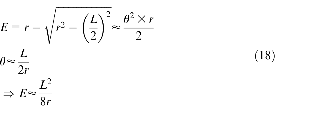
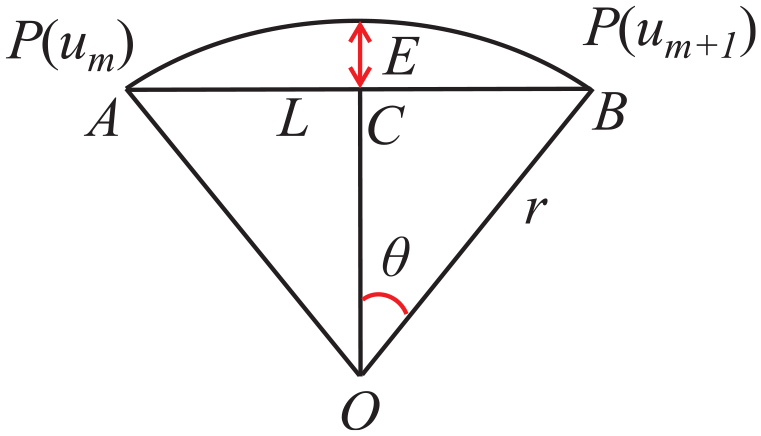
Chord height of the NURBS curve.

where E is chord height, L is the chord length of AB, θ is $∠ BOC$ , and r is the radius of curvature.

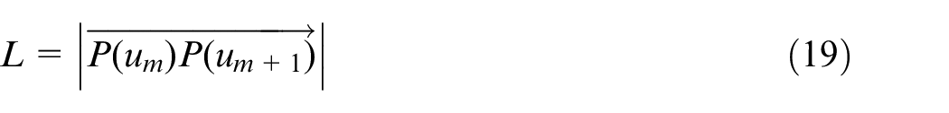
It can be seen from equation (18) that E can be solved by solving L and r. In Figure 4, points A and B are points on the NURBS curve, so point A is represented as $P (u_{m})$ , point B is represented as $P (u_{m + 1})$ , and thereby the solution of L is as equation (19).

L = | \vec{P (u_{m}) P (u_{m + 1})} |

(19)

And the solution of r is as equation (20).

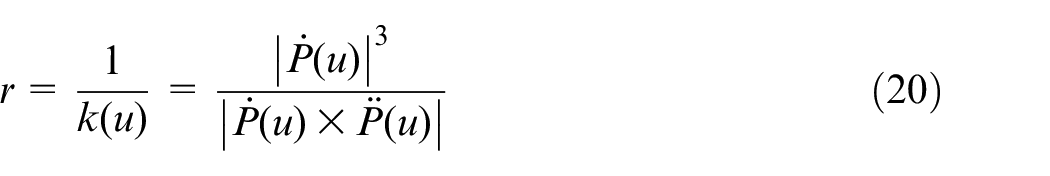
r = \frac{1}{k (u)} = \frac{{| \overset{\cdot}{P} (u) |}^{3}}{| \overset{\cdot}{P} (u) \times \overset{\cdot\cdot}{P} (u) |}

(20)

where $k (u)$ is the curvature of the curve, $\overset{\cdot}{P} (u)$ is the first derivative of the curve, and $\overset{\cdot\cdot}{P} (u)$ is the second derivative of the curve.

Let $A (u) = \sum_{i = 1}^{n} ω_{i} d_{i} N_{i, k} (u)$ , $B (u) = \sum_{i = 1}^{n} ω_{i} N_{i, k} (u)$ , then equation (17) can be written as equation (21).

P (u) = \frac{A (u)}{B (u)}

(21)

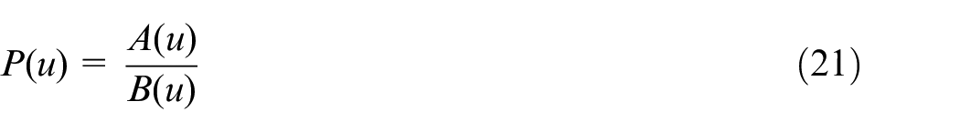
The first and second derivatives of the NURBS curve can be obtained according to equations (22) and (23).

\overset{\cdot}{P} (u) = \frac{\overset{\cdot}{A} (u) B (u) - A (u) \overset{\cdot}{B} (u)}{B^{2} (u)} = \frac{1}{B (u)} (\overset{\cdot}{A} (u) - P (u) \overset{\cdot}{B} (u))

(22)

\overset{\cdot\cdot}{P} (u) = \frac{\overset{\cdot}{A} (u)}{B (u)} - \frac{P (u) \overset{\cdot}{B} (u)}{B (u)} = \frac{\overset{\cdot\cdot}{A} (u)}{B (u)} - \frac{P (u) \overset{\cdot\cdot}{B} (u)}{B (u)} - 2 \frac{\overset{\cdot}{P} (u) \overset{\cdot}{B} (u)}{B (u)}

(23)

The radius of curvature r can be obtained by substituting equations (22) and (23) into equation (20).

Then the solution procedure of the CL points is as follows:

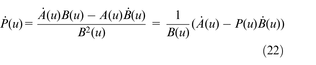
(1)Determination of the chord height E and the first CL point. The chord height E depends on the machining accuracy. As shown in Figure 5, the starting point of the curve is taken as the first CL point.

(2)Solution of the second CL point. As shown in Figure 5(a), the solution of the second CL point needs to consider the constraint of the chord height E. The solution method of the second point is as follows:

Figure 5.

Solution of CL points: (a) Solution of the secondCL point; (b) Solution of the remaining CL points.

According to equation (17), the second CL point can be obtained by solving the knot vector of the second point. Assuming that the knot vector of the first point Us = 0 and the knot vector of the second point Ue = 1, bringing Ue = 1 into equation (17), the chord height e at this time can be solved according to equation (18). If the chord height e is less than or equal to E, Ue will be output; if e is greater than E, Ue = (Us + Ue)/2, the previous process will be repeated until e is less than or equal to E. Then bringing the obtained knot vector into equation (17), the corresponding second CL point can be got.

(3)The solution of the remaining CL points. Taking the solution of the third point as an example, from this point, the solution of the CL points must not only meet the constraint of the chord height E, but also ensure that the LLS is as long as possible and the CA is as small as possible. Figure 5 shows the schematic diagram of the solution from the third CL point to the last one.

Firstly, the feasible region of the third CL point is determined as the green region in Figure 5(b). The range of this feasible region is equation (24):

L_{i} \in [L_{\min}, L_{\max}]

(24)

where $L_{i}$ is the length of the ith short line segment; $L_{\max}$ is the LLS when the chord height e = E; $L_{\min}$ is the LLS when the chord height error e = tE in which t is an adjustable parameter, usually 0.5 < t < 1, t is taken as 0.8 in this study.

It can be seen from the above procedure that the third CL point is a certain point on the curve in the green region in Figure 5(b). By the above objective equation (16), the optimal position of this point in the feasible region will be solved. Each CL point in the feasible region corresponds to a group of l and α. Through bringing each group of l and α into equation (16) respectively, the value of $f (l, α)$ can be solved. The point with the largest $f (l, α)$ value is the third CL point to be solved.

In the same way, the calculation method of the remaining CL points is the same as this point. Until the end point of the curve is reached, the solution of the CL points is completed. The flow chart of the CL point calculation is shown in Figure 6.

Figure 6.

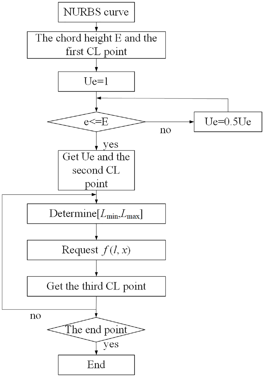
Flow chart of CL points calculation.

Generation of finishing CL points of lower baseline of S-shaped edge strip

The S-shaped piece (ISO10791-7) is a standard piece used to test high-end CNC machine tools. The lower baseline is a flat curve, usually machined by both XY axes, with a distinct curvature variation characteristic. Its S-shaped edge strip has the characteristics of variable curvature. In engineering practice, the G-code of S specimen is in the form of continuous small linear segments, and the interpolation process requires a large number of transitions for the linear segments. Therefore, the lower baseline of the S-shaped edge strip was selected as the experimental verification object.

According to the ISO standard, the lower baseline curve of the S-shaped edge strip was established using the NURBS curve. Based on the NURBS curve, the CL points are generated by both the traditional iso-chord height method and the proposed method for comparison. In the following sections, the CL points generated by the traditional iso-chord height method and the proposed method are called CL points 1 and CL points 2, respectively. The maximum chord height of both CL points 1 and CL points 2 was limited to 0.01 mm. The CL points 1 and the CL points 2 are shown in Figure 7. It shows that the CL points generated by both methods do not deviate from the trajectory, but present obvious differences at some positions.

Figure 7.

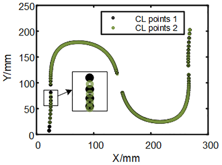
CL points generated by the two method.

The LLS and CA of the CL points generated by the two methods are shown in Figure 8(a) and (b). Among them, the LLS of CL points 2 is smaller than that of CL points 1 where the trajectory curvature is large, and the overall corner of CL points 2 is smaller than that of CL points 1. The results show that the LLS and CA of the CL points generated by the proposed method have changed compared with the iso-chord height method. This is the result after considering the CNC corner transition speed.

Figure 8.

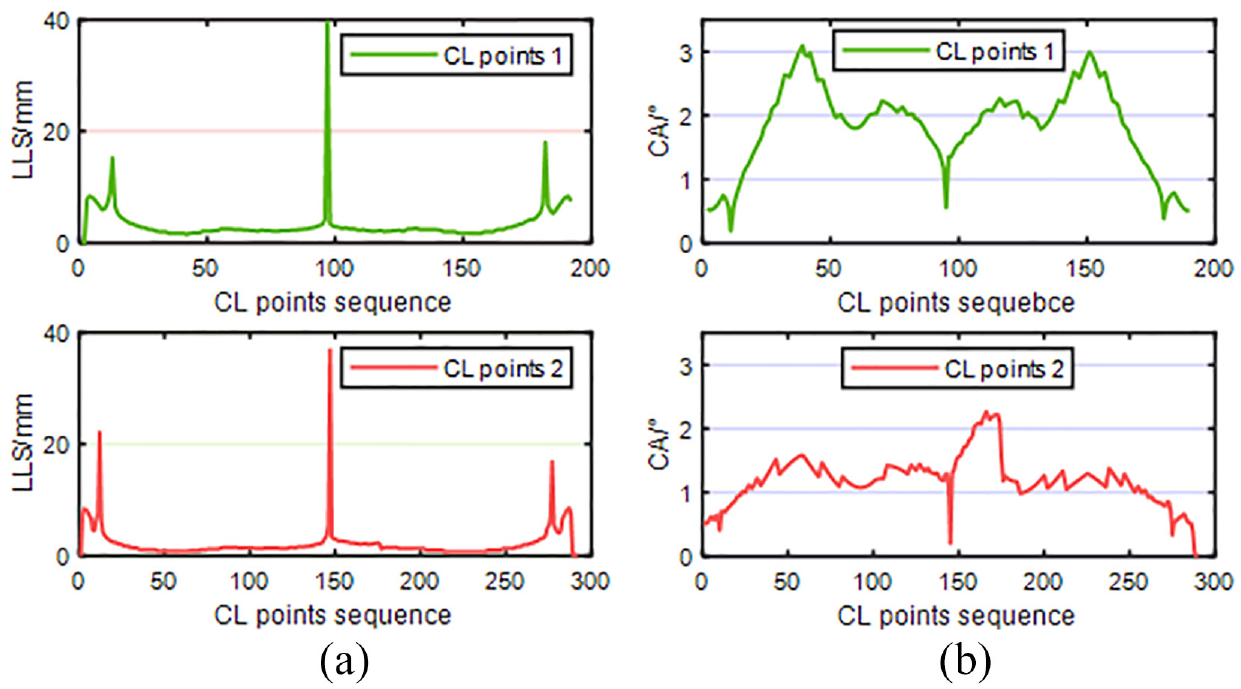
Comparison of the LLS and CA: (a) Comparison of the LLS ; (b) Comparison of the CA.

Experimental testing of S-shaped edge strip motion parameters

The KMC400 U five-axis vertical milling machining center equipped with the GNC62 CNC system was employed for experimental verification. According to the GNC62 CNC system format, the CL points data were converted into the NC codes.

The two NC code files were entered into the GNC62 CNC system, using the G40 code to turn off the tool compensation function, with the S-curve Acceleration and Deceleration control on CNC system. By running the machine tool, the interpolation setpoints and linear encoder data can be collected by the command G237 A3 D576 C2 and G238 in NC code. G237 indicates the start of data collection, A3 means that the data of the X and Y axes are collected, D576 indicates that the data to be collected is the Setpoints Position (SP) and Linear Encoder Feedback Position (LEFP), C2 means that the sampling period is 2 ms, and G238 indicates the end of data collection.

The relationship between the X-axis arc length and setpoints speed of CL points 1 and 2 can be obtained by processing the collected interpolation setpoints data, as shown in Figure 9(a). The experimental feed rate was set to 5000 mm/min. It can be seen from the figure that the setpoints speed curve of CL points 2 is smoother than that of CL points 1. In the arc lengths of 140 to 190 mm and 440 to 490 mm, the setpoints speed of CL points 2 increases significantly, and the curve fluctuation decreases. According to the relationship between cutting force and speed, faster speed will inevitably cause an increase in cutting force.

Figure 9.

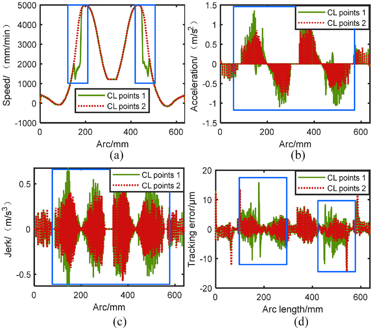
Comparison of setpoints speed, acceleration, jerk, and tracking error: (a) Comparison of setpoints speed;(b) Comparison of setpoints acceleration; (c) Comparison of setpoints jerk; (d) Comparison of setpoints tracking error.

Figure 9(b) shows the comparison of the X-axis setpoints acceleration of CL points 1 and CL points 2. It can be seen from this figure that the acceleration of CL points 2 decreases in the area where the speed increases. Likewise, Figure 9(c) shows the setpoints jerk of CL points 1 and CL points 2. It can be seen from this figure that the jerk is also reduced in the same area. Acceleration and acceleration become smaller, and the vibration generated by the machine will be reduced accordingly.

The tracking error can be obtained through the collected LEFP data and SP data. Figure 9(d) shows the comparison of the tracking errors of the X-axis of CL points 1 and CL points 2. It can be seen from the figure that the method proposed can significantly reduce the tracking error overall. In the blue box of the figure, the tracking error of CL points 2 can be reduced by 4–12 μm compared to CL points 1.

Figure 10 compares the trajectory at SP and LEFP. The tracking errors of the X and Y axis are magnified by a factor of 500 for better observation of the difference between the trajectories. It can be found that the deviation between the trajectory at SP and the trajectory at LEFP of CL points 2 is significantly smaller than that of CL points 1. In addition, the trajectory at LEFP of CL points 2 is smoother compared with that of CL points 1. It means that the method proposed can facilitate the reduction the trajectory deviation and suppression of the vibration during machining.

Figure 10.

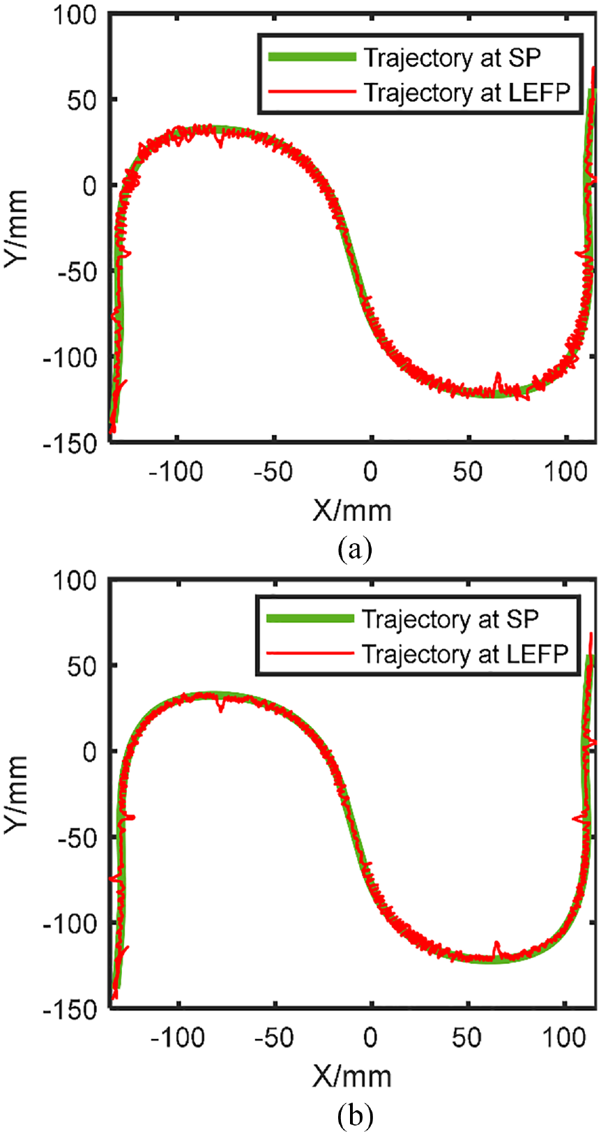
Comparison of trajectory at SP and the trajectory at LEFP. (a) CL points 1 and (b) CL points 1.

The frequency domain information of the data collected by linear encoder can be obtained through the FFT. Figure 11 shows the frequency spectrum of LEFP during the processing of CL points 1 and CL points 2. It can be seen from the figure that the vibration is obviously weakened when the CL points are generated by the proposed method, which helps to improve the machining accuracy.

Figure 11.

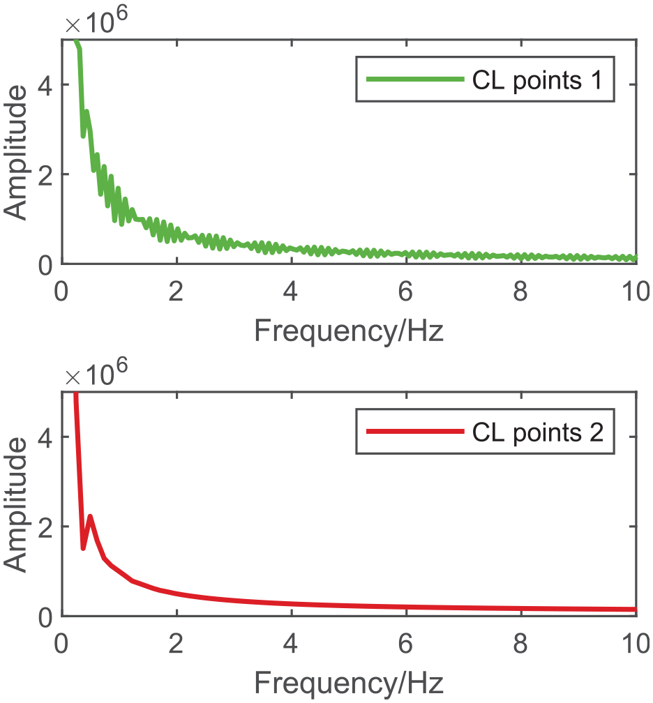
Frequency spectrum of LEFP.

Moreover, the machining time of CL points 1 and CL points 2 are calculated for comparison of the machining efficiency. The machining time of CL points 1 is 8.748 s, while that of CL points 2 is 8.162 s. The machining time of CL points 2 is 7.18% less than that of CL points 1.

Conclusions

For the CL points used for continuous small linear interpolation methods, the Calculation Method of Cutter Location Points Considering Corner Transition Speed in CNC is proposed, and the conclusions are as follows:

A calculation method of CL points considering the transition speed of the corner transition algorithm in CNC is proposed. This method can generate more optimal CL points.

The proposed CL points calculation method can increase the setpoints speed at the corner, while reducing the setpoints acceleration and jerk. Furthermore, by the proposed method, the tracking accuracy, trajectory accuracy, and machining efficiency can be significantly improved. Taking the S-shaped trajectory as an example, the CL points generated by the proposed method make the tracking error reduce by 4–12 μm, and make the machining efficiency improve by 7.18%.

Footnotes

Declaration of conflicting interests

The author(s) declared no potential conflicts of interest with respect to the research, authorship, and/or publication of this article.

Funding

The author(s) disclosed receipt of the following financial support for the research, authorship, and/or publication of this article: This work is financially supported by the project of National Natural Science Funds of China (Grant No. 52175483).

ORCID iDs

Dun Lyu

Yanhong Song

References

Lyu

Liu

, et al. Dynamic error of CNC machine tools: a state-of-the-art review. Int J Adv Manuf Technol 2020; 106: 1869–1891.

Chen

Kang

Wang

, et al. Tool path optimal design for slow tool servo turning of complex optical surface. Proc IMechE, Part B: J Engineering Manufacture 2017; 231: 825–837.

Yao

Sang

, et al. Tool path regeneration in five-axis flank milling for ruled surface based on error distribution. Proc IMechE, Part B: J Engineering Manufacture 2022; 236: 1751–1759.

Bobrow

. NC machine tool path generation from CSG part representations. Comput Des 1985; 17: 69–76.

Elber

Cohen

. Toolpath generation for freeform surface models. Comput Des 1994; 26: 490–496.

Erkorkmaz

Altintas

. High speed CNC system design. Part III: high speed tracking and contouring control of feed drives. Int J Mach Tools Manuf 2001; 41: 1637–1658.

. CNC machine tool surface interpolator for ball-end milling of free-form surfaces. Int J Mach Tools Manuf 2000; 40: 307–326.

Loney

Ozsoy

. NC machining of free form surfaces. Comput Des 1987; 19: 85–90.

Min

Gao

. Iso-scallop tool-path generation of five-axis computer numerically controlled machining for cyclide splines. Proc IMechE, Part B: J Engineering Manufacture 2015; 229: 1144–1156.

10.

Huang

Oliver

. Non-constant parameter NC tool path generation on sculptured surfaces. Int J Adv Manuf Technol 1994; 9: 281–290.

11.

Lartigue

Thiebaut

Maekawa

. CNC tool path in terms of B-spline curves. Comput Des 2001; 33: 307–319.

12.

Park

Choi

. Tool-path planning for direction-parallel area milling. Comput Des 2000; 32: 17–25.

13.

Sarma

. The crossing function and its application to zig-zag tool paths. Comput Des 1999; 31: 881–890.

14.

Lee

. Non-isoparametric tool path planning by machining strip evaluation for 5-axis sculptured surface machining. Comput Des 1998; 30: 559–570.

15.

. Efficient cutter-path planning for five-axis surface machining with a flat-end cutter. Comput Des 1999; 31: 557–566.

16.

Suresh

Yang

DCH

. Constant scallop-height machining of free-form surfaces. J Eng Ind 1994; 116: 253–259.

17.

Zhang

Nee

AYC

Fuh

JYH

. An efficient cutter contact curve tool path regeneration algorithm for sculptured surface machining. Proc IMechE, Part B: J Engineering Manufacture 2004; 218: 389–402.

18.

Marciniak

. Influence of surface shape on admissible tool positions in 5-axis face milling. Comput Des 1987; 19: 233–236.

19.

Kruth

Klewais

. Optimization and dynamic adaptation of the cutter inclination during five-axis milling of sculptured surfaces. CIRP Ann 1994; 43: 443–448.

20.

Kim

Sarma

. Toolpath generation along directions of maximum kinematic performance; a first cut at machine-optimal paths. Comput Des 2002; 34: 453–468.

21.

Chiou

Lee

. A machining potential field approach to tool path generation for multi-axis sculptured surface machining. Comput Des 2002; 34: 357–371.

22.

Giri

Bezbaruah

Bubna

, et al. Selection of master cutter paths in sculptured surface machining by employing curvature principle. Int J Mach Tools Manuf 2005; 45: 1202–1209.

23.

Meng Lim

Menq

. Integrated planning for precision machining of complex surfaces. Part 1: cutting-path and feedrate optimization. Int J Mach Tools Manuf 1997; 37: 61–75.

24.

Liu

Zhao

, et al. Tool path generation for turbine blades machining with twin tool. J Manuf Sci Eng 2017; 139: 111015.

25.

Liu

, et al. Optimal cutting directions by considering the dynamic mismatch between feed axes of machine tools. Int J Adv Manuf Technol 2018; 95: 1607–1615.

26.

Zhong

Luo

Chang

, et al. Toolpath interpolation and smoothing for computer numerical control machining of Freeform surfaces: a review. Int J Autom Comput 2020; 17: 1–16.

27.

Fan

Lee

Chen

. A realtime curvature-smooth interpolation scheme and motion planning for CNC machining of short line segments. Int J Mach Tools Manuf 2015; 96: 27–46.

28.

Zhao

Zhu

, et al. Look-ahead interpolation of short line segments using B-spline curve fitting of dominant points. Proc IMechE, Part B: J Engineering Manufacture 2015; 229: 1131–1143.

29.

Yuen

Zhang

Altintas

. Smooth trajectory generation for five-axis machine tools. Int J Mach Tools Manuf 2013; 71: 11–19.

30.

Wang

Yang

Liu

. A real-time look-ahead interpolation algorithm based on Akima curve fitting. Int J Mach Tools Manuf 2014; 85: 122–130.

31.

Shi

Wang

, et al. Analytical curvature-continuous dual-Bézier corner transition for five-axis linear tool path. Int J Mach Tools Manuf 2015; 91: 96–108.

32.

Shi

Zhu

, et al. Corner rounding of linear five-axis tool path by dual PH curves blending. Int J Mach Tools Manuf 2015; 88: 223–236.

33.

Tulsyan

Altintas

. Local toolpath smoothing for five-axis machine tools. Int J Mach Tools Manuf 2015; 96: 15–26.

34.

Huang

Zhu

. Real-time local smoothing for five-axis linear toolpath considering smoothing error constraints. Int J Mach Tools Manuf 2018; 124: 67–79.

35.

Lin

Lee

Shen

, et al. Local corner smoothing with kinematic and real-time constraints for five-axis linear tool path. In: 2018 IEEE/ASME international conference on advanced intelligent mechatronics (AIM), 2018. New York: IEEE.

Calculation method of cutter location points considering corner transition speed in CNC

Abstract

Keywords

Introduction

Key geometric parameters of CL points affecting corner speed

Construction of objective function and calculation method of CL points

Construction of objective function

Calculation method of CL points

Generation of finishing CL points of lower baseline of S-shaped edge strip

Experimental testing of S-shaped edge strip motion parameters

Conclusions

Footnotes

Declaration of conflicting interests

Funding

ORCID iDs

References