Sage Journals: Discover world-class research

Abstract

Axial-flow pumps with siphon outlet are widely used in South-to-North Water Transfer Project of China for the excellent characteristics and good performance in stopping period. The reverse rotational speed and the head of impeller are the key parameters for the system’s safety in stoppage. In this article, the computational fluid dynamics method was used for three-dimensional unsteady numerical simulations. The method based on volume of fluid model was executed on geometrical model of the whole flow system to get the variation laws of internal and external characteristic parameters. Through numerical calculation, the variation laws of the parameters were got in the pump operating condition, braking condition, and turbine condition, and the maximum reverse speed of the impeller was 203.0 r/min (−0.947 times the rated speed). Compared with the designed mode, when the air valve was opened in advance, the pump system would go through the weir flow state first, and a higher head of impeller would be got as a result. When the air valve refused to open, the pump system would get into runaway state. Comparisons of the calculated and measured results indicate the proposed computational fluid dynamics method is reliable in the simulation of the transient flow in axial-flow pump system.

Keywords

Numerical simulation axial-flow pump stoppage siphon outlet volume of fluid model

Introduction

Axial-flow pumps are widely used in the water transfer project, agricultural irrigation, and urban water supply for the advantage of large flow, low head. The axial-flow pump with a siphon outlet is commonly used. The air valve on the top of siphon outlet is used to export air in unit startup and to import air in stopping process. By opening the air valve to import air, the pump system can get the quick and reliable cut-off of water in stopping process.¹ However, the siphon outlet has a higher geometry elevation on the top, and it leads to larger backflow and reverse rotational speed. So, it is very important to get the variation laws of internal and external characteristics in stopping process in engineering application.²

During the past few decades, there have been several studies on the transient characteristics of turbo-machine systems.³ Tanaka and Tsukamoto⁴ explored the transient phenomena at pump startup/shutdown processes of a centrifugal pump. A Dazin et al.⁵ used angular momentum equations and energy equations to predict the torque, power, and head of the impeller under transient operating conditions. The transient flow through a centrifugal pump during startup process with the method of characteristics (MOC) was researched by C Issa et al.⁶

Nowadays, computational fluid dynamics (CFD) method is increasingly used to capture complex three-dimensional (3D) features inside the fluid machinery.^7,8 Dedicated experiments for the validation of CFD codes applied in pump have already been performed by W-d Shi et al.⁹ J Feng et al.¹⁰ got the influence of the tip clearance in axial-flow pump using CFD method. The performance of axial-flow pump with adjustable guide vane was simulated by Z-d Qian et al.¹¹ These studies enable us to improve our understanding of the flow characteristics in pump systems.

Although accurate and efficient simulation of unsteady flow phenomena remains one of the main challenges for CFD in turbo-machine systems, some achievements were made by comparing with experiments.¹² M Fortin et al.¹³ used unsteady methods to simulate the flow within a turbine model in runaway condition. D Zhou et al.¹⁴ simulated the runaway of axial-flow pump system caused from power failure using unsteady CFD method. Various numerical setups for modeling Francis turbine startups were presented by J Nicolle et al.¹⁵ Z Li et al.¹⁶ investigated the transient characteristics in a centrifugal pump during startup process experimentally and numerically. The transient behaviors of the centrifugal pump in stopping process were simulated by Y-l Zhang et al.¹⁷

In this article, the volume of fluid (VOF) multiphase flow model and the dynamic mesh of the FLUENT code¹⁸ were used to simulate the stopping process in axial-flow pump system. Cases of air valve opened in advance or refusing to open were simulated in addition to the designed mode (air valve opened with the motor’s power-off at the same time). The parameters were got from the simulations such as maximum reverse speed and maximum head of impeller.

Numerical methodology

Geometry

Figure 1 shows the geometric model of a vertical axial-flow pump driven directly by the motor, and the designed stopping mode is the air valve opening with the motor’s power-off at the same time. The ratio of the model pump and the prototype pump is 1:1, and the suction sump, the elbow inlet passage, the impeller, the guide vane, the siphon outlet passage, the outlet sump, and other components are included. The mounting angle of the blades is 0°, and the other parameters of the axial-flow pump are showed in Table 1.

Figure 1.

Geometrical model of axial-flow pump system.

Table 1.

Parameters of axial-flow pump system.

Parameter	Symbol	Value
Rated head of system	H_R (m)	2.75
Rated discharge	Q_R (m³/s)	11.5
Rated rotational speed	N_R (r/min)	214.3
Rotary inertia	J (kg m)	2800
Diameter of impeller	D (mm)	1750
Number of impeller blades	Z	4
Number of guide vanes	Z_g	5
Elevation of impeller	H ₀ (m)	−3.5
Elevation of air valve	H ₁ (m)	9.2
Elevation of suction sump	H ₂ (m)	0.8
Elevation of outlet sump	H ₃ (m)	3.55

Grid generation and boundary conditions

The Gambit meshing software was used to generate the unstructured grids for the whole model. The grids in the zones of impeller and guide vane were refined for the complex flow. It could be found from Table 2 that the number of cells had little effect when it was large enough, and the head and discharge in scheme 3 had little difference to the rated values. So as to improve the computational efficiency, scheme 3 was chose to mesh the model, and the number of cells was 2.45 million.

Table 2.

Tests of different meshing schemes.

Scheme	Mesh number (105)							Head (m)	Discharge (m³/s)
	Suction sump	Inlet	Impeller	Guide vane	Outlet	Outlet sump	Total
1	3.1	2.0	3.0	2.7	2.8	2.4	16.0	2.60	11.31
2	3.1	2.8	3.8	3.9	4.1	2.4	20.1	2.68	11.41
3	3.1	3.7	5.0	5.2	5.1	2.4	24.5	2.74	11.48
4	3.1	4.6	6.2	6.4	6.0	2.4	28.7	2.76	11.51

The boundary conditions were set as follows: the pressure-inlet boundary condition was set at the inlet of the suction sump and the air tank, and the relative total pressure, turbulent kinetic energy, and its diffusion rate were given; the pressure-outlet boundary condition was set at the outlet of the outlet sump, and the relative static pressure, turbulent kinetic energy, and its diffusion rate were prescribed; the moving mesh model was used to simulate the rotation of the impeller and the air valve, and the interface boundary condition was set at both sides of the air valve; no-slip boundary condition was applied to the wall; and standard wall functions were applied to the region near the wall.

Numerical simulation procedures

The interactive flow of air and water phase in the outlet passage and air valve is an important part of the transient numerical simulations in stopping process. The VOF model has a good performance in tracking the interface between air and water by solving the volume fraction equation;¹⁹ so, the VOF model was used to monitor the variation of gas–liquid two-phase flow. The governing equations of the VOF formulations on multiphase flow are as follows

Equation of continuity

\frac{\partial ρ}{\partial t} + \nabla \cdot (ρ \vec{v}) = 0

(1)

Equation of motion

\frac{\partial (ρ \vec{v})}{\partial t} + \nabla \cdot (ρ \vec{v} \vec{v}) = - \nabla p + \nabla \cdot [μ (\nabla \vec{v} + \nabla {\vec{v}}^{T})] + \vec{F}

(2)

Volume fraction equation

\frac{\partial α_{1}}{\partial t} + \vec{v} \cdot \nabla α_{1} = 0, \frac{\partial α_{2}}{\partial t} + \vec{v} \cdot \nabla α_{2} = 0

(3)

where $α_{1}$ and $α_{2}$ are the volume fraction of water and gas phase, $α_{1} + α_{2} = 1$ ; $\vec{v}$ is the velocity vector; $ρ$ is the density; $μ$ is the dynamic viscosity; $t$ is the time; ∇ is the Hamiltonian; $p$ is the static pressure; and $\vec{F}$ is the surface tension force of the fluid. The bulk properties such as density and viscosity are determined from the volume fraction weighed average of the properties of the two fluids, that is

ρ = α_{1} ρ_{1} + α_{2} ρ_{2}, μ = α_{1} μ_{1} + α_{2} μ_{2}

(4)

where the subscript 1 indicates gas and 2 indicates the liquid phase.

The governing equations were discrete with finite volume method (FVM), and the first-order upwind scheme was used for the convection items with a central difference scheme for the diffusion terms, and the pressure implicit with splitting of operators (PISO) algorithm was adopted to realize the velocity–pressure coupling solution. The realizable k–ε turbulence model²⁰ based on the VOF model was also used with water as the primary phase and gas as the second phase.

Torque balance equation

The user-defined function (UDF) of the FLUENT code was used to control the changing law of the rotational speed of the impeller based on the torque balance equation, that is

M = J \frac{d ω}{dt}

(5)

where M is the total torque of the impeller, J is the rotary inertia, ω is the angular velocity, and $t$ is the time. The mechanical friction torque and the rotor wind resistance torque are not included in the total torque.

Results

After the entrance of air and the loss of active torque on the impeller, the pump system would get into the pump operating condition, braking condition, turbine condition, until the end of the stopping process. The designed stopping mode was simulated as well as the cases of air valve opened in advance or refusing to open.

Analysis on characteristics in designed mode

Figure 2 shows the distribution of air and water phases of the axial-flow pump with siphon outlet during stopping process. The stopping mode was that the air valve was opened with motor’s power-off at the same time. After a 2-s normal operation, air was imported into the outlet quickly as soon as the air valve was opened. An air pocket was formed in the upper part of downward section in the outlet passage because the forward flow still had a large velocity. The flow in the outlet was cut by air at 6 s with the water level of the upward part at the top of siphon, and the water level of the downward part is the same with the outlet sump’s water level. From 6 to 14 s, the water level in the upward part decreased gradually. Then, the downward section’s water level fluctuated in a narrow range and stabilized at the water level of outlet sump finally.

Figure 2.

Distribution of air and water phases.

Figure 3 shows the variation laws of the external characteristic parameters, including the discharge Q, the torque M, the head of impeller H, the static pressure P, the axial force of impeller F, and the rotational speed n. P is the static pressure of the monitoring point which is 0.2 m below the air valve (Figure 1), and the direction of axial force F is upward.

Figure 3.

Variation laws of the external characteristic parameters: (a) Q_in/n–t, (b) Q_in/Q_out–t, (c) H/P–t, and (d) M/F–t.

The pump operating condition was from 2 to 4.97 s. During this time, the inlet flow Q_in decreased rapidly; after air valve’s opening, the water level of the downward part of the outlet passage decreased due to the geometrical characteristics; the outlet flow Q_out increased first and then decreased; the static pressure of monitoring point P increased to atmospheric pressure at the moment of the valve’s opening, and then it returned to vacuum with its value decreasing gradually with sharp fluctuation; the absolute values of the head H, the torque M, the axial force F all had a rapid decline at this stage.

The braking condition was at 4.97–6.31 s. The inlet flow was backward with the outflow, the speed of impeller and the vacuum of measuring point decreased. At this stage, the absolute values of H, M, and F all increased, and the maximum values obtained at 6.31 s were slightly larger than that of normal operation. So, it indicated that the time point 6.31 s is very important in the stopping process.

After 6.31 s, the pump system got into the turbine condition, and the speed was reversed. As it spun up to a high reverse speed, it caused a high resistance to the flow, which developed a high head at the impeller that must be provided for the design. The reverse speed reached the maximum value (203.0 r/min) at 10.64 s which was −0.947 times the rated speed. The other parameters all decreased to 0 gradually in this process until the pump system was completely stopped.

Case of air valve’s advance opening

The stopping modes of the pump system can be distinguished by the sequence of the air valve’s opening and the motor’s power-off, and the designed mode is that the air valve is opened with the motor’s power-off at the same time. There is an important concern when the motor’s power-off is lagging, since the result is not clear. So, the stopping process in this case was simulated, where the air valve was opened at 2 s and the motor lost power at 7 s.

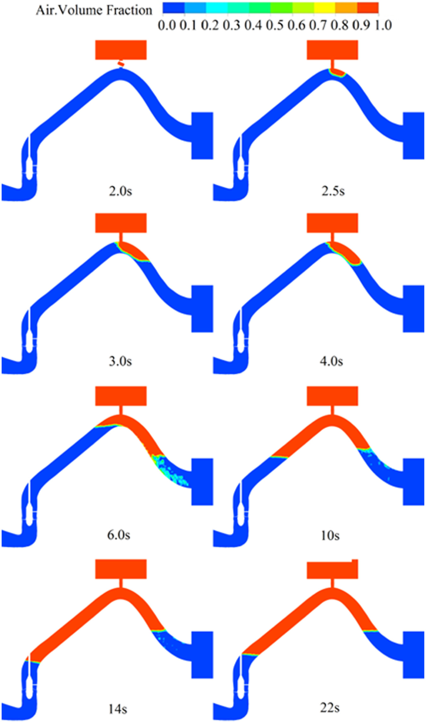
Figure 4 shows the distribution of air and water phases in stopping process with motor’s power-off lagging behind. An air pocket was formed at 4 s in the upper part of downward section in the outlet passage. Compared with which in Figure 2, the air pocket had a lower position because the motor was operating, and the velocity in the outlet passage was large. The weir flow was formed in the outlet passage at 6 s for the motor’s operation, and the temporarily stable state lasted up to 7 s when the motor lost power. The existence of the weir flow is the major difference from the designed mode, and the water level of the upward section will decrease without the motor’s operation. After 7 s, the state of weir flow was destroyed, and the water level of the upward section decreased with the downward section’s water level fluctuating in a narrow range at the water level of the outlet sump.

Figure 4.

Distribution of air and water phases.

Figure 5 is the comparison of rotational speed n, the head of impeller H, the inlet discharge Q_in, and the outlet discharge Q_out in two modes. The maximum reverse rotational speeds in the two modes have little difference, and the two speed curves have a time difference of 5 s. Similarly, the main difference of discharge Q_in and Q_out is the time difference in the two modes. The H-max (maximum of H) of the mode with motor’s power-off lagging was more than 5 m because the pump system got into the state of weir flow prior to the motor’s power-off, and the H-max of the designed mode was only 3.2 m which was much smaller. As a result, the mode with motor’s power-off lagging is not conducive to the safety of pump system.

Figure 5.

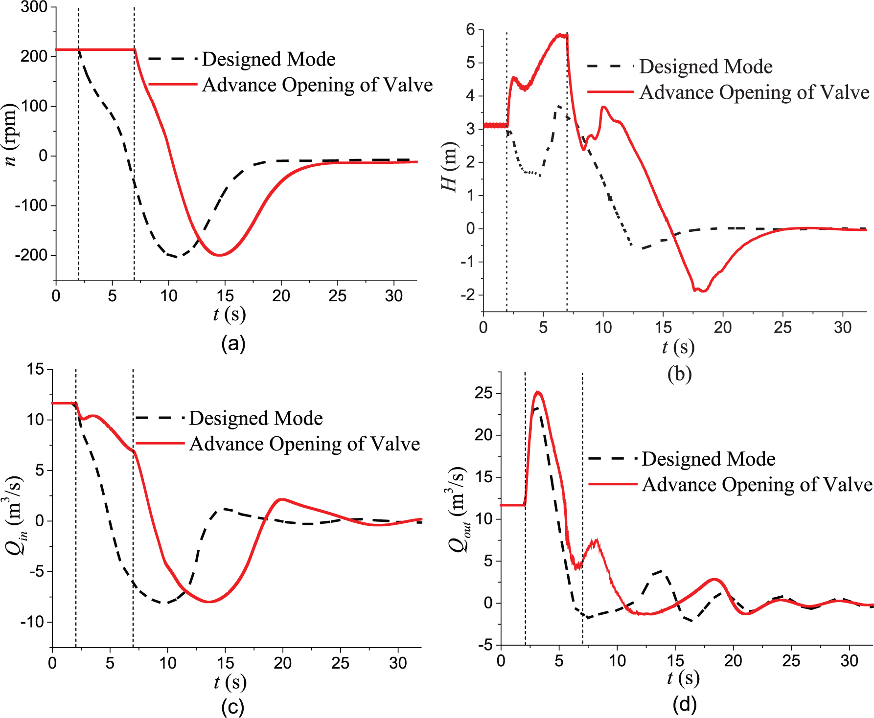
Variation laws of parameters of two modes: (a) n–t, (b) H–t, (c) Q_in–t, and (d) Q_out–t.

From the comparison of the simulation results in the two modes, it can be concluded that the two modes have little difference in the maximums of rotational speed and discharge; however, the mode with motor’s power-off lagging has a larger H-max caused by the weir flow, and it is a disadvantage.

Analysis of runaway

Apparently, if the motor’s power-off is earlier than air valve’s opening, it will lead to larger reflux and reverse rotational speed. Furthermore, the pump system will get into runaway state, if the air valve refuses to open. The runaway speed of the impeller is an important parameter in the stopping process, so the correct value of speed from CFD numerical simulation is necessary.

The CFD numerical simulation was performed under different heads to get the runaway speed. The initial value of rotational speed was 0, and the torque balance equation (5) was used to control the changing law of the rotational speed with UDF. Figure 6 shows the distribution of velocity vectors in runaway state. The direction of the flow was completely reversed, and the static pressure on the top of siphon outlet was negative.

Figure 6.

Velocity vectors in runaway state.

According to the speed law of similarity,²¹ unit runaway rotational speed $n_{11}$ is

n_{11} = \frac{n_{1} D_{1}}{\sqrt{H_{1}}} = \frac{n_{M} D_{M}}{\sqrt{H_{M}}}

(6)

where the subscript 1 indicates the prototype pump, and M indicates the model pump. The unit runaway rotational speed of this pump system is 219.97 r/min based on the model test.²² So, the relationship between $n_{1}$ and $H_{1}$ can be obtained by equation (6) since other parameters are known.

Figure 7 shows that the CFD results agree well with the test results, and the maximum error is less than 5.0%. Compared with test result, the runaway speed is higher in numerical simulation. The difference may be caused by the fact that the radial friction torque on the bearing and the wind drag torque on the rotor are not considered in numerical simulation, and the way using unit speed to obtain runaway speed may be another cause of error. As a whole, the numerical simulation method of the axial-flow pump has high reliability.

Figure 7.

Runaway speeds under different heads.

Conclusion

The stoppage of axial-flow pump system was simulated in this article, and the CFD methods showed high reliability through the comparison of model test and numerical simulation. The following conclusions were obtained:

Through CFD simulations, the pump operating condition, braking condition, and turbine condition could be monitored as well as the parameters.

In the designed mode, the maximum reverse speed of the impeller was −203.0 r/min at 10.64 s, which was −0.947 times the rated speed. The head H, axial force F, and torque M of the impeller reached the maximums at about 6.3 s, and they were larger than the rated values.

In the case of air valve’s advance opening, the pump system would first get into the weir flow state. Compared with designed mode, a higher head of the impeller would be the consequent result which was bad for the safety of the pump system.

Footnotes

Acknowledgements

The support of College of Water Conservancy and Hydropower Engineering, Hohai University, China, is gratefully acknowledged.

Academic Editor: Aditya Sharma

Declaration of conflicting interests

The author(s) declared no potential conflicts of interest with respect to the research, authorship, and/or publication of this article.

Funding

The author(s) disclosed receipt of the following financial support for the research, authorship, and/or publication of this article: The research work was supported by the National Natural Science Foundation of China (grant nos 51079051 and 51339005) and the Priority Academic Program Development of Jiangsu Higher Education Institutions (PAPD).

References

Zhang

Shi

Chen

et al . Unsteady flow analysis and experimental investigation of axial-flow pump. J Hydrodyn 2010; 22: 35–43.

Wang

X-L

Yuan

S-q

Zhu

R-s

et al . Transient hydraulic characteristic study on nuclear reactor coolant pump during stopping period. Atomic Energy Sci Technol 2013; 47: 364–371.

Jiang

Zhai

Wang

et al . Fluid-structure interaction analysis on turbulent annular seals of centrifugal pumps during transient process. Math Probl Eng 2011; 2011: 929574.

Tanaka

Tsukamoto

Transient behavior of a cavitating centrifugal pump at rapid change in operating conditions—part 2: transient phenomena at pump startup/shutdown. J Fluid Eng 1999; 121: 850–856.

Dazin

Caignaert

Bois

Transient behavior of turbomachineries: applications to radial flow pump startups. J Fluid Eng 2007; 129: 1436–1444.

Issa

Elaoud

Akrout

et al . Transient behavior of a centrifugal pump during starting period. Appl Acoust 2016; 109: 82–89.

W-y

Zhang

X-y

Shuai

Z-j

et al . CFD numerical simulation of the complex turbulent flow field in an axial-flow water pump. Adv Mech Eng. Epub ahead of print 12 February 2015. DOI: 10.1155/2014/521706.

Pei

Meng

Y-j

et al . Fluid–structure coupling analysis of deformation and stress in impeller of an axial-flow pump with two-way passage. Adv Mech Eng 2016; 8: 1–11.

Shi

W-d

Zhang

D-s

Guan

et al . Numerical and experimental investigation of high-efficiency axial-flow pump. Chin J Mech Eng 2010; 23: 38–44.

10.

Feng

Luo

Guo

et al . Influence of clearance on pressure fluctuations in an axial flow pump. J Mech Sci Technol 2016; 30: 1603–1610.

11.

Qian

Z-d

Wang

Guo

et al . Performance evaluation of an axial-flow pump with adjustable guide vanes in turbine mode. Renew Energ 2016; 99: 1146–1152.

12.

Song

Numerical simulation of dynamic behavior with rapid-drop gate in vertical axial pumping station during its suspending period. Master Dissertation, Hohai University, Nanjing, China, 2006.

13.

Fortin

Houde

Deschenes

. Validation of simulation strategies for the flow in a model propeller turbine during a runaway event. In: Proceedings of the 27th IAHR symposium on hydraulic machinery and systems, Montreal, QC, Canada, 22–26 September 2014. IOP Conference Series-Earth and Environmental Science 22 (IOP Publishing) 032026.

14.

Zhou

Zhong

Zheng

et al . Numerical simulation of transient flow in axial-flow pump unit model during runaway caused from power failure. J Drain Irrig Mach Eng 2012; 30: 401–406.

15.

Nicolle

Giroux

Morissette

. CFD configurations for hydraulic turbine startup. In: Proceedings of the 27th IAHR symposium on hydraulic machinery and systems, Montreal, QC, Canada, 22–26 September 2014. IOP Conference Series-Earth and Environmental Science 22 (IOP Publishing) 032021.

16.

Peng

Dazhuan

et al . Experimental and numerical study of transient flow in a centrifugal pump during startup. J Mech Sci Technol 2011; 25: 749–757.

17.

Zhang

Y-l

Zhu

Z-c

Cui

B-l

et al . Numerical simulation of unsteady flow in centrifugal pump during stopping period. J Eng Thermophys 2012; 12: 2096–2099.

18.

Fluent (Computer software). Philadelphia, PA: ANSYS, 2014.

19.

Hongtruong

Wen

Zhang

Numerical simulation and analysis of gas-liquid flow in a T-junction microchannel. Adv Mech Eng. Epub ahead of print 26 January 2015. DOI: 10.1155/2012/231675.

20.

Zhao

X-z

C-h

Sun

Z-c.

Numerical simulation of extreme wave generation using VOF method. J Hydrodyn 2010; 4: 466–477.

21.

Wylie

Streeter

VL.

Fluid transients. New York: McGraw-Hill, 1978.

22.

Fei

Dai

et al . Pumping system model tests of datao I pumping station. J Water Res Architect Eng 2013; 11: 126–129.

Transient flow analysis in axial-flow pump system during stoppage

Abstract

Keywords

Introduction

Numerical methodology

Geometry

Grid generation and boundary conditions

Numerical simulation procedures

Torque balance equation

Results

Analysis on characteristics in designed mode

Case of air valve’s advance opening

Analysis of runaway

Conclusion

Footnotes

Acknowledgements

Declaration of conflicting interests

Funding

References