
Abstract
In order to study the effect of solid–liquid two-phase abrasive flow on the surface of inner wall of the special-shaped cavity and relationship between finishing parameters and surface quality, the process of abrasive flow finishing non-linear pipe is numerically simulated. Taking the T tube as the research object, the inlet pressure and outlet pressure change, and abrasive viscosity and other factors were maintained. Then, a test scheme is designed by orthogonal test, which verifies the correctness of the simulation. The T-pipe inner surface roughness is measured, according to the roughness data; the contribution of process parameters to finishing quality is analyzed using Six Sigma Theory. By analyzing the experimental data, optimum technology parameters and regression equation of surface roughness degree with volume fraction, which can be used to guide the abrasive flow actual finishing, are obtained, and it is found that the simulating results are identical with the test results.
Introduction
The surface quality is critical in functional requirements of a job. The traditional finishing processes in the manufacturing of precision parts play an important role, labor intensive and uncontrollable. These finishing techniques are mainly limited to flat and cylindrical features. 1 The fabrication of complex geometries of complex materials is a very difficult task for most conventional processes, such as grinding and honing, due to their hard tools. 2 So, researchers developed advanced fine finishing processes which use abrasive fluids as cutting tool. 3 Abrasive flow finishing (AFF) process uses abrasive mixed aviation oil as a medium to finish complex shapes (Figure 1(a)). Most commonly used abrasive-based polishing fluids are magnetorheological abrasive fluids4,5 and polymer rheological abrasive medium/fluids.6,7

Sketch map of abrasive flow processing.
Abrasive flow machining is an advanced technology used for obtaining micro/nano level surface finish in complex geometries, internal inaccessible pathways be composed of hard to finish material, and so on. Abrasive flow machining finishes and edges surfaces by extruding viscous abrasive media through or across the workpiece. This procedure uses a rheopectical work media that viscosity will increase upon the action of compression forces. During the AFF process, the hydraulic cylinders provide pressure to make the media consisting of viscoelastic polymer, base material,and additives back and forth to wash the surface of the workpiece, so as to achieve the purpose of finishing. (Figure 1(b)). Here, each abrasive particle can be viewed as a miniature cutting tool. Material is removed by mechanical abrasion in the form of minute chips, which are invisible by naked eyes. The medium acts as a self-deformable stone, 8 and it takes the shape of the workpiece as it is extruded through the confined pathway. Due to the self-deformability of the medium, it is able to finish three-dimensional complex-shaped components which are not possible otherwise.
TR Loveless et al. 9 present the results of a study of abrasive flow machining on surfaces produced by traditional processing method. After machining, scanning electron microscope and data-dependent systems were used to study the surface characteristics of the components. Many researchers studied the process parameters of AFF to improve surface quality of workpieces.10–12 Some literatures took magnetic field into the AFF environment. It was found that magnetic field can decrease the viscosity effect.13–15 The characteristics of abrasive flow medium are taken as the key factor to study the effect of abrasive flow polishing on the processing effect.16–18 S Ji et al.19,20 proposed a gas–liquid–solid three-phase AFF method to improve the efficiency of fluid-based finishing for large-scale workpieces and applied the single dynamics model (SPD) to the solution to the motion characteristics of particles in different types of turbulence fields numerically.
As shown in Figure 2, the research of this article consists of three parts. First, a simulation has been completed to study the effect order of process parameters on surface roughness. Then, the orthogonal test was designed. Finally, Six Sigma Theory was applied to analyze test results to verify simulation results. According to the analysis, optimum technology parameters and a regression equation were obtained.21,22
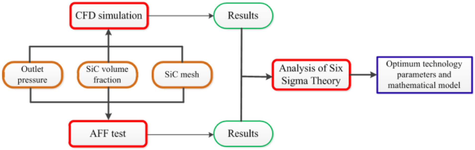
Flow chart showing details of the article.
Numerical simulation
Selection of abrasive flow model
Because the volume fraction of the particles is more than 0.1%, and the dispersion of the particles is wide and the calculation is small, the mixture model is chosen to simulate.
For solid–liquid abrasive flow polishing T-pipe, turbulent flow pattern of fluid has a very important influence on the processing effect. Therefore, it is important to select the appropriate turbulence model to improve the accuracy of numerical simulation. Standard equation turbulence model 23 is a classical model of turbulence. The viscosity coefficient is constant in the equation, and accurate results can be obtained in the whole turbulent flow simulation. But a curved line will be produced, and to a certain extent, the viscosity coefficient will produce distortion due to the existence of curved wall in the T-pipe. Shih and other scholars put forward a model that can be realized, such as formulas (1) and (2) to this problem


where ρ is the density of fluid phase, xi and xj are coordinate components,
Setting of initial condition
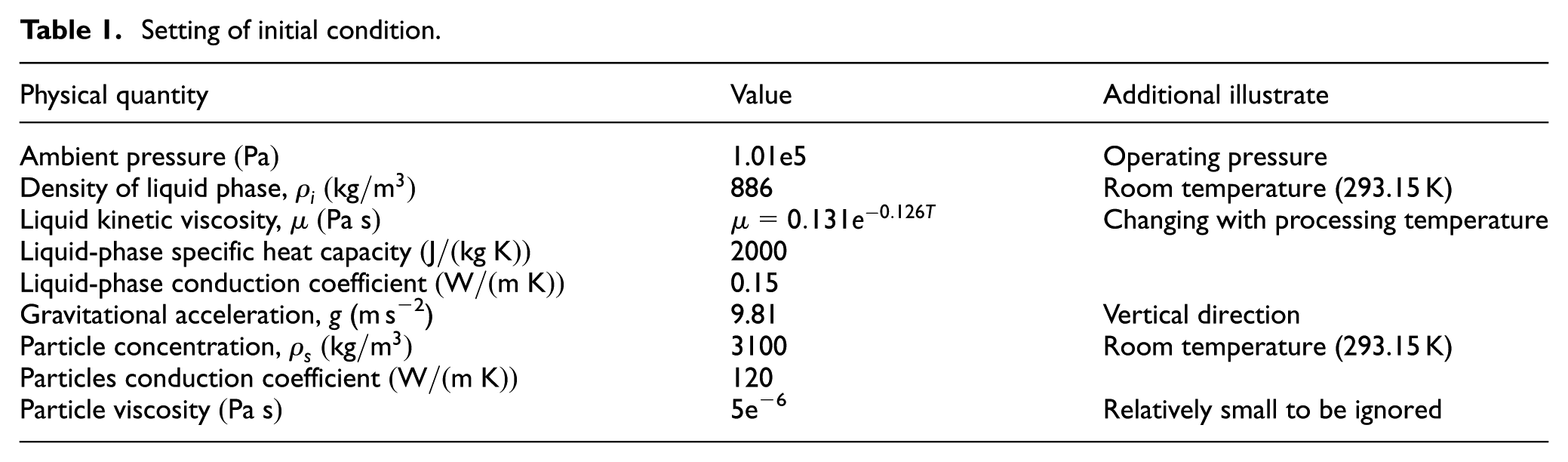
The numerical simulation of near-wall region in T-pipe which is polished by the solid–liquid abrasive flow is carried out. Inlet channel uses import pressure conditions, and inlet pressure is 12 MPa. It is assumed that abrasive flow condition at the inlet is turbulent and then inlet velocity is perpendicular to inlet boundary. The outlet pressure is controlled to keep the pressure difference of the abrasive particles in the T tube; according to the relationship between the flow stress and the material removal rate, 24 the contact stress between the boundary layer and the flow channel wall increases with the increase in the pressure difference, the relative slip becomes more vigorous, and polishing efficiency is improved. Outlet boundary conditions based on actual processing conditions adopt export pressure conditions, which is that outlet pressure is 5, 7, and 9 MPa and silicon carbide volume fraction is 0.25%, 0.3%, and 0.35%. In combination with the actual machining conditions, other initial parameters are set, as shown in Table 1.
Setting of initial condition.
Numerical analysis
According to the T-pipe characteristics, several factors of polishing of internal channel are analyzed and then the distribution of temperature, turbulent viscosity, and turbulent dissipation rate in the polishing process is obtained. For the convenience of observing simulation results, the simulation results on the YOZ surface are analyzed. At the same time, since the change in the turbulent dissipation rate takes place only in the intersection vicinity, partial enlarged drawing of intersection hole is placed the right of simulation cloud image of turbulent dissipation rate, as shown in Figures 3–11.

The distribution of temperature in different SiC volume fractions (outlet pressure is 5 MPa): (a) volume fraction is 0.25%, (b) volume fraction is 0.3%, and (c) volume fraction is 0.35%.

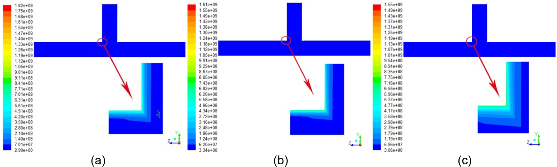
The distribution of turbulent dissipation rates in different SiC volume fractions (outlet pressure is 5 MPa): (a) volume fraction is 0.25%, (b) volume fraction is 0.3%, and (c) volume fraction is 0.35%.

The distribution of turbulence viscosity in different SiC volume fractions (outlet pressure is 5 MPa): (a) volume fraction is 0.25%, (b) volume fraction is 0.3%, and (c) volume fraction is 0.35%.

The distribution of temperature in different SiC volume fractions (outlet pressure is 7 MPa): (a) volume fraction is 0.25%, (b) volume fraction is 0.3%, and (c) volume fraction is 0.35%.

The distribution of turbulent dissipation rates in different SiC volume fractions (outlet pressure is 7 MPa): (a) volume fraction is 0.25%, (b) volume fraction is 0.3%, and (c) volume fraction is 0.35%.

The distribution of turbulence viscosity in different SiC volume fractions (outlet pressure is 7 MPa): (a) volume fraction is 0.25%, (b) volume fraction is 0.3%, and (c) volume fraction is 0.35%.

The distribution of temperature in different SiC volume fractions (outlet pressure is 9 MPa): (a) volume fraction is 0.25%, (b) volume fraction is 0.3%, and (c) volume fraction is 0.35%.
The distribution of turbulent dissipation rates in different SiC volume fractions (outlet pressure is 9 MPa): (a) volume fraction is 0.25%, (b) volume fraction is 0.3%, and (c) volume fraction is 0.35%.

The distribution of turbulence viscosity in different SiC volume fractions (outlet pressure is 9 MPa): (a) volume fraction is 0.25%, (b) volume fraction is 0.3%, and (c) volume fraction is 0.35%.
According to Figures 3–11, analysis results are as follows.
Numerical analysis of the temperature field
From Figures 3, 6, and 9, it is known that temperature changes are mainly concentrated in the intersection vicinity of T-pipe. With the change in SiC volume fraction, the maximum temperature of T-pipe remains basically unchanged. In other words, the volume fraction of silicon carbide has little effect on the distribution of temperature field in the same outlet pressure.
It is shown that, from Figures 3, 6, and 9 followed by the corresponding analysis, in the same volume fraction of SiC, with increasing outlet pressure, maximum temperature near the cross hole decreases gradually and intense particle motion slows down. Therefore, it is preliminary judgment that with difference of inlet and outlet pressure decreases, abrasive flow processing effect has a trend of becoming bad.
Numerical analysis of the turbulent dissipation rate
From Figures 4, 7, and 10, it is illustrated that the change in the turbulence dissipation rate is mainly concentrated in the intersection vicinity of T-pipe. In the same pressure condition, the turbulence dissipation rate and the conversion rate decrease and particle collision intensity slows down with the increase in silicon carbide volume fraction, and polishing effect to the cross hole is poor.
From Figures 4, 7, and 10, it is also shown that in different pressure boundary conditions, the change in the turbulent dissipation rate with the same SiC volume fraction is more obvious, and the effect of pressure on the turbulent dissipation rate is more significant compared with SiC volume fraction. With the increase in the outlet pressure, turbulent dissipation rate decreases sharply, conversion rate decreases obviously, particles movement becomes slow, and processing effect becomes worse.
Numerical simulation of the turbulent viscosity
From Figures 5, 8, and 11, we can know that, due to the movement of SiC abrasive in the turbulent state, the turbulent viscosity increases with the increase in the volume fraction of SiC particles in the same pressure boundary condition. Due to velocity gradient and viscoelasticity of fluid, silicon carbide abrasive particles will inevitably lead to friction of the internal wall. Therefore, it is preliminary judgment that with the increase in SiC volume fraction, the turbulence viscosity increases and processing effect is better.
From Figures 5, 8, and 11, it is also shown that the turbulence viscosity gradually becomes larger with the increase in the pressure of the inlet and outlet in the T-pipe. Therefore, it is preliminary judgment that with the increase in pressure of the import and export, the turbulent viscosity increases sharply, and abrasive flow polishing effect becomes better.
According to the above numerical analysis, we can see that the effect of the SiC volume fraction on the temperature, turbulent viscosity, and turbulent dissipation rate is larger than that of the outlet pressure.
Abrasive flow polishing test and results analysis
In the abrasive flow polishing test, medium composition which is configured according to a certain proportion is made up of solid phase (SiC) and liquid phase (aviation oil).
Design of test scheme
Orthogonal experimental method is used to design the test scheme. And T-pipe outlet pressure, mesh size, and volume fraction of SiC particles are three key parameters to the orthogonal test. To verify the simulation experiment, outlet pressure is set as 5, 7, and 9 MPa; silicon carbide particle mesh is set 80, 100, and 120 mesh; volume fraction of SiC is 0.25%, 0.3%, and 0.35%. Therefore, the test is an orthogonal experiment of three factors and three levels. The design of the concrete test process is shown in Table 2.
Test scheme for abrasive flow machining.
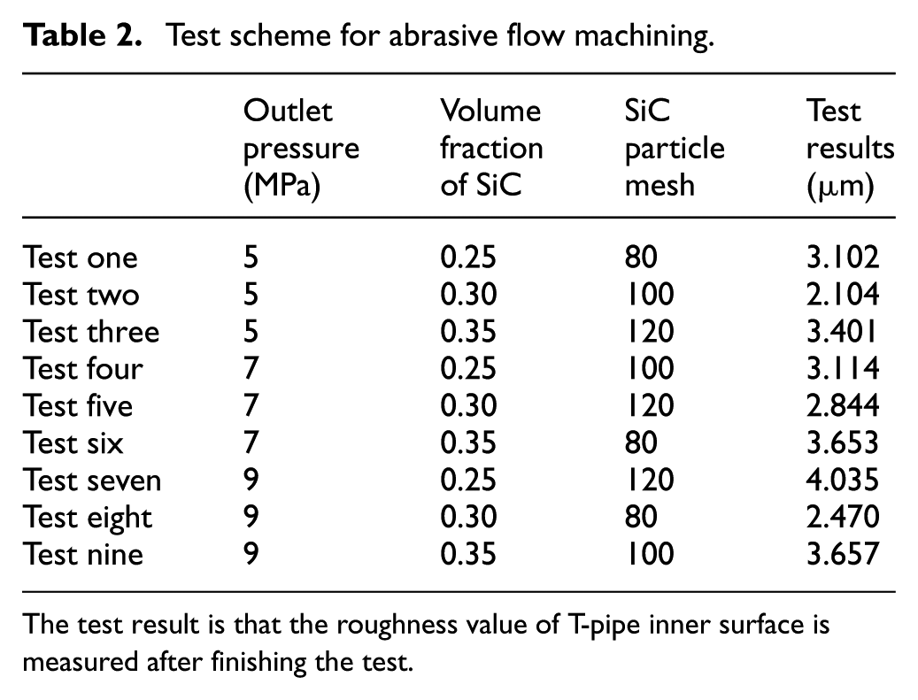
The test result is that the roughness value of T-pipe inner surface is measured after finishing the test.
Test result analysis
According to the orthogonal test scheme, the number of tests is 9 times, and the polishing time is 1 h. After polishing, the surface topography of the T-pipe inner wall before and after polishing is amplified by the electron microscope, and the effect figures are shown in Figure 12. At the same time measuring surface roughness of original and after polishing, detection results are shown in Figure 13. The test results of inner surface roughness are in the fourth column of Table 2.

Surface roughness (a) before and (b) after polishing.

Roughness detection result figures of different T-pipes: (a) the original, (b) Sample 1, (c) Sample 2, (d) Sample 3, (e) Sample 4, (f) Sample 5, (g) Sample 6, (h) Sample 7, (i) Sample 8, and (j) Sample 9.
In Figure 12, pit and microcracks on the surface of the T-pipe inner wall before polishing are shown clearly, and there is a significant improvement after polishing.
Through making a summary of the surface roughness from Figure 13, roughness results (Table 2) can be obtained. The surface roughness of original T-pipe inner wall is 6.603 µm. Therefore, surface roughness of the T-pipe inner wall is significantly reduced after polishing.
Analysis of roughness data
In order to explore the effect of the outlet pressure, mesh size, and volume fraction of SiC on polishing quality, the detection of T-pipe surface roughness was analyzed through Six Sigma Theory. The surface roughness of response mean table is obtained, as shown in Table 3.
Response mean table.

Table 3 shows the average and range (Delta) of each factor. According to the rank of range size, during the polishing T-pipe process, SiC volume fraction is the largest effect factor on polishing quality, followed by the outlet pressure, and finally the SiC mesh. After calculation, the main effect of the T-pipe roughness is obtained, as shown in Figure 14.

Main effect curve of T-pipe surface roughness.
Figure 14 shows that during processing of the T-pipe, the impact order of technological parameters on surface roughness is SiC volume fraction, outlet pressure, and finally SiC mesh.
Then, contour map among surface roughness value, outlet pressure, and SiC volume fraction discussed optimal processing parameters, as shown in Figures 15–17.

The contour map among SiC volume fraction, outlet pressure, and roughness value.

The contour map among SiC mesh, outlet pressure, and roughness value.

The contour map among SiC volume fraction, SiC mesh, and roughness value.
Figure 15 shows that with the increase in outlet pressure, surface roughness becomes larger, and processing effect becomes worse. However, with the increase in silicon carbide volume fraction, roughness values decrease first and then increase. Especially when the volume fraction of silicon carbide is 0.3, the processing effect is the best, and then the outlet pressure is 5 MPa.
Figure 16 shows that with the increase in outlet pressure, surface roughness increases first and then decreases. With the increase in SiC mesh, surface roughness decreases first and then increases. Especially when SiC mesh is 100 and outlet pressure is 5 MPa, processing effect is the best.
Figure 17 shows that when volume fraction of silicon carbide is 0.3 and SiC mesh is 100, processing effect is the best, which verifies the conclusions from Figures 15 and 16.
According to the above discussions, the optimum process parameters for abrasive flow polishing T-pipe are obtained: outlet pressure is 5 MPa, SiC volume fraction is 0.3, and SiC mesh is 100.
Establishing surface roughness prediction model
Roughness and three factors (outlet pressure, volume fraction of SiC, and SiC mesh) are fitted by three-element polynomial fitting. In addition to that, quadratic regression polynomial analysis is also performed among roughness, respectively, with outlet pressure, SiC volume fraction, and SiC mesh (Table 4). According to the above fitting, it is found that when roughness and SiC volume fraction are fitted by quadratic regression polynomial analysis, the p value is less than 0.05, and the value of R2 is more reasonable. For other fitting, the value of p is more than 0.05 and R2 value is not reasonable, which results in a larger error.
Quadratic regression polynomial analysis: variance analysis between roughness and SiC volume fraction.

DOF: degree of freedom; SS: Stdev square; MS: mean square.
Correlation coefficient and S value of the model are obtained from Table 4: S = 0.460454, R2 = 74.2%, and R2 (adjusted) = 62.4%.
For linear and quadratic regression fitting model in Table 5, it is can be seen that the p value of quadratic regression model is less than 0.05 and the value of R2 is more reasonable with small error.
Quadratic regression polynomial analysis: variance analysis between roughness and SiC volume fraction after optimized.

DOF: degree of freedom; SS: Stdev square; MS: mean square.
In addition, the model needs to verify reliability by residual error, as shown in Figure 18.

Roughness of residual figure.
It can be seen from Figure 18 that the residual is not maintained and the distribution of each point of observation sequence is a funnel shape, which suggests that the residual error is more reasonable after a transformation. So taking a new response variable, the effect will be better. The model is optimized by the Box-Cox transform, and the new mathematical model of the variance analysis table is obtained, as shown in Table 5.
Correlation coefficient and S value of the model are obtained from Table 5: S = 0.0613430, R2 = 82.5%, and R2 (adjusted) = 73.1%. Comparing Tables 4 and 5, it can be seen that, after the Box-Cox transform, the value of R2 changes from 74.2% to 82.5%, and R2 (adjusted) changes from 62.4% to 73.1%. The values of R2 and R2 (adjusted) are significantly larger, which shows that the optimized model has been improved. The p value decreases from 0.046 to 0.031, which illustrates that the fitting effect becomes better.
Then, model will be verified reliably by residual diagnosis, as shown in Figure 19.

Roughness of residual figure after optimizing.
Figure 19 shows that the funnel shape in Figure 18 disappeared, which illustrates that after Box-Cox transformation the model has a very good expression for test results, as well as the establishment of a mathematical model is reliable and reasonable.
Finally, fitting model of surface roughness and SiC volume fraction can be obtained by Six Sigma Theory, such as equation (3)

where
Conclusion
T-pipe is the research object, on abrasive flow polishing process numerical simulation of outlet pressure, the mesh SiC volume fraction, and silicon carbide three parameters of wear particle flow research the effect of the polishing quality. Through the numerical analysis, it is found that the volume fraction of silicon carbide is the biggest, and the second is the outlet pressure.
Based on the numerical simulation, the experimental scheme is designed by the orthogonal design method. The effectiveness of abrasive flow machining can be found through the detection of the surface roughness of the T-pipe.
The surface roughness was obtained using Six Sigma Theory to analyze the surface roughness of the three pipes. From the size of the range rank we can know that, during the polishing three-way pipe process, polishing quality influence is the largest silicon carbide volume fraction, followed by the outlet pressure, and finally the mesh of silicon carbide. Finally, we get the corresponding mean response table, the main effect diagram, the surface map, and the contour map. And abrasive flow research throws the three-way pipe of optimum process parameters: outlet pressure of 5 MPa, the volume fraction of SiC is 0.3, and the mesh of silicon carbide is 100.
Six Sigma Theory is used to fit the regression equation and then the test data are optimized. Finally, the mathematical model is established under the condition of this experiment.
Footnotes
Academic Editor: Jun Ren
Declaration of conflicting interests
The author(s) declared no potential conflicts of interest with respect to the research, authorship, and/or publication of this article.
Funding
The author(s) disclosed receipt of the following financial support for the research, authorship, and/or publication of this article: This work was supported by the National Natural Science Foundation of China (No. NSFC 51206011), Jilin Province Science and Technology Development Program of Jilin Province (Nos 20160101270JC and 20170204064GX), and project of Education Department of Jilin Province (No. 2016386).