Concise method to the dynamic modeling of climbing robot

Abstract

With the aim of dynamic modeling of the climbing robot with dual-cavity structure and wheeled locomotion mechanism, a succinct and explicit equation of motion based on the Udwadia–Kalaba equation is established. The trajectory constraint of the climbing robot, which is regarded as the external constraint of the system, is integrated into the dynamic equation dexterously. A modified numerical method is considered to reduce the errors because the numerical results obtained by integrating the constrained dynamic equation yield the errors. The trajectories are almost coincident by comparing the modified numerical value and the theoretical value. The driving torques required to guarantee the climbing robot to move along the given trajectory are obtained explicitly, which overcomes the disadvantage of obtaining dynamical equation from traditional Lagrange equation by Lagrange multiplier. The simulations are performed to demonstrate that the dynamical equation established by this method with brevity and accuracy is in accordance with reality status.

Introduction

Climbing robots have been a very attractive research topic since there are various potential applications to increase operational efficiency and protect human health and safety in environments such as the exteriors of buildings, bridges or dams storage tanks, nuclear facilities, and reconnaissance within building. In general, climbing robots can be categorized based on the surface adhesion (e.g. magnetic type, ¹ gripping type, ² rail guided type, ³ biomimetic type, ⁴ and suction type ⁵ ) and the locomotion mechanism (e.g. legged type, ⁶ tracked type, ⁷ translation type, ³ cable-driven type, ⁸ and wheeled type ⁹ ), which are the two major issues in the design of climbing robots. Suction adhesion, which is the most commonly used adhesion method, can be widely adopted for less rough surfaces because it enables strong attachment to the surfaces regardless of materials such as glass, ceramics tiles, and cement. Using wheeled type as the locomotive mechanism, the robots have high moving speed, simple structure, and feasible control system.

For climbing robot, the accurate kinematics and dynamical models are the basis for completing all kinds of tasks. F Xu et al. ¹⁰ derived the kinematics and dynamical models for the obstacle-climbing capabilities of the driving and driven wheels of the robot; WR Provancher et al. ¹¹ developed the dynamical model of the city-climber robot that has the capability to move on floors, climb walls, walk on ceilings, and transit between them when it travels on different surfaces. WH Ko et al. ¹² simplified and redeveloped the reduced-order two-arm dynamic model on climbing robot (i.e. not computer-aided design (CAD) model or kinematic model) based on Lagrangian mechanics to explore the relation between the individual model parameters and the resultant dynamic behavior of the model. S Nam et al. ¹³ derived the dynamics model of a compliant multibody climbing robot with magnetic adhesion using the Lagrangian formulation. However, the processes of above-mentioned dynamic modeling are complex and complicated.

Obtaining equations of motion for constrained mechanical systems is one of the central issues in multibody dynamics. ¹⁴ Constrained motion was initially described by Lagrange in 1787 using Lagrange multiplier method, which relies on problem-specific approaches to determine the multipliers that are often very difficult to find. Gauss’ principle was proposed by Gauss in 1829 which gives a clear description of the general nature of constrained motion through minimization of a function of the accelerations of the particles of a system. Gibbs ¹⁵ and Appell ¹⁶ had independently developed equations of constrained motion when the constraints satisfy d’Alembert’s principle in 1879 and 1899, respectively. However, Gibbs–Appell equations require specific quasi-coordinates. Dirac ¹⁷ developed how to determine the Lagrange multipliers using Poisson brackets for singular Hamiltonian systems in 1964, in which the constraints do not exactly depend on time. There are some marvelous discoveries, called the Udwadia–Kalaba equation, proposed by Firdaus E. Udwadia and Robert E. Kalaba from the University of Southern California in 1992. The significant advantages are threefold. (1) The governing motion equations of multibody system subject to holonomic constraints are proposed based on d’Alembert’s principle and Gauss’ principle.^18,19 (2) Given that the system with nonideal constraints may not satisfy d’Alembert’s principle, explicit set of equations under the case of nonholonomic constraints are added to perfect the previous motion equations of multibody system.^20,21 (3) General and explicit equations of motion to handle systems whether or not their mass matrices are singular are developed in the case of singular mass matrices arise. The new theory opens up a new way of modeling complex multibody systems. An additional perspective has been proposed by Udwadia and Kalaba which is useful to help us understand nature’s law from new points of view.

The explicit equations of constraint force without Lagrange multiplier can be obtained according to Udwadia–Kalaba theory, which is a simple, aesthetic, and thought-provoking description of the world at a very fundamental level, to realize a great breakthrough in the field of analytical mechanics.^18,22–24 Udwadia and colleagues^24–27 also successfully addressed the dynamics and control of nonlinear uncertain systems using the fundamental equation to provide considerable reference value for the basic research and the further application of this method. Many researchers have studied and established dynamical model in some application fields by employing the Udwadia–Kalaba approach, such as satellite systems, ²⁸ industry mechanical arm, ²⁹ parallel manipulator, ³⁰ flexible multibody systems, ³¹ machine fish, ¹⁴ heavenly bodies’ movements (especially on Kepler’s law and the inverse square law of gravitation), ³² and falling cat’s movements. ³³

In view of its strong attachment to the surfaces, high moving speed and simple control system, climbing robot based on dual-cavity structure and wheeled locomotion mechanism is studied in this article. Like many other robots, climbing robots are often required to move along some specified trajectories (i.e. trajectory constraint). However, only a few scholars focus on the explicit dynamical equations for climbing robot subject to constrains.

In this article, a succinct and exact dynamic modeling of constrained climbing robot is presented by applying the Udwadia–Kalaba approach. However, the numerical results obtained by integrating the constrained dynamic equation yield the errors. Therefore, a modified numerical method is considered to reduce the errors. Numerical simulations are performed to demonstrate the efficacy and accuracy of this method. Finally, conclusions of this work and the future tasks are given.

Udwadia–Kalaba equation

This section shows how to obtain the explicit equations of motion for a constrained dynamical system using a simple straightforward three-step procedure:^18,24

1. In terms of the generalized coordinates, equations of motion of the unconstrained dynamical system written using Newtonian or Lagrangian mechanics are considered.

2. Trajectory constraint required to model of the given constrained system is described.

3. Additional generalized forces of constraint imposed on the system are expressed.

Step 1: unconstrained dynamics

Consider an unconstrained dynamical system, the configuration of which is uniquely specified by the n generalized coordinates $\mathbf{q}:=[q_1{q}_2\cdots q_n{]}^T$ , in which the superscript T represents the transpose of a vector or a matrix. Using Newtonian or Lagrange equation, the equation of unconstrained motion of the system can be expressed in the following form ²⁴

$$M\left(q,t\right)\stackrel{\mathrm{··}}{q}=Q(q,\stackrel{.}{q},t)$$

(1)

with the initial conditions

$$\mathbf{q}\left(0\right)={\mathbf{q}}_0,\stackrel{·}{\mathbf{q}}\left(0\right)={\stackrel{·}{\mathbf{q}}}_0$$

(2)

in which $\mathbf{M}(\mathbf{q},t)\in {\mathbb{R}}^{n\times n}$ is a mass matrix, which is a function of $\mathbf{q}$ and t; $\mathbf{Q}(\mathbf{q},\stackrel{·}{\mathbf{q}},t)\in {\mathbb{R}}^n$ collects the normal and Coriolis inertial terms and the applied forces and is a known function of $\mathbf{q}$ , $\stackrel{·}{\mathbf{q}}$ , and t; $\mathbf{q}\in {\mathbb{R}}^n$ is the generalized coordinate n-vector; $\stackrel{·}{\mathbf{q}}\in {\mathbb{R}}^n$ is the velocity; $\stackrel{··}{\mathbf{q}}\in {\mathbb{R}}^n$ is the acceleration. From equation (1), the generalized acceleration of the unconstrained dynamical system is denoted by $\mathbf{a}(\mathbf{q},\stackrel{·}{\mathbf{q}},t)$ , which is of the form

$$\stackrel{··}{\mathbf{q}}={\mathbf{M}}^{-1}(\mathbf{q},t)\mathbf{Q}(\mathbf{q},\stackrel{·}{\mathbf{q}},t):=\mathbf{a}(\mathbf{q},\stackrel{·}{\mathbf{q}},t)$$

(3)

Step 2: constraint description

The system is subjected to the p sufficiently smooth control requirements as constraints provided by

$${\phi }_i(\mathbf{q},\stackrel{·}{\mathbf{q}},t)=0,i=1,2,\dots ,p$$

(4)

These p constraints include all the usual varieties of holonomic and/or nonholonomic constraints and then some. ²⁴ Equation (4) can be simplified as

$$\mathbf{\Phi }={\left[\begin{array}{cccc}{\phi }_1\hfill & {\phi }_2\hfill & \cdots \hfill & {\phi }_p\hfill \end{array}\right]}^T$$

(5)

Differentiating the usual constraint equation (5) in Lagrangian mechanics which are usually in Pfaffian form with respect to time t once (for nonholonomic constraints) or twice (for holonomic constraints) yields the following set of consistent constraint equations ²⁴

$$\mathbf{A}(\mathbf{q},\stackrel{·}{\mathbf{q}},t)\stackrel{··}{\mathbf{q}}={\mathbf{b}}_v(\mathbf{q},\stackrel{·}{\mathbf{q}},t)$$

(6)

in which $\mathbf{A}(\mathbf{q},\stackrel{·}{\mathbf{q}},t)\in {\mathbb{R}}^{p\times n}$ is referred to as constraint matrix and ${\mathbf{b}}_v(\mathbf{q},\stackrel{·}{\mathbf{q}},t)$ is a p-vector.

The second-order constraint is linear in $\stackrel{··}{\mathbf{q}}$ so that it is believed to be the most appropriate form for further dynamic analysis and ensure the completeness of the information.

Step 3: constraint force description

Additional constrained forces arise due to the constraints applied to the unconstrained system. Accordingly, the actual explicit equation of motion of the constrained system could be assumed to take the form

$$\mathbf{M}(\mathbf{q},t)\stackrel{··}{\mathbf{q}}=\mathbf{Q}(\mathbf{q},\stackrel{·}{\mathbf{q}},t)+{\mathbf{Q}}^{\mathbf{c}}(\mathbf{q},\stackrel{·}{\mathbf{q}},t)$$

(7)

in which ${\mathbf{Q}}^{\mathbf{c}}(\mathbf{q},\stackrel{·}{\mathbf{q}},t)\in {\mathbb{R}}^n$ is the additional constraint force imposed on the system to ensure the control requirements in equation (6) are satisfied. There are already many ways to determine ${\mathbf{Q}}^{\mathbf{c}}(\mathbf{q},\stackrel{·}{\mathbf{q}},t)$ , and recently, a simple and insightful approach was proposed by Udwadia and colleagues^21–27 based on Gauss’ principle of least constraint, which gives the constraint force ${\mathbf{Q}}^{\mathbf{c}}(\mathbf{q},\stackrel{·}{\mathbf{q}},t)$ explicitly as^21,22,34,35

$$\begin{array}{l}{Q}^c\left(t\right):=Q^c\left(q,\stackrel{.}{q},t\right)\\ =M^{\frac{1}{2}}(q)B^{+}\left(q,t\right)\left(b_v\left(q,\stackrel{.}{q},t\right)-A\left(q,\stackrel{.}{q},t\right)M^{-1}\left(q\right)Q\left(q,\stackrel{.}{q},t\right)\right)\end{array}$$

(8)

in which $\mathbf{B}(\mathbf{q},t)=\mathbf{A}(\mathbf{q},\stackrel{·}{\mathbf{q}},t){\mathbf{M}}^{-\frac{1}{2}}(\mathbf{q})$ , and the superscript “+” represents the generalized Moore–Penrose inverse. The exact control force ${\mathbf{Q}}^{\mathbf{c}}(\mathbf{q},\stackrel{·}{\mathbf{q}},t)$ , which minimizes the quantity $[{\mathbf{Q}}^{\mathbf{c}}(\mathbf{q},\stackrel{·}{\mathbf{q}},t){]}^T{\mathbf{M}}^{-1}[{\mathbf{Q}}^{\mathbf{c}}(\mathbf{q},\stackrel{·}{\mathbf{q}},t)]$ at each instant of time t, enables all the constraints to be exactly satisfied at every instant of time t and can be derived explicitly by equation (8).

Accordingly, the explicit dynamical equation of the constrained system is shown in the following general form

$$\begin{array}{l}M\left(q\right)\stackrel{\mathrm{··}}{q}=Q\left(q,\stackrel{.}{q},t\right)\\ +M^{\frac{1}{2}}\left(q\right)B^{+}\left(q,t\right)\left[b_v\left(q,\stackrel{.}{q},t\right)-A\left(q,\stackrel{.}{q},t\right)M^{-1}\left(q\right)Q\left(q,\stackrel{.}{q},t\right)\right]\end{array}$$

(9)

In this article, equation (9) is referred to as the Udwadia–Kalaba equation. Premultiplying both sides of equation (9) with ${\mathbf{M}}^{-1}$ , the acceleration of the constrained system can be obtained by

$$\begin{array}{l}\stackrel{\mathrm{··}}{q}:=a+M^{-1}{Q}^c=M^{-1}Q+M^{-\frac{1}{2}}{\left(A{M}^{-\frac{1}{2}}\right)}^{+}\\ \left(b_v-A{M}^{-1}Q\right)\end{array}$$

(10)

Dynamic modeling of climbing robot

This section develops the dynamic model of the climbing robot with dual-cavity structure and wheeled locomotion mechanism. Dual cavities are adsorbed on the wall with negative pressure absorption. As the driving wheels, the two rear wheels are driven by two DC servo motors, respectively, while the power is transmitted to the two front wheels by synchronous belt. Four-wheel move steering mechanisms are employed to enhance the driving forces on the wall. Several important assumptions are made to simplify the modeling:

1. The climbing robot is considered to be a single rigid body.

2. The center of mass is in the geometric center of the climbing robot.

3. There is no-slip motion on the wheels.

4. The moment of inertia of the wheels and the rolling friction between the wheels and the wall are ignored.

5. The friction between the seal ring and the wall distributes on the center of the robot with uniformity and symmetry.

6. The climbing robot is symmetrical, so the force analysis model is simplified as a two-dimensional (2D) model.

Consider an inertial frame of reference XOY in which a climbing robot of mass m (with center of mass is at o) moves on the 2D surface (see Figure 1). The generalized coordinates $\mathbf{q}=[x,y,\theta {]}^T$ are denoted as the configuration of the mass center of the climbing robot. In which v is the velocity of the climbing robot; $\theta$ is the orientation angle of the climbing robot; $F_R$ and $F_L$ are the forces produced by the right and left motors, respectively; f is the friction between the seal ring and the wall; $G_1$ is the gravity component in the v-direction; J is the moment of inertia around the mass center of the climbing robot; and d is the distance between the right or left wheel and the mass center of the climbing robot.

Figure 1.

Climbing robot subject to trajectory constraint.

Explicit dynamic modeling

• 1. According to Newton’s second law of motion, the following relation can be obtained

$$m\stackrel{·}{v}=F_R+F_L-G_1-f$$

(11)

The different forces in equation (11) can be given as $F_R={\tau }_R/r$ , $F_L={\tau }_L/r$ , $G_1=\mathrm{mg}\sin \theta$ , $f=(1-k){\mu }_M{F}_S$ , and $F_S=\mathrm{PS}$ , in which ${\tau }_R$ and ${\tau }_L$ are the driving torques of the right and left motors, respectively; r is the radius of the wheels; k is the ratio of the pressure on the wheels to the pressure on the whole robot; ${\mu }_M$ is the coefficient of rolling resistance between the tracked wheels and wall; P is the pressure difference between the atmospheric pressure and the pressure inside the seal ring; and S is the effective adsorption area of the seal ring.

The velocity of the climbing robot in the generalized coordinates $q=[x,y,\theta {]}^T$ can be expressed as

$$v=\stackrel{·}{x}\cos \theta +\stackrel{·}{y}\sin \theta$$

(12)

and the acceleration of the climbing robot can be represented by

$$\stackrel{·}{v}=\stackrel{··}{x}\cos \theta +\stackrel{··}{y}\sin \theta -\stackrel{·}{x}\sin \theta \stackrel{·}{\theta }+\stackrel{·}{y}\cos \theta \stackrel{·}{\theta }$$

(13)

in which $\stackrel{·}{x}$ and $\stackrel{·}{y}$ are the velocities of the mass center of the climbing robot in the X- and Y-directions, respectively; and $\stackrel{··}{x}$ and $\stackrel{··}{y}$ are the accelerations of the mass center of the climbing robot in the X- and Y-directions, respectively.

Substituting equation (13) into equation (11), the following equation is derived

$$\begin{array}{l}mr\cos \theta \stackrel{··}{x}+mr\sin \theta \stackrel{··}{y}=mr\sin \theta \stackrel{.}{\theta }\stackrel{.}{x}-mr\cos \theta \stackrel{.}{\theta }\stackrel{.}{y}\\ +{\tau }_R+{\tau }_L-fr-mgr\sin \theta \end{array}$$

(14)

• 2. The momentum balance can be written as

$$J\stackrel{··}{\theta }=F_{R}d-F_{L}d$$

(15)

or, equivalently

$$\frac{\mathrm{Jr}}{d}\stackrel{··}{\theta }={\tau }_R-{\tau }_L$$

(16)

• 3. The structural constraint of the climbing robot is expressed as

$$\stackrel{·}{x}\sin \theta -\stackrel{·}{y}\cos \theta =0$$

(17)

Differentiating equation (17) with respect to t yields

$$\sin \theta \stackrel{··}{x}-\cos \theta \stackrel{··}{y}=-\cos \theta \stackrel{·}{\theta }\stackrel{·}{x}-\sin \theta \stackrel{·}{\theta }\stackrel{·}{y}$$

(18)

Accordingly, equations (14), (16), and (18) can be expressed in matrix equation

$$\begin{array}{c}\left[\begin{array}{ccc}\mathrm{mr}\cos \theta \hfill & \mathrm{mr}\sin \theta \hfill & 0\hfill \\ \multicolumn{1}{c}{0}& 0\hfill & \frac{\mathrm{Jr}}{d}\hfill \\ \multicolumn{1}{c}{\sin \theta }& -\cos \theta \hfill & 0\hfill \end{array}\right]\left[\begin{array}{c}\stackrel{··}{x}\hfill \\ \multicolumn{1}{c}{\stackrel{··}{y}}\\ \multicolumn{1}{c}{\stackrel{··}{\theta }}\end{array}\right]\hfill \\ =\left[\begin{array}{c}\mathrm{mr}\sin \theta \stackrel{·}{\theta }\stackrel{·}{x}-\mathrm{mr}\cos \theta \stackrel{·}{\theta }\stackrel{·}{y}-\mathrm{fr}-\mathrm{mgr}\sin \theta \hfill \\ \multicolumn{1}{c}{0}\\ \multicolumn{1}{c}{-\cos \theta \stackrel{·}{\theta }\stackrel{·}{x}-\sin \theta \stackrel{·}{\theta }\stackrel{·}{y}}\end{array}\right]\hfill \\ +\left[\begin{array}{cc}1\hfill & 1\hfill \\ \multicolumn{1}{c}{1}& -1\hfill \\ \multicolumn{1}{c}{0}& 0\hfill \end{array}\right]\left[\begin{array}{c}{\tau }_R\hfill \\ \multicolumn{1}{c}{{\tau }_L}\end{array}\right]\hfill \end{array}$$

(19)

Equation (19) can be simplified as

$$\mathbf{M}\left(\mathbf{q}\right)\stackrel{··}{\mathbf{q}}=\mathbf{Q}(\mathbf{q},\stackrel{·}{\mathbf{q}},t)+{\mathbf{Q}}^{\mathbf{c}}(\mathbf{q},\stackrel{·}{\mathbf{q}},t)$$

(20)

in which

$$\begin{array}{c}\mathbf{q}=\left[\begin{array}{c}x\hfill \\ \multicolumn{1}{c}{y}\\ \multicolumn{1}{c}{\theta }\end{array}\right],\stackrel{·}{\mathbf{q}}=\left[\begin{array}{c}\stackrel{·}{x}\hfill \\ \multicolumn{1}{c}{\stackrel{·}{y}}\\ \multicolumn{1}{c}{\stackrel{·}{\theta }}\end{array}\right],\stackrel{··}{\mathbf{q}}=\left[\begin{array}{c}\stackrel{··}{x}\hfill \\ \multicolumn{1}{c}{\stackrel{··}{y}}\\ \multicolumn{1}{c}{\stackrel{··}{\theta }}\end{array}\right]\hfill \\ \mathbf{M}\left(\mathbf{q}\right)=\left[\begin{array}{ccc}\mathrm{mr}\cos \theta \hfill & \mathrm{mr}\sin \theta \hfill & 0\hfill \\ \multicolumn{1}{c}{0}& 0\hfill & \frac{\mathrm{Jr}}{d}\hfill \\ \multicolumn{1}{c}{\sin \theta }& -\cos \theta \hfill & 0\hfill \end{array}\right]\hfill \\ \mathbf{Q}=\left[\begin{array}{c}\mathrm{mr}\sin \theta \stackrel{·}{\theta }\stackrel{·}{x}-\mathrm{mr}\cos \theta \stackrel{·}{\theta }\stackrel{·}{y}-\mathrm{fr}-\mathrm{mgr}\sin \theta \hfill \\ \multicolumn{1}{c}{0}\\ \multicolumn{1}{c}{-\cos \theta \stackrel{·}{\theta }\stackrel{·}{x}-\sin \theta \stackrel{·}{\theta }\stackrel{·}{y}}\end{array}\right]\hfill \\ {\mathbf{Q}}^{\mathbf{c}}=\left[\begin{array}{cc}1\hfill & 1\hfill \\ \multicolumn{1}{c}{1}& -1\hfill \\ \multicolumn{1}{c}{0}& 0\hfill \end{array}\right]\left[\begin{array}{c}{\tau }_R\hfill \\ \multicolumn{1}{c}{{\tau }_L}\end{array}\right]\hfill \end{array}$$

in which ${\mathbf{Q}}^{\mathbf{c}}$ is the constraint force to satisfy the trajectory constraint as described below.

Trajectory constraint description

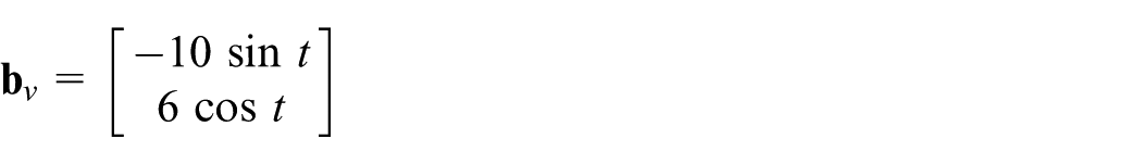
The climbing robot moves on the wall along the following trajectory to perform specific tasks. The constrained trajectory is expressed as

$$\{\begin{array}{c}x=10\sin t\hfill \\ \multicolumn{1}{c}{y=-6\cos t}\end{array}$$

(21)

Differentiating equation (21) with respect to time t twice yields the second-order constrains

$$\{\begin{array}{c}\stackrel{··}{x}=-10\sin t\hfill \\ \multicolumn{1}{c}{\stackrel{··}{y}=6\cos t}\end{array}$$

(22)

Equation (22) can be simplified as

$$\mathbf{A}\stackrel{··}{\mathbf{q}}={\mathbf{b}}_v$$

(23)

in which

$$\mathbf{A}=\left[\begin{array}{ccc}1\hfill & 0\hfill & 0\hfill \\ \multicolumn{1}{c}{0}& 1\hfill & 0\hfill \end{array}\right]$$

$$\stackrel{··}{\mathbf{q}}=\left[\begin{array}{c}\stackrel{··}{x}\hfill \\ \multicolumn{1}{c}{\stackrel{··}{y}}\\ \multicolumn{1}{c}{\stackrel{··}{\theta }}\end{array}\right]$$

and

$${\mathbf{b}}_v=\left[\begin{array}{c}-10\sin t\hfill \\ \multicolumn{1}{c}{6\cos t}\end{array}\right]$$

Constraint force description

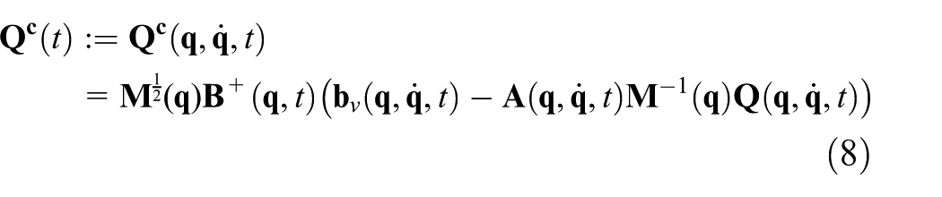
Using equation (8), the constraint torque ${\mathbf{Q}}^{\mathbf{c}}$ , which is equivalent to the constraint force, can be derived as

$$\begin{array}{l}{Q}^c=M^{\frac{1}{2}}{\left(A{M}^{-\frac{1}{2}}\right)}^{+}\left(b_v-A{M}^{-1}Q\right)\\ =\left[\begin{array}{cc}1& 1\\ 1& -1\\ 0& 0\end{array}\right]\left[\begin{array}{c}{\tau }_R\\ {\tau }_L\end{array}\right]=\mathbf{\delta }\mathbf{\tau }\end{array}$$

(24)

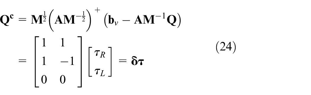
Therefore, the driving torques of the right and left motors $\mathbf{\tau }$ based on Udwadia–Kalaba equation can be obtained as

$$\mathbf{\tau }={\mathbf{\delta }}^{+}{\mathbf{M}}^{\frac{1}{2}}{\left(\mathbf{A}{\mathbf{M}}^{-\frac{1}{2}}\right)}^{+}({\mathbf{b}}_v-\mathbf{A}{\mathbf{M}}^{-1}\mathbf{Q})$$

(25)

Result and simulation analysis

Assuming the initial configurations are $x(0)=0$ , $y(0)=-6$ , $\theta (0)=0$ ; $\stackrel{·}{x}(0)=10$ , $\stackrel{·}{y}(0)=0$ , $\stackrel{·}{\theta }(0)=6/10$ . The parameters for simulation are $m=5\mathrm{kg}$ , $J=0.33\mathrm{kg}{\mathrm{m}}^2$ , $r=0.027\mathrm{m}$ , $d=0.3\mathrm{m}$ , ${\mu }_M=0.8$ , $k=0.53$ , $P=2.5\mathrm{kPa}$ , and $S=0.06{\mathrm{m}}^2$ . The solution of the equations can be obtained through ode45 algorithm in MATLAB 2010b. The error tolerance is set to 10⁻¹² and the simulation time is 20 s. The explicit analytic results given in Figures 2–6 are verified by numerical simulations:

1. Figures 2 and 3 represent x-coordinate curve and y-coordinate curve as a function of time t when a certain level driving torque obtained from equation (25) is generated by the two rear wheels to realize the desired trajectory, in which the solid curves and the dashed curves represent the numerical value and the theoretical value, respectively. x-num and y-num are numerical values of x-coordinate and y-coordinate, respectively.

2. There are obvious errors as a function of time t for the trajectory constraint described by equation (21) between numerical value and theoretical value, even though the solid curve approximates the dashed curve in Figures 2 and 3, as shown in Figures 4 and 5. x-error and y-errors are errors between numerical value and theoretical value of x-coordinate and y-coordinate, respectively. Compared with x = 10 m and y = 6 m, however, the obvious displacement errors, which is about 1.8 × 10⁻³ m in the x-direction and 0.6 m in the y-direction, still exist and increase with time.

3. The numerical trajectories are slightly off the theoretical trajectory with time, as illustrated in Figure 6, in which the solid curve and the dashed curve represent the numerical trajectory and the theoretical trajectory, respectively. Therefore, it is necessary to consider the numerical method for reducing the errors.

Figure 2.

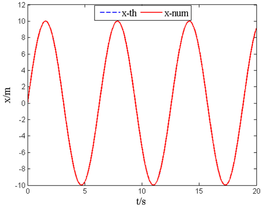
Comparison of x-coordinate curves between numerical value and theoretical value.

Figure 3.

Comparison of y-coordinate curves between numerical value and theoretical value.

Figure 4.

Error curve of x-coordinate between numerical value and theoretical value.

Figure 5.

Error curve in y-coordinate between numerical value and theoretical value.

Figure 6.

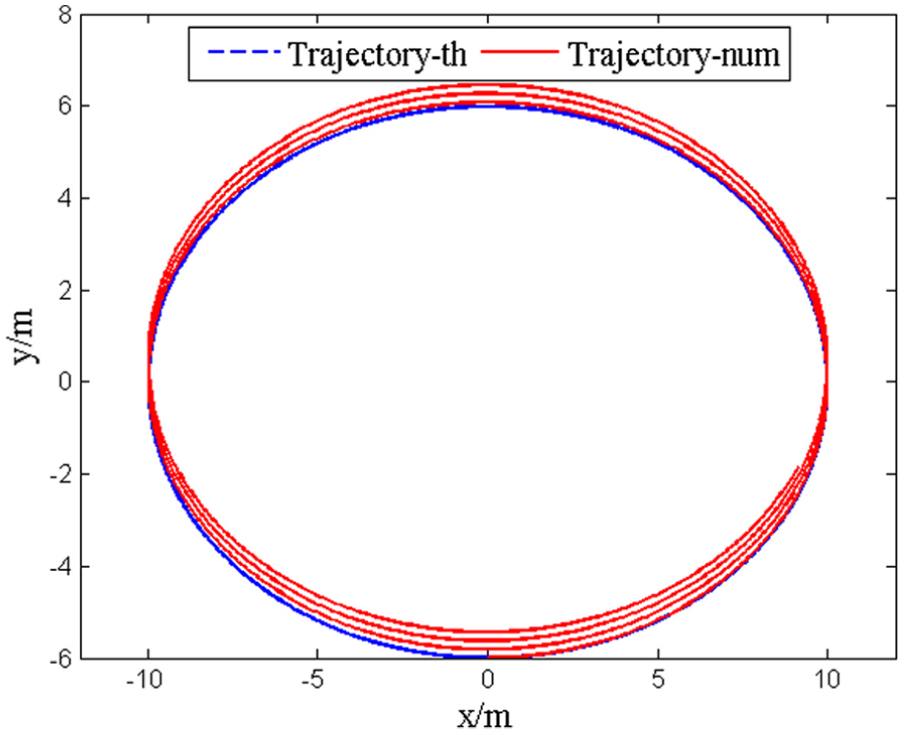
Comparison of trajectories between numerical value and theoretical value.

Errors reducing

Any numerical integration scheme on the second-order differential equation needs a set of two first-order differential equations. ³⁶ One can define the constrained acceleration, $\stackrel{··}{\mathbf{q}}=\stackrel{·}{\mathbf{v}}$ , and rewrite the equation of motion based on the second-order differential equation of equation (10) in the following first-order form

$$\begin{array}{c}\stackrel{·}{\mathbf{q}}=\mathbf{v}\hfill \\ \stackrel{·}{\mathbf{v}}=\mathbf{a}+{\mathbf{M}}^{-\frac{1}{2}}{\mathbf{B}}^{+}({\mathbf{b}}_v-\mathbf{Aa})\hfill \end{array}$$

(26)

It is known that the responses of the constrained dynamic system must satisfy the constraint equations at all times during numerical integration of the dynamic equation. However, it is found that the numerical results tend to deviate from the constrained path as shown in Figure 6. The basic idea for this numerical algorithm for reducing errors is to include the constraint effect into equation (26). It is considered that the errors appeared because the derived dynamic equation (see equation (6)) considers only the acceleration-based constraint and neglects the velocity-based constraint of given trajectory constraints that differentiate the constraint equations once with respect to time. It can be expressed as

$$\mathbf{A}\stackrel{·}{\mathbf{q}}={\mathbf{b}}_q$$

(27)

With the aim of incorporating this error source, one can add a new term considered as a kinematic correction term to equation (26) to compensate for numerical errors along the integration ³⁷

$$\stackrel{·}{\mathbf{q}}=\mathbf{v}+{\mathbf{M}}^{-1}{\mathbf{A}}^T\mathbf{\mu }$$

(28)

Substituting equation (28) into equation (27), one obtains

$$\mathbf{\mu }={\left(\mathbf{A}{\mathbf{M}}^{-1}{\mathbf{A}}^T\right)}^{-1}({\mathbf{b}}_q-\mathbf{Av})$$

(29)

Then, the dynamic equation can be modified as

$$\begin{array}{c}\stackrel{·}{\mathbf{q}}=\mathbf{v}+{\mathbf{M}}^{-1/2}{\mathbf{B}}^{+}({\mathbf{b}}_q-\mathbf{Av})\hfill \\ \stackrel{·}{\mathbf{v}}=\mathbf{a}+{\mathbf{M}}^{-1/2}{\mathbf{B}}^{+}({\mathbf{b}}_v-\mathbf{Aa})\hfill \end{array}$$

(30)

in which $\stackrel{·}{\mathbf{q}}$ is the constrained velocity, $\mathbf{v}$ is the constrained acceleration, and $\mathbf{a}={\mathbf{M}}^{-1}\mathbf{Q}$ is the unconstrained acceleration.

Differentiating equation (21) with respect to time once, one obtains

$$\mathbf{A}=\left[\begin{array}{ccc}1\hfill & 0\hfill & 0\hfill \\ \multicolumn{1}{c}{0}& 1\hfill & 0\hfill \end{array}\right]$$

$$\stackrel{·}{\mathbf{q}}=\left[\begin{array}{c}\stackrel{·}{x}\hfill \\ \multicolumn{1}{c}{\stackrel{·}{y}}\\ \multicolumn{1}{c}{\stackrel{·}{\theta }}\end{array}\right]$$

$${\mathbf{b}}_q=\left[\begin{array}{c}10\cos t\hfill \\ \multicolumn{1}{c}{6\sin t}\end{array}\right]$$

The dynamic responses and constraint forces can be obtained by substituting the dynamic equation of the unconstrained system and the constraint equations into equation (30). The explicit analytic results given in Figures 7–11 are verified by modified numerical simulations. The required driving torques generated by motors enable the climbing robot to move along the ellipse trajectory presented above accurately:

1. Figures 7 and 8 represent the comparison of x-coordinate curves and y-coordinate curves as a function of time t between modified numerical value and theoretical value, respectively. x-num-M and y-num-M are modified numerical values of x-coordinate and y-coordinate, respectively.

2. Comparing with the x-error between numerical value and theoretical value, the amplitude of x-error between modified numerical value and numerical value increases but not continuously increases with time, as shown in Figure 9. It is observed that the y-errors’ growth trend obtained by the modified numerical integration is improved obviously and decreased by one order of magnitude, as shown in Figure 10. x-error-M and y-error-M are errors between modified numerical value and theoretical value of x-coordinate and y-coordinate, respectively. In general, the errors are within an acceptable range that the constraint relations in the x-direction and y-direction are being maintained well as desired.

3. The trajectories are almost coincident by comparing modified numerical value and numerical value, as illustrated in Figure 11, in which the solid curves and the dashed curves represent the modified numerical value and the numerical value, respectively. The overall effect of constraint trajectory obtained by modified numerical integration gets clear improvement; still, the errors do not perfectly disappear.

4. The constraint torques $Q_{c1}$ and $Q_{c2}$ as a function of time t which are required to satisfy the trajectory constraint of the climbing robot are shown in Figure 12. The driving torques $T_R$ and $T_L$ as a function of time t generated by the right and the left motors to realize the theoretical trajectory are shown in Figure 13.

Figure 7.

Comparison of x-coordinate curves between modified numerical value and theoretical value.

Figure 8.

Comparison of y-coordinate curves between modified numerical value and theoretical value.

Figure 9.

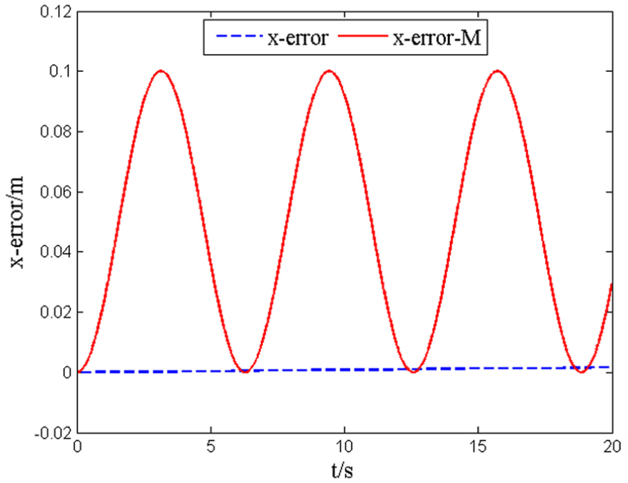
Comparison of x-error curves between modified numerical value and numerical value.

Figure 10.

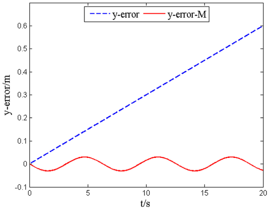
Comparison of y-error curves between modified numerical value and numerical value.

Figure 11.

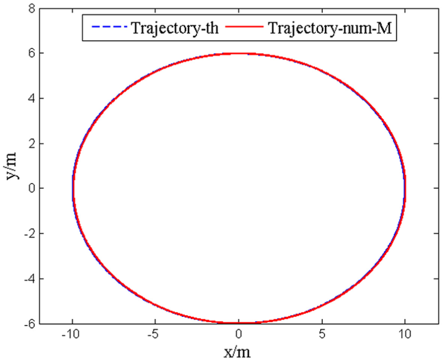
Comparison of trajectories between modified numerical value and theoretical value.

Figure 12.

Constraint torque curves.

Figure 13.

Driving torque curves generated by the motors.

Conclusion and future work

With the aim of dynamic modeling of the climbing robot with dual-cavity structure and wheeled locomotion mechanism, this study establishes the dynamic equation based on the Udwadia–Kalaba equation. The research process results in several conclusions as follows:

1. The trajectory constraint of the climbing robot is regarded as the external constraint of the system and integrated into the dynamic equation dexterously based on the idea of the Udwadia–Kalaba equation. The consideration of velocity-based constraint can reduce the error to guarantee that the trajectories obtained by modified numerical integration are close to the numerical trajectory as possible.

2. The driving torques required to guarantee the climbing robot to move along the given trajectory are obtained explicitly by solving Udwadia–Kalaba equation, which overcomes the disadvantage of obtaining dynamical equation from traditional Lagrange equation by Lagrange multiplier effectively.

3. The methodology described in this article can also be applied to many other kinds of climbing robots, such as climbing robots with magnetic adhesion or tracked type. In addition, the trajectory constraints are geometrical shapes of many kinds.

However, the simulation in this article is executed on the condition which the initial condition satisfies the constrained equation. Therefore, the future work is the dynamics modeling of climbing robot which the initial condition does not satisfy the constrained equation and the error reduction of the dynamic modeling by further study. Moreover, in numerous factors, the friction, no doubt, is one of the biggest nonlinear factors in the dynamic modeling of climbing robot. It requires in-depth discussion to obtain the precise model of the friction.