
Abstract
It is a common movement type in industrial production for the end-effector of industrial robot executing tasks according to desired track. High nonlinearity and coupling are shown from the dynamic characteristic of industrial robot because of the constrained relationship brought by desired task. Therefore, it is difficult to establish dynamical equation with traditional Lagrange equation. Aiming at the dynamics modeling of industrial robot subject to constraint, the additional torque and dynamical equation of industrial robot subject to some desired trajectory is acquired based on the famous Udwadia–Kalaba equation in analytical mechanics field. The simple approach overcomes the disadvantage of obtaining dynamical equation from traditional Lagrange equation by Lagrange multiplier. But the numerical results obtained by integrating the constrained dynamic equation yield the errors. A numerical algorithm is proposed to reduce the errors by modifying the derived dynamic equation. The simulation results prove that the modified algorithm can be more precisely utilized in dynamics modeling of industrial robot subject to constraint.
Introduction
For industrial robot, the accurate kinematic and dynamical models are the basis for completing all kinds of tasks. Compared with mature kinematic model, the dynamical model, especially the industrial robot whose end-effector moves according to desired track, shows high nonlinearity and coupling in its dynamic characteristic for the constrained relationship brought by desired track. Therefore, it is an important basis for realizing high-quality movement control to establish mathematical model which can describe dynamic characteristics of movement limitation system. At present, most of the scholars pay their attention to control algorithm of industrial robot, while few of them concern about the dynamical modeling problem. A constrained robotic system is a mechanical system, where we need to consider kinematic constraint conditions explicitly in dynamic modeling process. MH Korayem et al. 1 used the traditional Lagrange multiplier method to deal with dynamical modeling of mobile manipulator. The disadvantage of the Lagrange multiplier is relying on special approaches to the determination of the multipliers, and it is often very difficult to find the multipliers to obtain the explicit equations for systems that have large numbers of degrees of freedom and a series of non-integrable constraints. P Sanchez-Sanchez and MA Arteaga-Perez 2 proposed a simple method for obtaining the dynamic model of robot manipulators. But it is only beneficial to establish the dynamic equation for the unconstrained system. Kane 3 proposed a general method to obtain the dynamical system’s equation of motion which originated from Gibbs and Appell’s quasi-coordinates. Y-H Jia et al. 4 derived the equations of motion for the unconstrained planar dual-arm space robot using Kane’s equations. By inserting the constraint equations in terms of accelerations into the equations of motion for the unconstrained system, the reduced-order equations for the constrained system were obtained which contain only independent motion variables. Kane’s equation applies to holonomic constraints and also non-holonomic constraints and does not involve Lagrange multiplier. Computational complexity can be largely reduced for systems with a large number of degrees of freedom compared with Newtonian and Lagrange methods. Certainly, Kane’s method has its own disadvantage. It requires a suitable choice of problem-specific generalized speeds which relies on experience in a large part. SK Saha et al. 5 reviewed different methods on constrained multi-body dynamics formulations and summarized the advantages and disadvantages, respectively.
It is well known that it is impossible to create a new fundamental principle for the theory of motion and equilibrium of discrete, dynamical systems. However, as early as in 1996, Firdaus Udwadia of University of Southern California comes up with a multi-body dynamical modeling method that is Udwadia–Kalaba equation and obtains many research results. The Udwadia–Kalaba equation has been proposed that is useful to help us understand nature’s law from new points of view. The Udwadia–Kalaba equation describes the dynamics of constrained systems from Gauss’ principle. This method can establish system dynamical equations under holonomic constraint and non-holonomic constraint in a relatively simple way. Using this method, one can get analytical expression of constraint force without Lagrange multiplier.6–15 Unfortunately, in the hereafter 20 years until now, this method has not been paid too much attention, and its main application field focuses on dynamical modeling and control research of satellite system. It has seldom been used in robot field. Only J Huang et al. 16 used this method to build a parallel robot dynamical model, and H Zhao et al. 17 established the dynamical model of a machine fish.
The modeling process of the Udwadia–Kalaba equation has three steps. First, in terms of the generalized coordinates, the unconstrained dynamical system whose equations of motion can be written using traditional Lagrange method is considered. Then, the constraint equations are formed. In the end, the additional generalized forces of constraint are imposed on the system. That is to say, add the force resulted from the presence of constraints to the unconstrained system’s force.
In this article, the motion path of the end-effector is regarded as a constraint, and the dynamic equation is obtained based on the Udwadia–Kalaba equation. However, the results using numerical integration of the dynamic equations do not satisfy the constraint equations precisely. A modified approach is proposed to reduce the errors and obtain more precise constrained motion.
Udwadia–Kalaba equation
To industrial manipulator without constraint, the general form of its dynamical equation can be shown as

in which
The uncontrolled system is now subjected to the

These

in which

in which
in which
That is to say, the dynamical equation of constraint to multi-body mechanical system is shown in the following general form
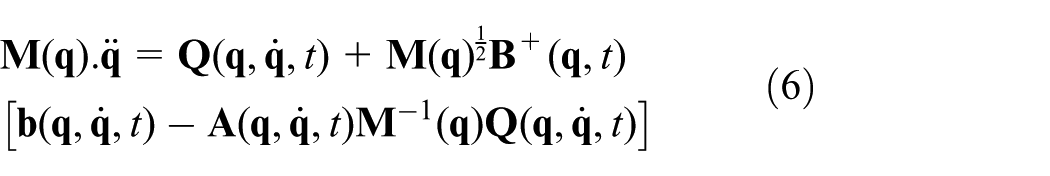
or

The standard Lagrange multiplier formulation of the problem of constrained motion can be shown as

in which


Now, substituting equation (8) into the practical acceleration level constraints (9), one can solve for the Lagrange multipliers by direct inversion

Substituting equation (10) into equation (8)

in which
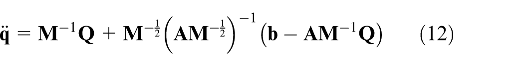
According to the matrix theory, for the matrices

So equation (12) has the same form as equation (6). There are two points to highlight:
It is impossible to create a new fundamental principle for the theory of dynamic modeling of the constraint systems. Even though the fundamental theory is completely different (The standard Lagrange multiplier formulation is based on D’Alembert’s principle, and the Udwadia–Kalaba equation is based on Gauss’ rule), the dynamic equations have the same form on the premise that the matrices
Comparing with the Lagrange multiplier formulation, Udwadia–Kalaba equation eliminates the computing complexity, which comes from the Lagrange multiplier, and enlarges the applied range of the dynamic modeling because of the application of the Moore–Penrose generalized inverse.
Dynamic modeling and simulation of the industrial robot subject to constraint
Dynamic modeling on manipulator without constraint
As shown in Figure 1, it is a schematic diagram of two-link robot manipulator moving on the vertical plane. The system generalized coordinate is

Sketch map of the two-link planar manipulator subject to constraint.
Let us establish the dynamical equation without constraint using Lagrange equation.
The total kinetic energy of system is

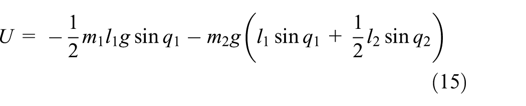
The potential energy of system is
The dynamical equation of the system can be acquired by Lagrange equation

in which


The dynamical equation of the system without constraint is shown as

in which

Because the system has not been constrained by now,
Then, we have

Dynamics modeling subject to constraint
The trajectory constraint of the end-effector is summarized as


in which


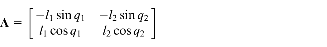
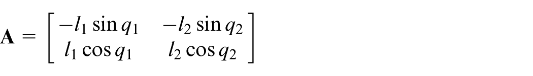
Differentiating equation (19) with respect to time twice


Differentiating equation (18) with respect to time twice


According to equations (20) and (21), one can have the following constraint equation

in which

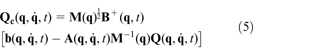
Then, the additional torques for system to satisfy the given trajectory is explicitly determined by equation (5) and is shown as

Finally, the dynamic equation is obtained by equations (4), (5), and (23)

Result and analysis to simulation
It is assumed that

Sketch map of the initial configuration of the two-link planar manipulator subject to constraint.
The theoretical curve of joint angles and joint angular velocities can be obtained by solving equation (19). It can be regarded as reference curve for the following study. Figure 3 represents the joint angles at each joint of the robotic system subjected to the constraints of the vertical plane while the end-effector stays at the initial position, in which the solid line represents the theoretical value and the dashed line represents the numerical integration value. It is obvious that the dashed line approximates the solid line. The first link moves from the initial configuration to 90° and then comes back to the initial position. The second link moves from the initial configuration to the horizontal position and then comes back to the initial position. So, the link’s movement is periodic which leads to the periodic moving of the end-effector from the lowest position to the highest position and then back to the lowest position. However, obvious errors between the solid line and the dashed line still exist. Figure 4 represents the errors between the solid line and the dashed line. It is observed that the errors gradually increase with time. Figure 5 represents the joint angular velocities. Figure 6 represents the angular velocities errors between the theoretical value and the numerical integration value. It is also observed that the errors gradually increase with time. But the trend is gentle than the joint angular errors. Thus, it is necessary to consider the numerical method for reducing the errors; this is handled in the following section.

Sketch map of the joint angles.

Errors of the joint angles.

Sketch map of the joint angular velocities.

Errors of the joint angular velocities.
Numerical method to reduce errors
It is well known that numerical integration scheme on the second-order differential equation needs a set of two first-order differential equations. The second-order differential equation of equation (6) is expressed as a set of the first-order differential equations as


However, it is found that the numerical results show unneglectable errors between the theoretical curve and the numerical integration curve as shown in the previous example. This is because the dynamic equation utilizes equation (3) and neglects the velocity-based constraint that differentiates the constraint equations once with respect to time. It can be written as

Then, the dynamic equation can be modified as


It is important to note that the new term
Differentiating equation (19) with respect to time once


According to equation (26), one can have the following constraint equation

in which

Substituting the dynamic equation of the unconstrained system and the constraint equations into equation (27), the dynamic responses and constraint forces can be obtained. Figure 7 represents the joint angles at each joint of the robotic system subjected to the constraints of the vertical plane depending on the modified numerical integration method, in which the solid line shows the theoretical curve and the dashed line shows the modified curve. Figure 8 represents the errors between the theoretical curve and the modified curve. It is observed that the errors’ growth trend is improved obviously and decreased by one order of magnitude. Figure 9 represents the joint angular velocities, in which the solid line shows the theoretical curve and the dashed line shows the modified curve. Figure 10 represents the errors between the theoretical curve and the modified curve. It is observed that the errors also decreased by one order of magnitude. Figure 11 compares the errors of the constraints depending on the application of the proposed numerical scheme, where Figure 11(a) and (c) represents the errors in the satisfaction of equation (19) and Figure 11(b) and (d) represents the errors in the first time derivative of equation (19). It is observed that the errors obtained by the numerical integration of equation (25) gradually increase with time to veer away from the constrained path. The proposed numerical scheme describes more precise dynamic responses; still, the errors do not perfectly disappear. Figure 12 represents the constraint torques to be required at each joint for its movement.
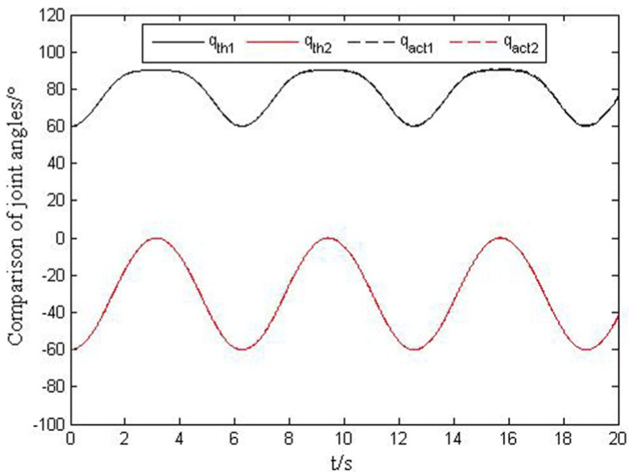
Sketch map of the joint angles depending on the modified numerical integration method.

Errors of the joint angles between the theoretical curve and modified curve.

Sketch map of the joint angular velocities depending on the modified numerical integration method.

Errors of the joint angular velocities between the theoretical curve and modified curve.
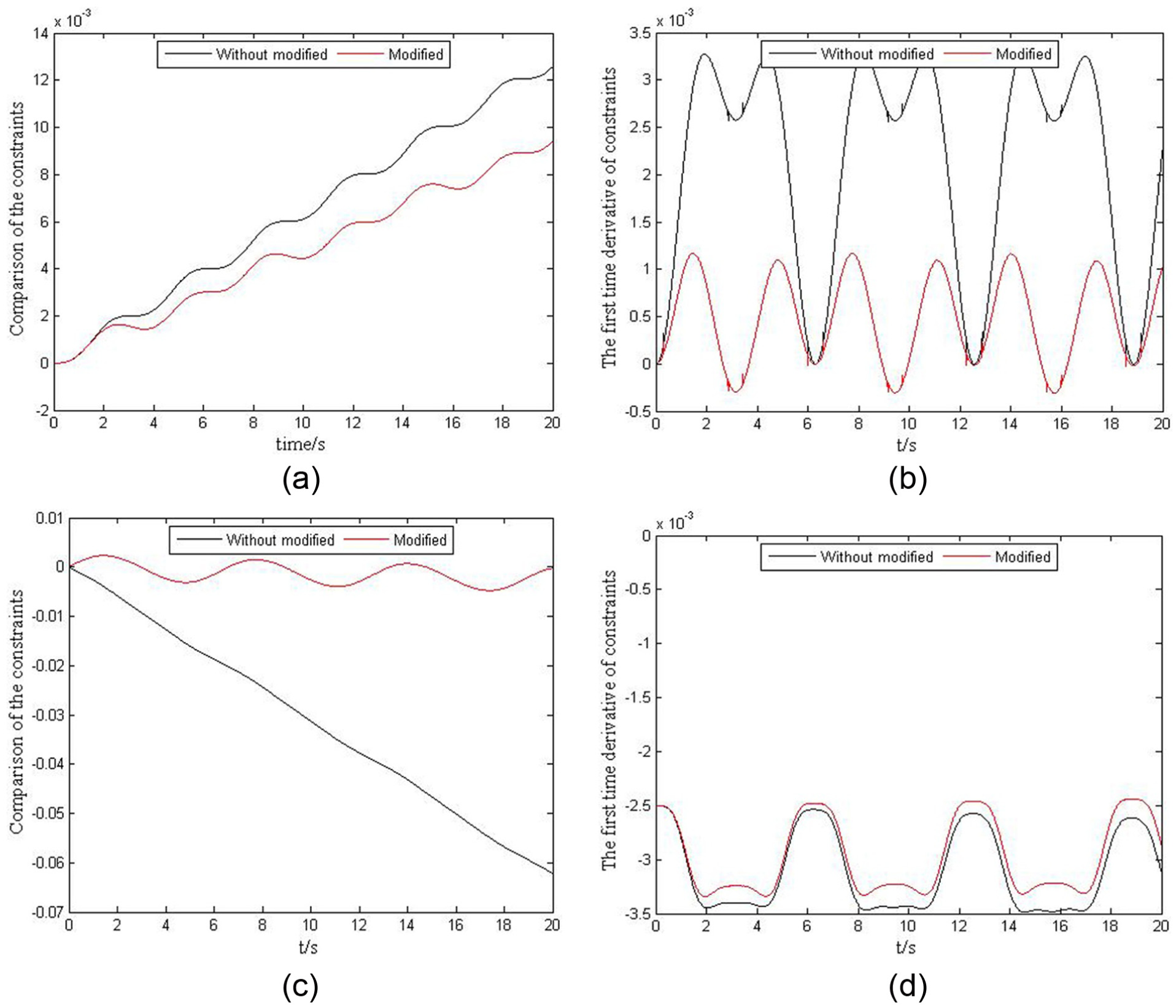
Errors of constraints: (a) constraint error of X direction, (b) the first time derivative of constraint error of X direction, (c) constraint error of Y direction, and (d) the first time derivative of constraint error of Y direction.

Sketch map of the joint torque.
Conclusion and future works
Aiming at the dynamics modeling of industrial robot subject to constraint, this article establishes the dynamic equation based on the Udwadia–Kalaba equation and proposes a modified algorithm to reduce the error caused by numerical integration. The research process reveals some conclusions as follows:
The geometric constraint and the trajectory of the end-effector are considered as the external constraint of the system, and the constrained relationship of the system is integrated into the dynamic equation dexterously based on the idea of the Udwadia–Kalaba equation. The simple method overcomes the disadvantage of obtaining dynamical equation from traditional Lagrange equation by Lagrange multiplier effectively.
The velocity-based constraint is considered in dynamics modeling process to reduce the error. The numerical simulation results prove that the dynamical equation established by this method decreases the joint angle and joint angular velocity errors by one order of magnitude and conforms to the matter of fact precisely.
Future work mainly consists of two tasks:
However, the simulation is executed on the condition which the initial condition satisfies the constrained equation, then the next research direction is the dynamics modeling of the industrial robot subject to constraint which the initial condition does not satisfy the constrained equation and expanding to the three-dimensional industrial robot.
The error is improved to a certain degree, but not perfect. So, the next research is to reduce the error by proper control strategy.
Footnotes
Academic Editor: Chuanzeng Zhang
Declaration of conflicting interests
The author(s) declared no potential conflicts of interest with respect to the research, authorship, and/or publication of this article.
Funding
The author(s) received no financial support for the research, authorship, and/or publication of this article.