Distributed parallel computing of the recursive eigenvalue search in the context of transfer matrix method for multibody systems

Abstract

The modeling and solving a transcendental eigenvalue problem are important issues in the transfer matrix method for linear multibody systems. Based on the recursive eigenvalue search algorithm for transfer matrix method for linear multibody system, the distributed parallel approach for assembling overall transfer matrix and searching eigenvalues is proposed. This is achieved based on Message Parallel Interface. The influence of the CPU core number as well as the distributed network environment on the final computational time is analyzed through numerical examples of both a non-uniform beam and a multiple launch rocket system. The results indicate that the computational time is significantly reduced by the proposed parallel computing method, so that the computational efficiency on optimization and design of complex multibody systems can be improved.

Introduction

The demand for multibody system dynamics (MSD) computation is increasing in various fields, such as vehicles, ships, aeronautics, and astronautics weapons, while the MSD models become more and more complicated. ¹ Typically, the solution of a complex multibody system will cost a plenty of time, thus the conventional static design pattern can hardly meet the requirement of dynamics design. In light of such concern, the computational speed needs to be accelerated. Although this can be achieved by raising the level of hardware, the computational speed of a single-core CPU is limited due to manufacturing process, ² thus resulting in the emergence of the multicore CPU handling a problem simultaneously. At the same time, the computer cluster system can be constructed using relatively inexpensive computers connected via the high-speed local area network (LAN), which is more cost-effective compared with supercomputers. ³ These provide the foundation for the software technology such as the parallelization of numerical algorithms. ⁴ To shorten the computing time, many commercial and open source dynamics software including ADAMS, ANSYS, MBDyn, and so on have introduced the idea of parallel computing. A lot of research work in parallel computing^4–9 is also investigated by scholars. D Negrut et al. ⁵ concentrated on the use of commodity parallel computing in many-body frictional-contact dynamics, fluid–solid interaction analysis, and proximity computation. F González et al. ⁶ evaluated two non-intrusive parallelization techniques for MSD, namely, parallel sparse linear equation solvers and OpenMP. OA Bauchau ⁷ used domain decomposition techniques to achieve parallel processing of finite element method for flexible multibody systems.

The transfer matrix method for multibody systems (MSTMM) is a rather novel method for MSD. Compared with ordinary dynamics methods, MSTMM has the following characteristics: no global dynamics equation of the system is required, low matrix order is involved, and fast computing speed and highly stylized programming are achieved. ¹⁰ Its basic idea is to (1) break up the whole system into several elements, (2) use a matrix representing the mechanical properties of each element, (3) assemble these matrices by applying the automatic deduction theorem of the overall transfer equation of multibody systems, ¹¹ and (4) solve the overall transfer equation of the system.

The solution of the overall transfer equation is one of a key technique in MSTMM. D Bestle et al. ¹² proposed a recursive eigenvalue search algorithm for the transfer matrix method for linear multibody systems (linear MSTMM). Although this algorithm has a linear convergence rate, as is the same with those strategies based on sign change, it can solve both real and complex eigenvalue problems of a system and even find double roots. Moreover, this algorithm is more competitive and efficient in choosing step size than other strategies based on sign change.

To further improve the computational efficiency, a parallel algorithm for assembling the overall transfer matrix as well as recursively searching the eigenvalue is proposed in this article, and the distributed parallel computing environment based on the Message Parallel Interface (MPI) is built. A damped non-uniform beam with complex eigenvalues and a multiple launch rocket system (MLRS) with real eigenvalues are taken as numerical examples to verify the proposed method. This article provides a feasible way to further improve the computational speed of linear MSTMM.

Basic idea of linear MSTMM

In the inertial coordinate system, r , $\mathbf{\theta }$ , m , and q are used to represent the linear displacement, angular displacement, internal moment, and internal force, respectively, of one point fixed on an element vibrating in space relative to its equilibrium position, where $\mathit{r}=[\begin{array}{ccc}x\hfill & y\hfill & z\hfill \end{array}{]}^{\mathrm{T}}$ , $\mathbf{\theta }=[\begin{array}{ccc}{\theta }_x\hfill & {\theta }_y\hfill & {\theta }_z\hfill \end{array}{]}^{\mathrm{T}}$ , $\mathit{m}=[\begin{array}{ccc}{m}_x\hfill & m_y\hfill & m_z\hfill \end{array}{]}^{\mathrm{T}}$ , and $\mathit{q}=[\begin{array}{ccc}{q}_x\hfill & q_y\hfill & q_z\hfill \end{array}{]}^{\mathrm{T}}$ . The state vector of the connection point is defined as $\mathit{z}=[\begin{array}{cccc}{\mathit{r}}^{\mathrm{T}}\hfill & {\mathbf{\theta }}^{\mathrm{T}}\hfill & {\mathit{m}}^{\mathrm{T}}\hfill & {\mathit{q}}^{\mathrm{T}}\hfill \end{array}{]}^{\mathrm{T}}$ under physical coordinates or $\mathit{Z}=[\begin{array}{cccc}{\mathit{R}}^{\mathrm{T}}\hfill & {\mathbf{\Theta }}^{\mathrm{T}}\hfill & {\mathit{M}}^{\mathrm{T}}\hfill & {\mathit{Q}}^{\mathrm{T}}\hfill \end{array}{]}^{\mathrm{T}}$ under modal coordinates by introducing modal transformation $\mathit{z}=\mathit{Z}{e}^{\mathrm{i}\omega t}$ , where $\mathit{R}=[\begin{array}{ccc}X\hfill & Y\hfill & Z\hfill \end{array}{]}^{\mathrm{T}}$ , $\mathbf{\Theta }=[\begin{array}{ccc}{\Theta }_x\hfill & {\Theta }_y\hfill & {\Theta }_z\hfill \end{array}{]}^{\mathrm{T}}$ , $\mathit{M}=[\begin{array}{ccc}{M}_x\hfill & M_y\hfill & M_z\hfill \end{array}{]}^{\mathrm{T}}$ , and $\mathit{Q}=[\begin{array}{ccc}{Q}_x\hfill & Q_y\hfill & Q_z\hfill \end{array}{]}^{\mathrm{T}}$ are the modal coordinates arrays corresponding to r , $\mathbf{\theta }$ , m , and q , and $\omega$ is the natural frequency. Here, ${\mathit{Z}}_{j,I}$ and ${\mathit{Z}}_{j,O}$ are used to represent the state vectors of the input end I and output end O on element j, respectively. ${\mathit{Z}}_{j,I}$ and ${\mathit{Z}}_{j,O}$ possess the relationship ${\mathit{Z}}_{j,O}={\mathit{U}}_j{\mathit{Z}}_{j,I}$ , where ${\mathit{U}}_j$ is the transfer matrix of element j. Specially, if the input or output end of an element j is a boundary end, the state vector will be denoted as ${\mathit{Z}}_{j,0}$ , where “0” represents the boundary. Rui et al. ¹⁰ provide a library for the transfer matrices for a variety of typical elements.

For clarity, an example with a one-degree-of-freedom (1-DOF) lumped mass connected with a rod is shown in Figure 1.

Figure 1.

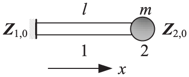
The 1-DOF system with a rod and a lumped mass.

The rod with length l and the lumped mass with mass m are numbered as 1 and 2, respectively. The state vector of the inner connection point between elements 1 and 2 is defined as ${\mathit{Z}}_{2,1}=[\begin{array}{cc}X\hfill & Q\hfill \end{array}{]}_{2,1}^{\mathrm{T}}$ , where X and Q denote the displacement and internal force related to this point. Analogously, the boundary state vector of the fixed end of the rod and the free end of the lumped mass are denoted as ${\mathit{Z}}_{1,0}=[\begin{array}{cc}0\hfill & Q\hfill \end{array}{]}_{1,0}^{\mathrm{T}}$ and ${\mathit{Z}}_{2,0}=[\begin{array}{cc}X\hfill & 0\hfill \end{array}{]}_{2,0}^{\mathrm{T}}$ , respectively, after taking the boundary condition into consideration. The transfer matrices of the rod and the lumped mass take the form ¹⁰

$$U_1=\left[\begin{array}{cc}\cos \beta l& -\frac{\sin \beta l}{\beta EA}\\ \beta EA\sin \beta l& \cos \beta l\end{array}\right],U_2=\left[\begin{array}{cc}1& 0\\ m{\omega }^2& 1\end{array}\right]$$

(1)

where $\beta =\sqrt{\rho {\omega }^2/E}$ , and $\rho$ , E, and A represent the density, Young’s modulus, and sectional area of the rod, respectively.

Then the transfer equation of the system can be obtained as

$${\mathit{Z}}_{2,0}={\mathit{U}}_2{\mathit{Z}}_{2,1}={\mathit{U}}_2{\mathit{U}}_1{\mathit{Z}}_{1,0}=:{\mathit{U}}_{\mathrm{all}}{\mathit{Z}}_{1,0}$$

(2)

where

$$U_{\mathrm{all}}=U_{\mathrm{2}}{U}_{\mathrm{1}}=\left[\begin{array}{cc}\cos \beta l& -\frac{\sin \beta l}{\beta EA}\\ m{\omega }^2\cos \beta l+\beta EA\sin \beta l& \cos \beta l-\frac{m{\omega }^2\sin \beta l}{\beta EA}\end{array}\right]$$

(3)

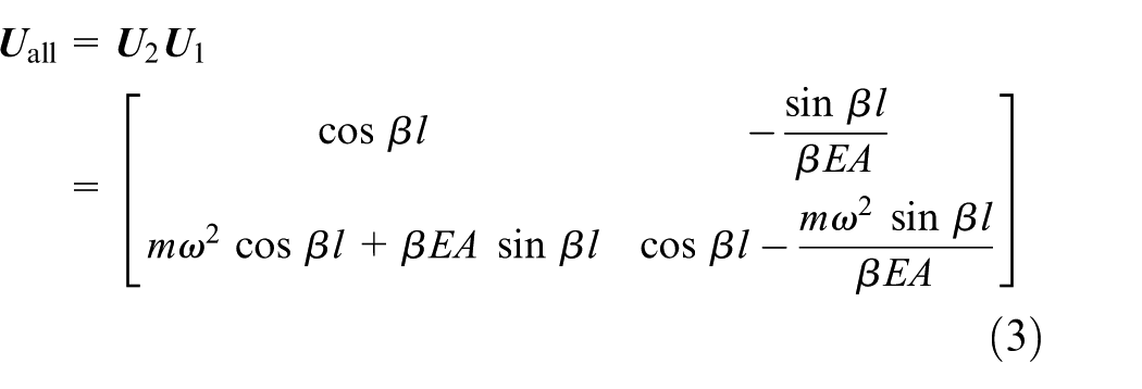
is the overall transfer matrix of the system.

The non-trivial solution of equation (2) leads to system characteristic equation as

$$\Delta (\omega )=\det {\overline{U}}_{\mathrm{all}}=\det U_{\mathrm{all}}(2,2)=\left|\cos \beta l-\frac{m{\omega }^2\sin \beta l}{\beta EA}\right|=0$$

(4)

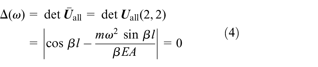
Then the eigenvalue $\omega$ of the system can be acquired by solving equation (4).

For a multibody system in a more generic topology, the overall transfer equation and the overall transfer matrix can be obtained by simply following the automatic deduction theorem of the overall transfer equation for multibody systems ¹¹ taking a general form

$${\mathit{U}}_{\mathrm{all}}{\mathit{Z}}_{\mathrm{all}}=0$$

(5)

where ${\mathit{Z}}_{\mathrm{all}}$ contains the state vectors of all the boundary points and cutting points and ${\mathit{U}}_{\mathrm{all}}$ is the overall transfer matrix of the system.

By eliminating zero elements corresponding to the known system boundary conditions in ${\mathit{Z}}_{\mathrm{all}}$ and removing the corresponding columns in ${\mathit{U}}_{\mathrm{all}}$ , equation (5) can be rewritten as

$${\overline{\mathit{U}}}_{\mathrm{all}}{\overline{\mathit{Z}}}_{\mathrm{all}}=0$$

(6)

where the coefficient matrix ${\overline{\mathit{U}}}_{\mathrm{all}}$ is a square matrix. For a given linear multibody system with determined dynamics parameters, the value of ${\overline{\mathit{U}}}_{\mathrm{all}}$ only depends on the vibration frequencies $\omega$ or complex numbers $s=-\delta \pm i\omega$ summarizing damping and frequency. To satisfy equation (6), the coefficient matrix ${\overline{\mathit{U}}}_{\mathrm{all}}$ needs to be singular resulting in the system characteristic equation as

$$\det {\overline{\mathit{U}}}_{\mathrm{all}}=0$$

(7)

The eigenvalues of a multibody system can be obtained by solving equation (7), which will be discussed in section “Recursive eigenvalue search algorithm.” It is worth mentioning that the order of the coefficient matrix ${\overline{\mathit{U}}}_{\mathrm{all}}$ is very low, which will not cost too much time in computation of determinant $\det {\overline{\mathit{U}}}_{\mathrm{all}}$ . From equation (4), it can also be found that the characteristic equation is a nonlinear or even transcendental function w.r.t. the eigenvalue. This indicates some popular eigensolvers, such as Lanczos, QR, and Arnoldi, cannot be applied in the context of linear MSTMM where the characteristic equation has no special structure.

Recursive eigenvalue search algorithm

For an undamped system, the solution of equation (7) can be achieved by searching the zeros of the equation $\Delta (\omega )=\det {\overline{\mathit{U}}}_{\mathrm{all}}$ , where $\omega$ is the real eigenvalues of the system. Common zero search strategy such as the bisection method is typically based on the sign change of $\Delta (\omega )$ , however, flawed to search double roots. And for a damped system, solving equation (7) indicates to solve $\Delta (s)=0$ , where $s=-\delta \pm i\omega$ is the complex eigenvalue. Therefore, solution of equation (7) changes to a two-dimensional variable problem $\Delta (\delta ,\omega )=0$ , which cannot be simply solved by search strategies based on sign change.

The basic idea of the recursive eigenvalue search algorithm for linear MSTMM is switching from zero search for $\Delta$ to minimization of its absolute value $\left|\Delta \right|$ , which is equally well applicable to both the real and the complex cases. It is much easier to recognize craters in $\left|\Delta \right|$ than sign changes in $\Delta$ as conical breaking-ins of $|\Delta (\omega )|$ or $|\Delta (s)|$ only happen in the neighborhood of singularities of the overall transfer matrix. ¹² Here, the real eigenvalue search is taken as an example to describe the basic process of this algorithm. For a one-dimensional variable continuous function $y=f(x)$ , x represents $\omega$ , and f represents $\left|\Delta \right|$ . N sample points $x_i(i=1,2,\dots ,N)$ are chosen on the search region $[x_1,x_N]$ of interest, and the corresponding function value $f(x_i)$ is denoted by $f_i(i=1,2,\dots ,N)$ . If $f_i<f_{i-1}$ and $f_i<f_{i+1}$ , there must be a local minimum in the interval $[x_{i-1},x_{i+1}]$ . All such intervals may be considered as interesting regions. Furthermore, N sample points on each region are chosen again for more detailed scanning to get more accurate local minimum. When the precision reaches the requirement, the resulting local minimum could be considered as the solution of $f(x)=0$ . During programming, the recursive method is used to achieve the above process, as it is named recursive eigenvalue search algorithm. Moreover, to ease the algorithm, and to reduce the comparison times while not missing the potential candidates, the local minimum condition is weakened as $f_i<f_{i-1}$ and $f_i\le f_{i+1}$ . The logical array L_i is defined as

$$L_i=\{\begin{array}{cc}1\hfill & f_i\le f_{i+1}\hfill \\ \multicolumn{1}{c}{0}& \mathrm{else}\hfill \end{array}$$

(8)

where 1 means true, while 0 means false. Consequently, the local minimum conditions $f_i<f_{i-1}$ and $f_i\le f_{i+1}$ can be rewritten as $M_i=\neg L_{i-1}\wedge L_i$ shown in Figure 2. There “¬” and “∧” means logical operation “NOT” and “AND,” respectively.

Figure 2.

Logical arrays of minimization strategy.

For each iteration in the one-dimensional minimum search in Bestle et al., ¹² a user-defined resolution $\epsilon$ corresponds to the necessary number $N_{\epsilon }$ of sample points required for an interval of interest, whereas the user-provided sample size N is used on such region of interest. The iteration will terminate if $N_{\epsilon }$ on this region of interest is no greater than N, indicating that resolution $\epsilon$ is achieved within this iteration. The algorithm recursively sweeps through all regions with potential minima till all local minima are found. As for two-dimensional minimum search, the scanning is done on a regular grid and the function comparison is evaluated in both the x- and y-directions. In correspondence, the user may provide different sampling numbers $N_x$ , $N_y$ and precision tolerances dx, dy in two search directions, and the algorithm stops only if both resolutions are achieved.

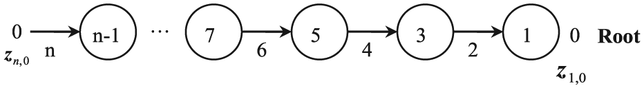
As discussed in the preceding section, the recursive eigenvalue search algorithm is more competitive in choosing step size than some strategies based on sign change. The following numerical example will provide some insights. If the number of rods and lumped masses in Figure 1 increases to 10, respectively, the system will become as shown in Figure 3, where the masses of the lumped masses are denoted as $m_2,m_4,\dots ,m_{20}$ .

Figure 3.

The 1-DOF system with 10 rods and 10 lumped masses.

The overall transfer equation of the system can be obtained as

$${\mathit{Z}}_{20,0}={\mathit{U}}_{20}{\mathit{U}}_{19},\dots ,{\mathit{U}}_2{\mathit{U}}_1{\mathit{Z}}_{1,0}={\mathit{U}}_{\mathrm{all}}{\mathit{Z}}_{1,0}$$

(9)

with the characteristic equation

$$\Delta (\omega )=det{\overline{\mathit{U}}}_{\mathrm{all}}=det{\mathit{U}}_{\mathrm{all}}(2,2)=0$$

(10)

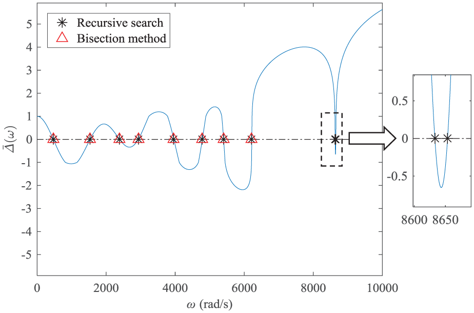
The variation trend of $\Delta (\omega )$ w.r.t. $\omega$ is shown in Figure 4 for aluminum rods with $\rho =2700\mathrm{kg}/{\mathrm{m}}^3$ , $E=0.69\times {10}^{11}\mathrm{N}/{\mathrm{m}}^2$ , $l=1\mathrm{m}$ , $A={10}^{-4}{\mathrm{m}}^2$ , and the lumped masses being $m_2=m_4=\cdots m_{20}=0.1\mathrm{kg}$ , respectively. The following transformation is made when the figure is plotted

$$\overline{\Delta }(\omega )=\{\begin{array}{cc}\Delta (\omega )\hfill & \mathrm{for}|\Delta (\omega )|\le 1\hfill \\ \multicolumn{1}{c}{\mathrm{sign}[\Delta (\omega )][1+{\log }_{10}|\Delta (\omega )|]}& \mathrm{for}|\Delta (\omega )|>1\hfill \end{array}$$

(11)

Figure 4.

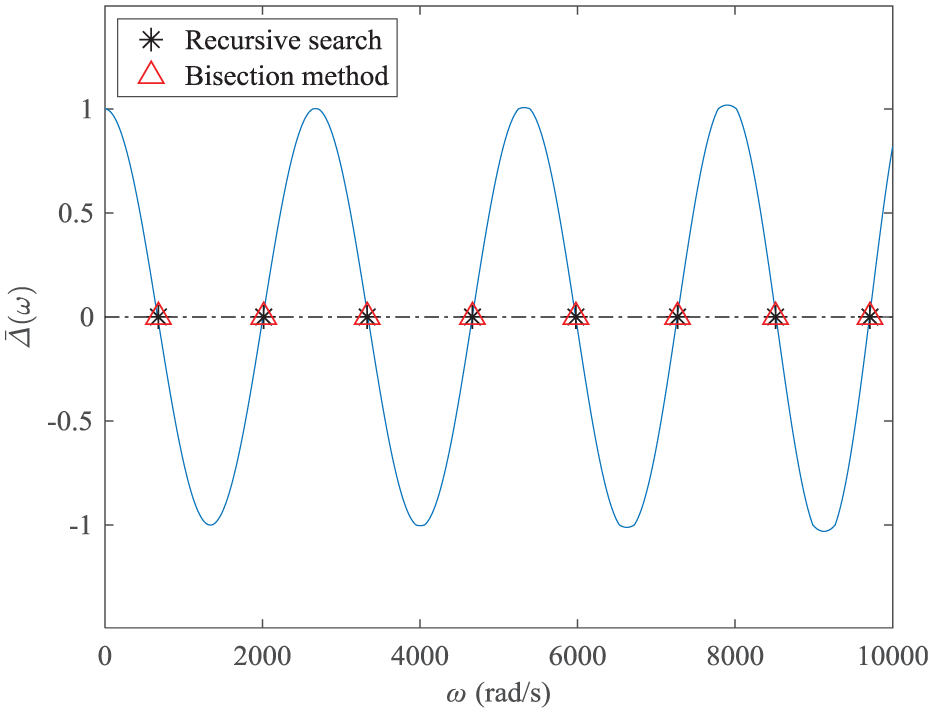
Variation in $\overline{\Delta }(\omega )$ w.r.t. $\omega$ with same lumped masses.

If one sets the sampling size $N=50$ and the absolute resolution $\epsilon ={10}^{-6}$ on the region $[0,{10}^4]$ , the eigenvalues of the system will be captured by both recursive eigenvalue search algorithm and the bisection method as depicted in Figure 4, where zeros are well distributed and isolated with a clear sign change. In this case, both methods work well.

If the lumped masses become different from each other with different mass values shown in Table 1, the variation trend of $\Delta (\omega )$ w.r.t. $\omega$ will become as shown in Figure 5, where there exists two roots in a narrow region. This makes the search algorithm based on sign change fail to find these roots without a high amount of enumeration effort. In contrast, the recursive eigenvalue search algorithm still works well with the same sampling size $N=50$ , which proves that the recursive search algorithm has good robustness in choosing sample points.

Table 1.

Values of lumped masses.

Lumped masses	m 2	m 4	m 6	m 8	m 10	m 12	m 14	m 16	m 18	m 20
Mass (kg)	0.25	0.093	0.55	1.00	0.50	0.50	0.60	0.15	0.15	1.00

Figure 5.

Variation in $\overline{\Delta }(\omega )$ w.r.t. $\omega$ with different lumped masses.

Principle and realization of distributed parallel computing technique

The basic idea of parallel computing is to separate a task into several parts and every part is solved by an individual processor parallel to reduce the computational time. ⁴ Furthermore, the distributed parallel computing technique not only divides the problem into parts but also assigns tasks to multiple computers interconnected by network so that the computers solve the tasks simultaneously. Then each computer uploads the results to the host to get a final result. ¹³

Construction of distributed parallel computing environment

As shown in Figure 6, to construct an MPI distributed parallel environment is to connect computers to the same LAN via Ethernet switches or other network equipment. In this article, four computers connected by a 100 Mb/s Ethernet switch are used to set up the distributed parallel computing environment. Each computer has an i7 quad-core processor with the frequency of 3.06 GHz. The parallel software used is MPICH2.

Figure 6.

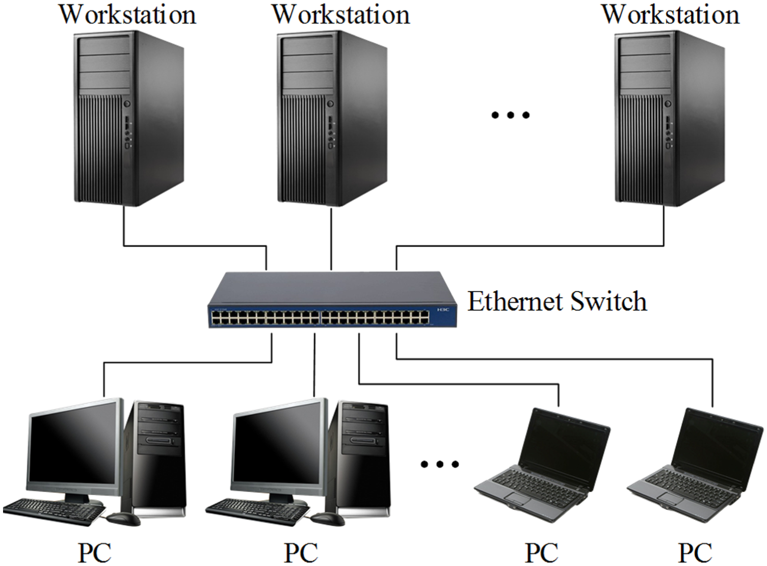
Distributed parallel computing environment.

Parallel computing algorithm for linear MSTMM

The master–slave mode is used as task allocation mechanism in this article. The master process is mainly responsible for the global division of tasks, which sends tasks to the slave processes and receives the results from the slaves. Meanwhile, the slave processes are responsible for computing the tasks assigned by the master process and returning the computational results to the master process. The major task of the eigenvalue computation using linear MSTMM is to assemble the overall transfer matrix and solving the characteristic equation. Thereby, the parallel algorithms can be designed in these two aspects.

Parallel computing algorithm for assembling the overall transfer matrix

Based on the automatic deduction theorem of the overall transfer equation of multibody systems, the assembly of the overall transfer matrix is a reassembling process after multiplying transfer matrices of each element in proper sequence according to the system topology.

As a chain system shown in Figure 7, the overall transfer matrix can be written as ${\mathit{Z}}_{1,0}=\mathit{Z}{\mathit{U}}_{\mathrm{all}}{\mathit{Z}}_{n,0}$ , where ${\mathit{U}}_{\mathrm{all}}={\mathit{U}}_1{\mathit{U}}_2{\mathit{U}}_3\dots {\mathit{U}}_n$ . The successive multiplication of n matrices can be distributed to m processes concurrently, including one master process numbered as 0 and m − 1 slave processes numbered from 1 to m − 1. As shown in Table 2, the multiplication of the first p (p = ceil(n/m)) matrices is allocated to the master process 0. In a similar manner, the multiplications of each follow-up p matrices are allocated to the slave processes from 1 to m − 2, respectively. Eventually, the remaining multiplications of n − (m − 1)p matrices are allocated to the last slave process m − 1. The slave processes send each computing result ${\overline{\mathit{U}}}_i(i=1,2,\dots ,m-1)$ to the master process. Then, the overall transfer matrix ${\mathit{U}}_{\mathrm{all}}={\overline{\mathit{U}}}_0{\overline{\mathit{U}}}_1\dots {\overline{\mathit{U}}}_{m-1}$ can be obtained by the master process.

Figure 7.

Topology figure of a chain system.

Table 2.

Matrix multiplication assignment.

Process	Assignment
Master (process 0)	${\overline{\mathit{U}}}_0={\mathit{U}}_1\dots {\mathit{U}}_p$
Slave (process 1)	${\overline{\mathit{U}}}_1={\mathit{U}}_{p+1}\dots {\mathit{U}}_{2p}$
…	…
Slave (process m − 2)	${\overline{\mathit{U}}}_{m-2}={\mathit{U}}_{(m-2)p+1}\dots {\mathit{U}}_{(m-1)p}$
Slave (process m − 1)	${\overline{\mathit{U}}}_{m-1}={\mathit{U}}_{(m-1)p+1}\dots {\mathit{U}}_n$

Multibody systems with general topology could eventually be treated as a tree system. Taking a tree system as an example shown in Figure 8, the overall transfer equation can be obtained as ${\mathit{U}}_{\mathrm{all}}{\mathit{Z}}_{\mathrm{all}}=0$ , where

$${\mathit{U}}_{\mathrm{all}}=\left[\begin{array}{ccccc}-\mathit{I}& {\mathit{T}}_{1-18}& {\mathit{T}}_{2-18}& {\mathit{T}}_{3-18}& {\mathit{T}}_{4-18}\\ \mathit{O}& {\mathit{G}}_{1-9}& {\mathit{G}}_{2-9}& \mathit{O}& \mathit{O}\\ \mathit{O}& \mathit{O}& \mathit{O}& {\mathit{G}}_{3-10}& {\mathit{G}}_{4-10}\\ \mathit{O}& {\mathit{G}}_{1-15}& {\mathit{G}}_{2-15}& {\mathit{G}}_{3-15}& {\mathit{G}}_{4-15}\end{array}\right],{\mathit{Z}}_{\mathrm{all}}=\left[\begin{array}{c}{\mathit{Z}}_{18,0}\\ {\mathit{Z}}_{1,0}\\ {\mathit{Z}}_{2,0}\\ {\mathit{Z}}_{3,0}\\ {\mathit{Z}}_{4,0}\end{array}\right]$$

(12)

$$\{\begin{array}{c}{\mathit{T}}_{1-18}={\mathit{U}}_{18}{\mathit{U}}_{17}{\mathit{U}}_{16}{\mathit{U}}_{15}{\mathit{U}}_{13}{\mathit{U}}_{12}{\mathit{U}}_{11}{\mathit{U}}_9{\mathit{U}}_5{\mathit{U}}_1\hfill \\ \multicolumn{1}{c}{{\mathit{T}}_{2-18}={\mathit{U}}_{18}{\mathit{U}}_{17}{\mathit{U}}_{16}{\mathit{U}}_{15}{\mathit{U}}_{13}{\mathit{U}}_{12}{\mathit{U}}_{11}{\mathit{U}}_{9,6}{\mathit{U}}_6{\mathit{U}}_2}\\ \multicolumn{1}{c}{{\mathit{T}}_{3-18}={\mathit{U}}_{18}{\mathit{U}}_{17}{\mathit{U}}_{16}{\mathit{U}}_{15,14}{\mathit{U}}_{14}{\mathit{U}}_{10}{\mathit{U}}_7{\mathit{U}}_3}\\ \multicolumn{1}{c}{{\mathit{T}}_{4-18}={\mathit{U}}_{18}{\mathit{U}}_{17}{\mathit{U}}_{16}{\mathit{U}}_{15,14}{\mathit{U}}_{14}{\mathit{U}}_{10,8}{\mathit{U}}_8{\mathit{U}}_4}\end{array}$$

(13)

$$\begin{array}{c}\{\begin{array}{c}{\mathit{G}}_{1-9}=-{\mathit{H}}_9{\mathit{U}}_5{\mathit{U}}_1\hfill \\ \multicolumn{1}{c}{{\mathit{G}}_{2-9}={\mathit{H}}_{9,6}{\mathit{U}}_6{\mathit{U}}_2}\end{array}\hfill \\ \{\begin{array}{c}{\mathit{G}}_{3-10}=-{\mathit{H}}_{10}{\mathit{U}}_7{\mathit{U}}_3\hfill \\ \multicolumn{1}{c}{{\mathit{G}}_{4-10}={\mathit{H}}_{10,8}{\mathit{U}}_8{\mathit{U}}_4}\end{array}\hfill \end{array},\{\begin{array}{c}{\mathit{G}}_{1-15}=-{\mathit{H}}_{15}{\mathit{U}}_{13}{\mathit{U}}_{12}{\mathit{U}}_{11}{\mathit{U}}_9{\mathit{U}}_5{\mathit{U}}_1\hfill \\ \multicolumn{1}{c}{{\mathit{G}}_{2-15}=-{\mathit{H}}_{15}{\mathit{U}}_{13}{\mathit{U}}_{12}{\mathit{U}}_{11}{\mathit{U}}_{9,6}{\mathit{U}}_6{\mathit{U}}_2}\\ \multicolumn{1}{c}{{\mathit{G}}_{3-15}={\mathit{H}}_{15,14}{\mathit{U}}_{14}{\mathit{U}}_{10}{\mathit{U}}_7{\mathit{U}}_3}\\ \multicolumn{1}{c}{{\mathit{G}}_{4-15}={\mathit{H}}_{15,14}{\mathit{U}}_{14}{\mathit{U}}_{10,8}{\mathit{U}}_8{\mathit{U}}_4}\end{array}$$

(14)

Figure 8.

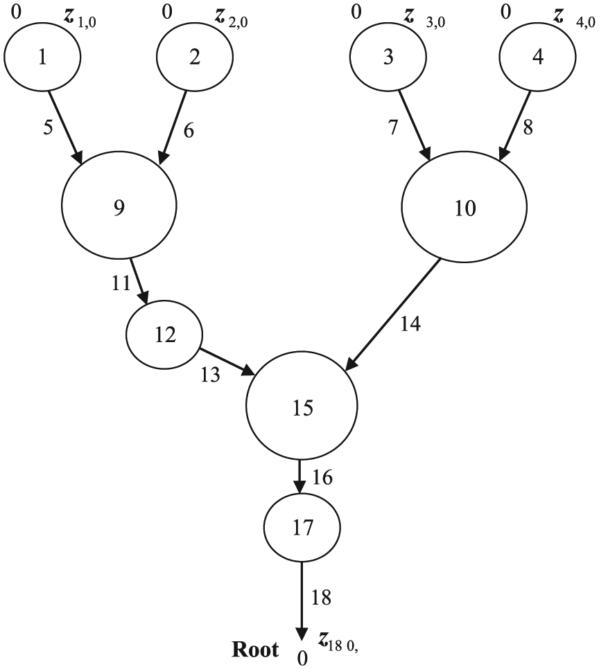
Topology figure of a tree system.

The detailed meaning of the above symbols can be found in Rui et al. ¹¹ As shown in equations (12)–(14), the overall transfer matrix ${\mathit{U}}_{\mathrm{all}}$ can be obtained by computing n sub-matrices T and G , which could be generally denoted by ${\mathit{M}}_i(i=1,2,\dots ,n)$ . ${\mathit{M}}_i$ can be allocated to m processes concurrently. For one master process and m − 1 slave processes, the matrix multiplication assignment is shown in Table 3. The master process and each of the first m − 2 slave processes have to compute p (p = ceil(n/m)) matrices, respectively. At the same time, the remaining n − (m − 1)p matrices are assigned to the last slave process m − 1. Finally, the slave processes send each computing result to the master process, and then the master process assembles ${\mathit{U}}_{\mathrm{all}}$ to obtain the overall transfer matrix.

Table 3.

Matrix computation assignment.

Process	Assignment
Master (process 0)	${\mathit{M}}_i(i=1,\dots ,p)$
Slave (process 1)	${\mathit{M}}_i(i=p+1,\dots ,2p)$
…	…
Slave (process m − 2)	${\mathit{M}}_i(i=(m-2)p+1,\dots ,(m-1)p)$
Slave (process m − 1)	${\mathit{M}}_i(i=(m-1)p+1,\dots ,n)$

Parallel recursive eigenvalue search algorithm

The first step of the eigenvalue search algorithm is to compute the function value $f(x_i)(i=1,2,\dots ,N)$ on the N sample points $x_i$ on the region $[x_1,x_N]$ . This step can be parallelized first. Function evaluations $f(x_i)$ can be allocated to m processes in parallel. As shown in Table 4, every p (p = ceil(N/m)) sample points are assigned to master process 0 and slave processes 1∼m − 2 to compute, respectively. And N − (m − 1)p sample points are assigned to the slave process m − 1.

Table 4.

Function value computation assignments.

Process	Assignment
Master (process 0)	$f(x_i)(i=1,\dots ,p)$
Slave (process 1)	$f(x_i)(i=p+1,\dots ,2p)$
…	…
Slave (process m − 2)	$f(x_i)(i=(m-2)p+1,\dots ,(m-1)p)$
Slave (process m − 1)	$f(x_i)(i=(m-1)p+1,\dots ,N)$

After the slave processes return each function value $f(x_i)$ to the master process, the master process is then able to compute the local minima on the region $[x_1,x_N]$ according to the algorithm given in section “Recursive eigenvalue search algorithm.”

Assuming there are k local minima $f_j(x_i)(j=1,\dots ,k)$ and the corresponding subintervals are $[x_{i-1},x_{i+1}{]}_j(j=1,\dots ,k)$ , the final result can be obtained by further iterations on these k subintervals till the required accuracy. The computation on these k subintervals is independent from each other and can also be performed in parallel. These k subintervals can be allocated to m processes. As shown in Table 5, each p (p = ceil(k/m)) subintervals are assigned to the master process 0 and slave processes 1∼m − 2, respectively. And the remaining k − (m − 1)p subintervals are assigned to the slave process m − 1.

Table 5.

Assignments of subintervals.

Process	Assignment
Master (process 0)	$[x_{i-1},x_{i+1}{]}_j(j=1,\dots ,p)$
Slave (process 1)	$[x_{i-1},x_{i+1}{]}_j(j=p+1,\dots ,2p)$
…	…
Slave (process m − 2)	$[x_{i-1},x_{i+1}{]}_j(j=(m-2)p+1,\dots ,(m-1)p)$
Slave (process m − 1)	$[x_{i-1},x_{i+1}{]}_j(j=(m-1)p+1,\dots ,k)$

The whole process of the eigenvalue search is shown in Figure 9.

Figure 9.

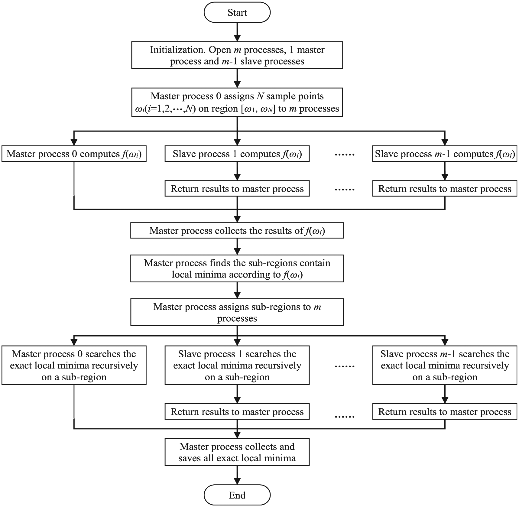
Flowchart of parallel eigenvalue search.

Example of a non-uniform beam

Figure 10(a) shows a non-uniform beam with length L. More detailed geometry parameters of the cross section are marked in Figure 10(a). The cross-sectional area is A(x), and the sectional moment of inertia is I(x), where

$$A(x)=A_0{\chi }^2,I(x)=I_0{\chi }^4$$

(15)

A ₀ and I₀ are the cross-sectional area and the sectional moment of inertia at x = 0, respectively, and $\chi =x(\alpha -1)/L+1$ and $\alpha =b_L/b_0=h_L/h_0$ .

Figure 10.

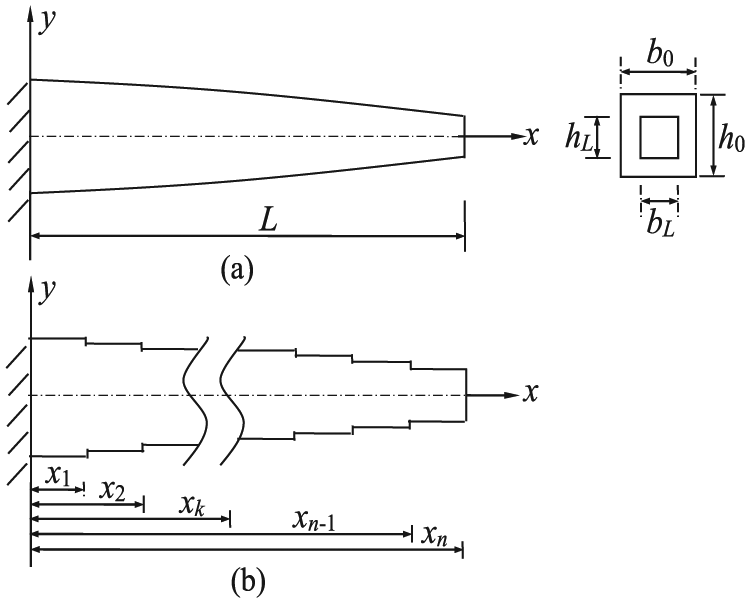
Non-uniform beam model.

The non-uniform beam can be discretized into n segments of uniform beam elements with length $l=L/n$ and height $h_k={\alpha }_k{h}_0(k=1,2,\dots ,n)$ shown in Figure 10(b), where ${\alpha }_k=(\alpha -1)k/n+1$ . The total volume of the beam segments from 1 to k is $V_k=A_0{L}_k({\alpha }_k^2+{\alpha }_k+1)/3$ , where $L_k=\mathrm{kL}/n$ is the length of the corresponding beam segments. Therefore, the equivalent volume of each uniform beam element is $V_k^e=V_k-V_{k-1}$ , the equivalent cross-sectional area is $A_k^e=V_k^e/l$ , and the equivalent sectional moment of inertia is $I_k^e=I_0(\sqrt{A_k^e/A_0}{)}^4$ .

Taking the uniform beam segment as a Euler–Bernoulli beam with free and damped transverse vibration, its dynamics equation can be obtained as ¹⁴

$$\overline{m}\frac{{\partial }^{2}y}{\partial t^2}+\eta \frac{\partial y}{\partial t}+\mathrm{EI}\frac{{\partial }^{4}y}{\partial x^4}=0$$

(16)

where $\overline{m}=\rho A$ is the line mass density, and $\rho$ , A, $\eta$ , E, and I are the density, cross-sectional area, damping coefficient, Young’s modulus, and sectional moment of inertia, respectively.

By applying linear MSTMM, the transfer matrix of the beam can be obtained as

$$\mathit{U}=\left[\begin{array}{cccc}S(\lambda l)\hfill & \frac{T(\lambda l)}{\lambda }\hfill & \frac{U(\lambda l)}{\mathrm{EI}{\lambda }^2}\hfill & \frac{V(\lambda l)}{\mathrm{EI}{\lambda }^3}\hfill \\ \multicolumn{1}{c}{\lambda V(\lambda l)}& S(\lambda l)\hfill & \frac{T(\lambda l)}{\mathrm{EI}\lambda }\hfill & \frac{U(\lambda l)}{\mathrm{EI}{\lambda }^2}\hfill \\ \multicolumn{1}{c}{\mathrm{EI}{\lambda }^{2}U(\lambda l)}& \mathrm{EI}\lambda V(\lambda l)\hfill & S(\lambda l)\hfill & \frac{T(\lambda l)}{\lambda }\hfill \\ \multicolumn{1}{c}{\mathrm{EI}{\lambda }^{3}T(\lambda l)}& \mathrm{EI}{\lambda }^{2}U(\lambda l)\hfill & \lambda V(\lambda l)\hfill & S(\lambda l)\hfill \end{array}\right]$$

(17)

where $\lambda =\sqrt[4]{((-(\overline{m}{s}^2+\eta s))/(\mathrm{EI}))}$ , and $S(x)$ , $T(x)$ , $U(x)$ , and $V(x)$ are the Крылов functions

$$\{\begin{array}{c}S(x)=\frac{\cosh x+\cos x}{2},T(x)=\frac{\sinh x+\sin x}{2}\hfill \\ \multicolumn{1}{c}{U(x)=\frac{\cosh x-\cos x}{2},V(x)=\frac{\sinh x-\sin x}{2}}\end{array}$$

(18)

If each beam segment from left to right is numbered as 1 to n, respectively, and the transfer direction is defined from left to right, then the overall transfer equation of the non-uniform beam can be acquired as

$${\mathit{Z}}_{n,0}={\mathit{U}}_n{\mathit{U}}_{n-1}\dots {\mathit{U}}_1{\mathit{Z}}_{1,0}={\mathit{U}}_{\mathrm{all}}{\mathit{Z}}_{1,0}$$

(19)

where ${\mathit{Z}}_{1,0}$ and ${\mathit{Z}}_{n,0}$ are the boundary state vectors at the leftmost and rightmost sides of the beam, respectively, and ${\mathit{U}}_i(i=1,2,\dots ,n)$ is the transfer matrix of each beam segment, and

$${\mathit{U}}_{\mathrm{all}}=\left[\begin{array}{cccc}{u}_{11}\hfill & u_{12}\hfill & u_{13}\hfill & u_{14}\hfill \\ \multicolumn{1}{c}{u_{21}}& u_{22}\hfill & u_{23}\hfill & u_{24}\hfill \\ \multicolumn{1}{c}{u_{31}}& u_{32}\hfill & u_{33}\hfill & u_{34}\hfill \\ \multicolumn{1}{c}{u_{41}}& u_{42}\hfill & u_{43}\hfill & u_{44}\hfill \end{array}\right]$$

(20)

is the overall transfer matrix of the system with the matrix element $u_{\mathrm{ij}}(i=1,2,3,4;j=1,2,3,4)$ .

By substituting the boundary conditions ${\mathit{Z}}_{n,0}=[\begin{array}{cccc}Y\hfill & {\Theta }_z\hfill & 0\hfill & 0\hfill \end{array}{]}_{n,0}^{\mathrm{T}}$ and ${\mathit{Z}}_{1,0}=[\begin{array}{cccc}0\hfill & 0\hfill & M_z\hfill & Q_y\hfill \end{array}{]}_{1,0}^{\mathrm{T}}$ into equation (19), the characteristic equation could be obtained by

$$\Delta (s)=\left|\begin{array}{cc}{u}_{33}\hfill & u_{34}\hfill \\ \multicolumn{1}{c}{u_{43}}& u_{44}\hfill \end{array}\right|=0$$

(21)

where $s=-\delta +i\omega$ is the complex variable.

The proposed method can be applied to solve equation (21). The search accuracy is set to be 10⁻⁴, and the dynamics parameters are given as follows: L = 4 m, b₀ = 0.04 m, h₀ = 0.04 m, b_L = 0.02 m, h_L = 0.02 m, ρ = 2730 kg/m³, I₀ = 2.133 × 10⁻⁷ m⁴, E = 6.9 × 10¹⁰ Pa, and $\eta =40\mathrm{kg}/(\mathrm{ms})$ . Figure 11 shows the three-dimensional (3D) plot of ${\log }_{10}|\Delta (s)|$ with the number of segments n = 50. Table 6 shows the computational results of eigenvalue by MSTMM, which is the same as those obtained by direct variable separation method (DVSM) similar to Joshi. ¹⁵ The computational time by a single process of MSTMM and DVSM with different numbers of segments is shown in Figure 12, where MSTMM certainly costs less computational time that increases linearly with the number of segments.

Figure 11.

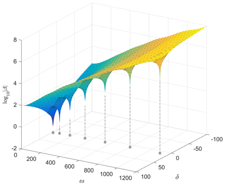
The eigenvalues log₁₀|Δ(s)| of non-uniform beam.

Table 6.

Comparison of the computational results of eigenvalue between MSTMM and DVSM.

Modal order	$-\delta +\mathrm{i}\omega$ (MSTMM)	$-\delta +\mathrm{i}\omega$ (DVSM)
1	−13.1872 + 10.4693i	−13.1872 + 10.4693i
2	−10.6857 + 69.8781i	−10.6857 + 69.8781i
3	−10.0808 + 175.8220i	−10.0808 + 175.8220i
4	−9.8454 + 332.8125i	−9.8454 + 332.8125i
5	−9.7312 + 541.7148i	−9.7312 + 541.7148i
6	−9.6679 + 802.6656i	−9.6679 + 802.6656i
7	−9.6294 + 1115.7216i	−9.6294 + 1115.7216i

MSTMM: transfer matrix method for multibody systems; DVSM: direct variable separation method.

Figure 12.

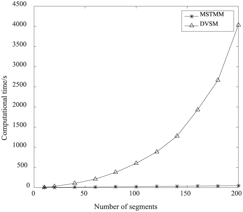
Comparison of computational time.

Typically, there are three indexes to describe the computational efficiency of parallel computing: computational time t, speedup ratio S_p, and parallel efficiency F_p, where S_p is defined as the ratio of the computational time with a single process (T₁) to that with p processes (T_p), namely, S_p = T₁/T_p and F_p = S_p/p. For a number of segments n = 100, the three indexes obtained by applying the proposed distributed parallel computing algorithm are listed in Table 7. Obviously, the parallel computing can accelerate the computational speed. From scheme no. 2–5 in Table 7, it is known that the computational speed of one PC with dual-core is slightly faster than two PCs with single-core; meanwhile, one PC with quad-core is slightly faster than four PCs all with single-core. This indicates that network delay has an impact on distributed parallel computing. Therefore, good network transmission speed should be ensured when using distributed parallel computing technique. Figure 13 shows how these indexes vary with CPU core numbers. Furthermore, with the increasing number of CPU cores, the computational time t is on the decline, but the trend is leveling off; meanwhile, the S_p increases and F_p decreases. This may be attributed to the increase in the communication overhead between different processes. Although the computation amount of a single process decreases since the number of CPU cores increases, the proportion of communication overhead relative to the computation amount for each process will increase, leading to the decrease in computational efficiency. To clarify, the computation scale is reduced by cutting down the number of segments of the beam to three and reducing the size of sample points. This will result in the preceding three indexes shown in Figure 14 and the proportion of average communication time t_c of each process to computational time t shown in Figure 15, respectively, where t_c only contains the time for each process to receive and send data using the MPI functions MPI_RECV, MPI_SEND, and MPI_BARRIER. From Figures 14 and 15, it can be found that S_p increases slowly and F_p becomes very low when the number of CPU cores rises. This is because the proportion of the communication time relative to the computational time enlarges and cannot be ignored. Under these circumstances, it has less effect to simply increase the number of CPU cores for improving the computational efficiency.

Table 7.

Parallel computational time, speedup ratio, and parallel efficiency.

Scheme no.	Number of process	Computational time t (s)	Speedup ratio Sp	Parallel efficiency Fp
1	1 (Single PC)	20.8462	1.0000	1.0000
2	2 (Single PC)	10.4343	1.9978	0.9989
3	4 (Single PC)	5.2757	3.9514	0.9878
4	1 + 1 (Distributed)	10.4576	1.9934	0.9967
5	1 + 1 + 1 + 1 (Distributed)	5.3131	3.9235	0.9809
6	2 + 2 + 2 + 2 (Distributed)	3.0752	6.7787	0.8473
7	3 + 3 + 3 + 3 (Distributed)	2.3135	9.0106	0.7509
8	4 + 4 + 4 +4 (Distributed)	1.7736	11.7537	0.7346

Figure 13.

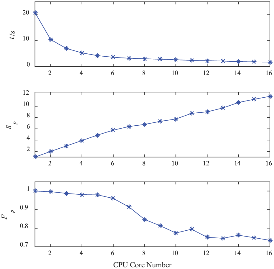
Computational time, speedup ratio, and parallel efficiency with different CPU core numbers.

Figure 14.

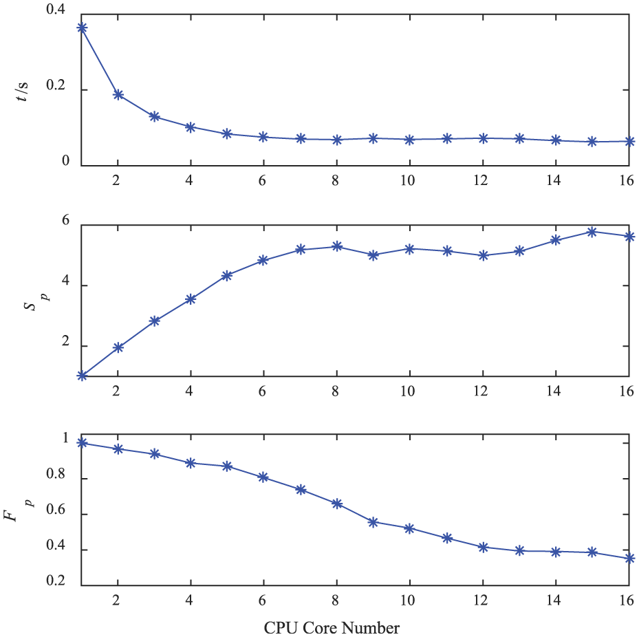
Computational time, speedup ratio, and parallel efficiency of the reduced computation scale.

Figure 15.

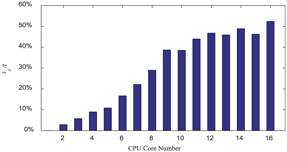
Proportion of average communication time t_c to computational time t.

Engineering example of an MLRS

An MSD model of MLRS with 18 launch tubes is shown in Figure 16. According to the natural properties of each MLRS components, these components can be regarded as dynamics elements including lumped masses, rigid bodies, elastic beams, springs, torsional springs, and so on and are sequentially numbered. The corresponding topology figure of the dynamics model is shown in Figure 17. The body elements labeled 2, 5, 8, 11, 14, and 17 are the wheels; 19 the vehicle body; 21 the revolving part; 23 the pitch part; 27 + 5l and 28 + 5l the segments of the launch tube; 26 + 5l the tail of the launch tube, where l stands for the launch tube in the firing state and $l=1,2,\dots ,18$ . The hinge elements are 24 + 5l and 25 + 5l connecting the launch tube to the pitch part; 22 connecting the revolving part to the pitch part; 20 connecting the vehicle body to the revolving part; 3, 6, 9, 12, 15, and 18 connecting the wheels to the vehicle body; 1, 4, 7, 10, 13, and 16 connecting the wheels to the ground. The system has eight boundary points in total, where ${\mathit{Z}}_{28+5l,0}$ and ${\mathit{Z}}_{26+5l,0}$ are the free ends at the front and tail of the launch tube, respectively; ${\mathit{Z}}_{1,0}$ , ${\mathit{Z}}_{4,0}$ , ${\mathit{Z}}_{7,0}$ , ${\mathit{Z}}_{10,0}$ , ${\mathit{Z}}_{13,0}$ , and ${\mathit{Z}}_{16,0}$ are the connection ends of hinges 1, 4, 7, 10, 13, and 16 connected to the ground. The boundary ${\mathit{Z}}_{28+5l,0}$ is considered as the root of the system, and all other boundaries ( ${\mathit{Z}}_{26+5l,0}$ , ${\mathit{Z}}_{1,0}$ , ${\mathit{Z}}_{4,0}$ , ${\mathit{Z}}_{7,0}$ , ${\mathit{Z}}_{10,0}$ , ${\mathit{Z}}_{13,0}$ , and ${\mathit{Z}}_{16,0}$ ) are considered as the treetop of the system. The transfer direction of the system is from the treetop to the root as the arrow direction shown in Figure 17.

Figure 16.

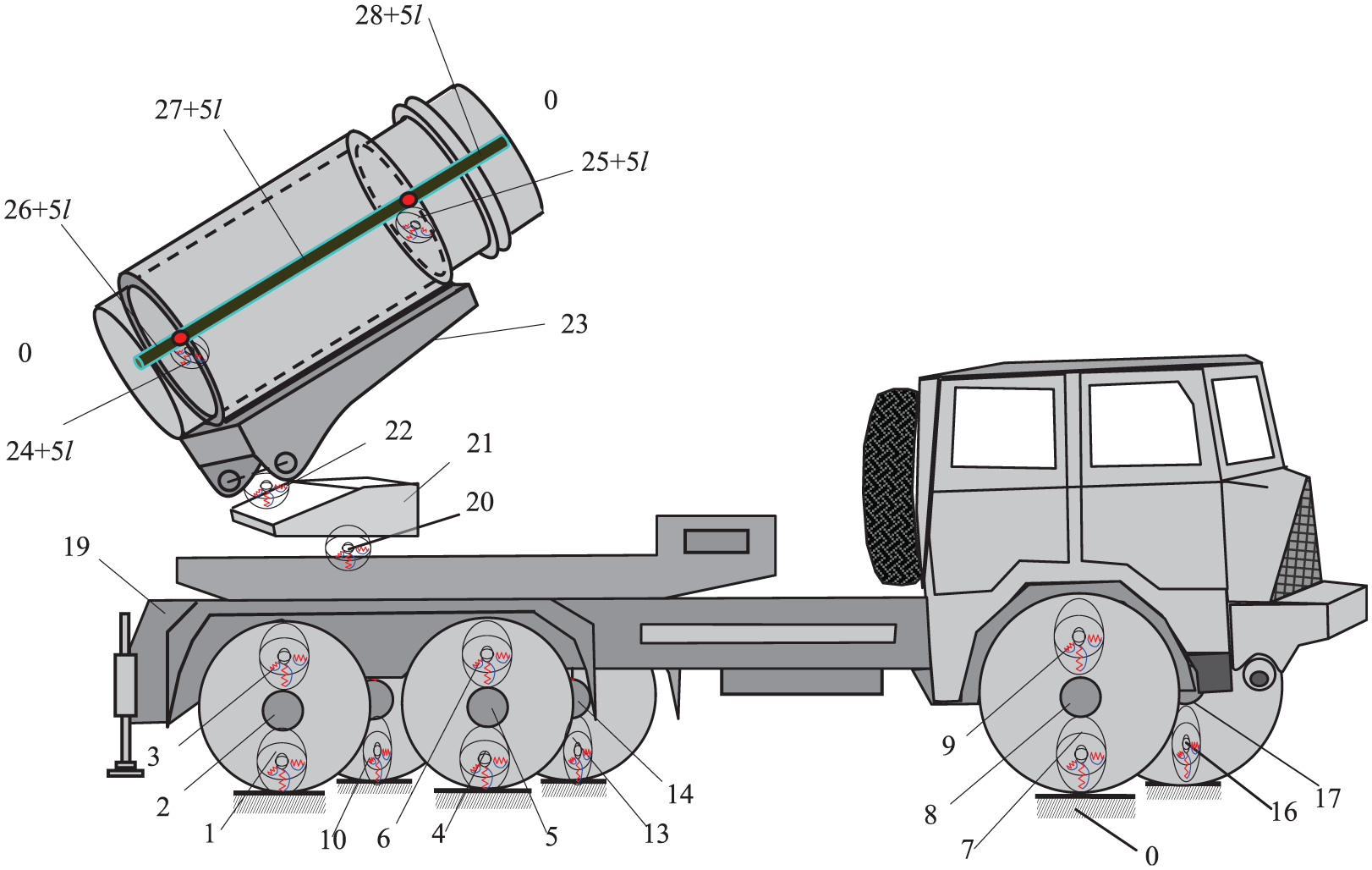
MSD model of MLRS.

Figure 17.

Topology figure of MSD model of MLRS.

Based on the topology of the MLRS dynamics model, the overall transfer equation and the overall transfer matrix of the MLRS given by equations (22)–(24) can be obtained by applying the automatic deduction theorem of the overall transfer equation of multibody systems ¹¹

$${\mathit{U}}_{\mathrm{all}}{\mathit{Z}}_{\mathrm{all}}=0$$

(22)

$$\begin{array}{cc}\multicolumn{1}{c}{{\mathit{Z}}_{\mathrm{all}}=}& [{\mathit{Z}}_{28+5l,0}^{\mathrm{T}},{\mathit{Z}}_{1,0}^{\mathrm{T}},{\mathit{Z}}_{4,0}^{\mathrm{T}},{\mathit{Z}}_{7,0}^{\mathrm{T}},{\mathit{Z}}_{10,0}^{\mathrm{T}},{\mathit{Z}}_{13,0}^{\mathrm{T}},\hfill \\ \multicolumn{1}{c}{}& {\mathit{Z}}_{16,0}^{\mathrm{T}},{\mathit{Z}}_{26+5l,0}^{\mathrm{T}},{\mathit{Z}}_{23,25+5l}^{\mathrm{T}}{]}^{\mathrm{T}}\hfill \end{array}$$

(23)

$${\mathit{U}}_{\mathrm{all}}=\left[\begin{array}{ccccccccc}\begin{array}{c}-{\mathit{I}}_{12}\hfill \\ \multicolumn{1}{c}{\mathit{O}}\\ \multicolumn{1}{c}{\mathit{O}}\\ \multicolumn{1}{c}{\mathit{O}}\\ \multicolumn{1}{c}{\mathit{O}}\\ \multicolumn{1}{c}{\mathit{O}}\\ \multicolumn{1}{c}{\mathit{O}}\\ \multicolumn{1}{c}{\mathit{O}}\\ \multicolumn{1}{c}{\mathit{O}}\end{array}\hfill & \begin{array}{c}{\mathit{T}}_{1-28+5l}\hfill \\ \multicolumn{1}{c}{{\mathit{G}}_{1-19}}\\ \multicolumn{1}{c}{{\mathit{G}}_{1-19}}\\ \multicolumn{1}{c}{{\mathit{G}}_{1-19}}\\ \multicolumn{1}{c}{{\mathit{G}}_{1-19}}\\ \multicolumn{1}{c}{{\mathit{G}}_{1-19}}\\ \multicolumn{1}{c}{{\mathit{G}}_{1-23}}\\ \multicolumn{1}{c}{{\mathit{G}}_{1-27+5l}}\\ \multicolumn{1}{c}{{\mathit{G}}_{1-28+5l}}\end{array}\hfill & \begin{array}{c}{\mathit{T}}_{4-28+5l}\hfill \\ \multicolumn{1}{c}{{\mathit{G}}_{4-19}}\\ \multicolumn{1}{c}{\mathit{O}}\\ \multicolumn{1}{c}{\mathit{O}}\\ \multicolumn{1}{c}{\mathit{O}}\\ \multicolumn{1}{c}{\mathit{O}}\\ \multicolumn{1}{c}{{\mathit{G}}_{4-23}}\\ \multicolumn{1}{c}{{\mathit{G}}_{4-27+5l}}\\ \multicolumn{1}{c}{{\mathit{G}}_{4-28+5l}}\end{array}\hfill & \begin{array}{c}{\mathit{T}}_{7-28+5l}\hfill \\ \multicolumn{1}{c}{\mathit{O}}\\ \multicolumn{1}{c}{{\mathit{G}}_{7-19}}\\ \multicolumn{1}{c}{\mathit{O}}\\ \multicolumn{1}{c}{\mathit{O}}\\ \multicolumn{1}{c}{\mathit{O}}\\ \multicolumn{1}{c}{{\mathit{G}}_{7-23}}\\ \multicolumn{1}{c}{{\mathit{G}}_{7-27+5l}}\\ \multicolumn{1}{c}{{\mathit{G}}_{7-28+5l}}\end{array}\hfill & \begin{array}{c}{\mathit{T}}_{10-28+5l}\hfill \\ \multicolumn{1}{c}{\mathit{O}}\\ \multicolumn{1}{c}{\mathit{O}}\\ \multicolumn{1}{c}{{\mathit{G}}_{10-19}}\\ \multicolumn{1}{c}{\mathit{O}}\\ \multicolumn{1}{c}{\mathit{O}}\\ \multicolumn{1}{c}{{\mathit{G}}_{10-23}}\\ \multicolumn{1}{c}{{\mathit{G}}_{10-27+5l}}\\ \multicolumn{1}{c}{{\mathit{G}}_{10-28+5l}}\end{array}\hfill & \begin{array}{c}{\mathit{T}}_{13-28+5l}\hfill \\ \multicolumn{1}{c}{\mathit{O}}\\ \multicolumn{1}{c}{\mathit{O}}\\ \multicolumn{1}{c}{\mathit{O}}\\ \multicolumn{1}{c}{{\mathit{G}}_{13-19}}\\ \multicolumn{1}{c}{\mathit{O}}\\ \multicolumn{1}{c}{{\mathit{G}}_{13-23}}\\ \multicolumn{1}{c}{{\mathit{G}}_{13-27+5l}}\\ \multicolumn{1}{c}{{\mathit{G}}_{13-28+5l}}\end{array}\hfill & \begin{array}{c}{\mathit{T}}_{16-28+5l}\hfill \\ \multicolumn{1}{c}{\mathit{O}}\\ \multicolumn{1}{c}{\mathit{O}}\\ \multicolumn{1}{c}{\mathit{O}}\\ \multicolumn{1}{c}{\mathit{O}}\\ \multicolumn{1}{c}{{\mathit{G}}_{16-19}}\\ \multicolumn{1}{c}{{\mathit{G}}_{16-23}}\\ \multicolumn{1}{c}{{\mathit{G}}_{16-27+5l}}\\ \multicolumn{1}{c}{{\mathit{G}}_{16-28+5l}}\end{array}\hfill & \begin{array}{c}{\mathit{T}}_{26+5l-28+5l}\hfill \\ \multicolumn{1}{c}{\mathit{O}}\\ \multicolumn{1}{c}{\mathit{O}}\\ \multicolumn{1}{c}{\mathit{O}}\\ \multicolumn{1}{c}{\mathit{O}}\\ \multicolumn{1}{c}{\mathit{O}}\\ \multicolumn{1}{c}{\mathit{O}}\\ \multicolumn{1}{c}{{\mathit{G}}_{26+5l-27+5l}}\\ \multicolumn{1}{c}{{\mathit{G}}_{26+5l-28+5l}}\end{array}\hfill & \begin{array}{c}{\mathit{T}}_{23-28+5l}\mathit{C}+{\mathit{T}}_{25+5l-28+5l}\hfill \\ \multicolumn{1}{c}{\mathit{O}}\\ \multicolumn{1}{c}{\mathit{O}}\\ \multicolumn{1}{c}{\mathit{O}}\\ \multicolumn{1}{c}{\mathit{O}}\\ \multicolumn{1}{c}{\mathit{O}}\\ \multicolumn{1}{c}{{\mathit{G}}_{23-23}\mathit{C}}\\ \multicolumn{1}{c}{{\mathit{G}}_{23-27+5l}\mathit{C}}\\ \multicolumn{1}{c}{{\mathit{G}}_{23-28+5l}\mathit{C}+{\mathit{G}}_{25+5l-28+5l}}\end{array}\hfill \end{array}\right]$$

(24)

where ${\mathit{Z}}_{23,25+5l}$ means the state vector of the connection point between body 23 and hinge 25 + 5l in the closed loop, ${\mathit{U}}_{\mathrm{all}}$ is the overall transfer matrix, ${\mathit{I}}_{12}$ is a 12 × 12 identity matrix, ${\mathit{T}}_{i-28+5l}(i=1,4,7,10,13,16,23,25+5l,26+5l)$ , and ${\mathit{G}}_{i-j}(i=1,4,7,10,13,16,23,25+5l,26+5l;j=19,23,27+5l,28+5l)$ are the coefficient matrices in the main transfer equation and geometry equations of the overall transfer equation of a system, respectively. ¹¹ The transfer matrix of each element could be found in Rui et al.^10,16

Eliminating all zeros in ${\mathit{Z}}_{\mathrm{all}}$ corresponding to the known variables in the system boundary conditions, and removing the columns associated with these zeros in ${\mathit{U}}_{\mathrm{all}}$ , equation (22) reduced to

$${\overline{\mathit{U}}}_{\mathrm{all}}{\overline{\mathit{Z}}}_{\mathrm{all}}=0$$

(25)

The characteristic equation can be obtained as

$$\det {\overline{\mathit{U}}}_{\mathrm{all}}=0$$

(26)

The eigenvalues of the MLRS can be solved by applying the proposed method in this article. Furthermore, the computational time, speedup ratio, and parallel efficiency of the fully loaded MLRS with its first 50 computed eigenvalues by applying the suggested method are shown in Table 8. Moreover, the corresponding curves with different CPU core numbers are shown in Figure 18. Similar to the non-uniform beam, the parallel computing technique substantially increases the computational speed of the eigenvalues of the MLRS.

Table 8.

Parallel computational time, speedup ratio, and parallel efficiency.

Scheme no.	Number of process	Computational time t (s)	Speedup ratio Sp	Parallel efficiency Fp
1	1 (Single PC)	4.2457	1.0000	1.0000
2	2 (Single PC)	2.1295	1.9938	0.9969
3	4 (Single PC)	1.0862	3.9089	0.9772
4	1 + 1 (Distributed)	2.1366	1.9872	0.9936
5	1 + 1 + 1 + 1 (Distributed)	1.0883	3.9012	0.9753
6	2 + 2 + 2 + 2 (Distributed)	0.6562	6.4701	0.8088
7	3 + 3 + 3 + 3 (Distributed)	0.6205	6.8426	0.5702
8	4 + 4 + 4 + 4 (Distributed)	0.5193	8.1755	0.5110

Figure 18.

Computational time, speedup ratio, and parallel efficiency with different CPU core numbers.

During the design period, optimization on the parameters of MLRS such as connecting stiffness among MLRS components is an important step of the dynamics design. The firing interval of the MLRS is 0.6 s, namely, the launching frequency is about 1.67 Hz. The natural frequency of MLRS should keep away from the launching frequency to avoid resonances. According to the existing empirical natural frequency of other MLRSs, taking the first 10 eigenvalues of the fully loaded MLRS as optimization objective, and taking the stiffness among components of MLRS as design variables, the genetic algorithm is applied to optimize the dynamics performance of the MLRS. The optimization flow chart is shown in Figure 19. Figure 20 shows the first 10 eigenvalues of the MLRS varying with the genetic generations during the optimization process. The estimation evolution of the best fitness is shown in Figure 21. The eigenvalues obtained by computation and modal test are shown in Table 9. It can be seen that the computational results are in good agreement with those obtained by the experiment.

Figure 19.

The optimization flow chart of MLRS.

Figure 20.

The eigenvalues of MLRS.

Figure 21.

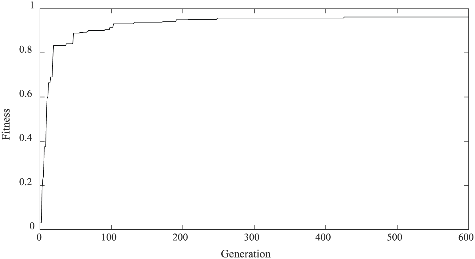
Convergence of the best fitness.

Table 9.

Comparison between the computational eigenvalues and the experimental values of MLRS.

Modal order (fully loaded)	Computational eigenvalues (Hz)	Experimental eigenvalues (Hz)	Relative error (%)
1	3.00	3.00	0.00
2	3.56	3.73	−4.56
3	5.17	5.23	−1.24
4	5.98	5.74	4.23
5	6.21	6.24	−0.53
6	7.19	6.73	6.83
7	8.77	8.71	0.64
8	9.79	10.60	−7.59
9	11.31	10.81	4.68
10	15.37	14.56	5.56

Table 10 shows the computational time by applying the proposed method and by a single process, respectively, which reveals the value of applying the proposed method to the dynamics optimization of complex multibody systems.

Table 10.

Comparison of computational time.

Number of process	Computational time t (h)
Single process	3.59
4 + 4 + 4 + 4 (Distributed)	0.44

Conclusion

The parallel algorithms for assembling the overall transfer matrix and recursive eigenvalue search are proposed based on MPI parallel computing theory in this article. The eigenvalues of a non-uniform beam and an MLRS are computed using this method. The influence of the CPU core number and the network environment on the computational time is analyzed. This study shows the following points:

1. The proposed parallel computing algorithm can significantly increase the computational speed to search eigenvalues and efficiently reduce the time cost of the dynamics optimization of complex multibody systems.

2. The distributed parallel computing environment based on MPI has strong scalability and high performance. It makes it possible to use ordinary computers to construct a computer cluster so that hardware resources can be fully utilized to achieve higher computational efficiency. Moreover, in order to achieve higher computational efficiency, good network environment is essential because the network environment has a certain impact on computational time.

3. With the increase in the number of CPU cores, the computational efficiency decreases due to the increase in the communication between processes. Therefore, computational time cannot be reduced infinitely by continually increasing the number of CPU cores. Appropriate number of CPU cores should be selected according to the computation scale.